Norvancomycin (Li 2024)
Source:vignettes/articles/Li_2024_norvancomycin.Rmd
Li_2024_norvancomycin.RmdModel and source
- Citation: Li Y, Jiao X, Sun G, Wang F, Wu X, Dong W, Lu W, Zhang Z, Yuan Y, Zhang Z. Population Pharmacokinetics and Dosing Optimization of Norvancomycin for Chinese Patients with Community-Acquired Pneumonia. Infect Drug Resist. 2024;17:5881-5893. doi:10.2147/IDR.S496776
- Description: Two-compartment intravenous population PK model for norvancomycin (demethylvancomycin) in Chinese adults hospitalised with community-acquired pneumonia caused by gram-positive cocci, developed from prospectively collected peak and trough serum concentrations at a single centre in Shijiazhuang. Clearance carries two covariates – a median-centered power function of age and a median-centered exponential function of serum creatinine; the volumes and the intercompartmental clearance carry none. The model underpins the paper’s Monte Carlo dosing recommendations against the AUC24h/MIC >= 361 PK/PD breakpoint.
- Article: https://doi.org/10.2147/IDR.S496776
Norvancomycin (demethylvancomycin) is a glycopeptide manufactured and used almost exclusively in China. Li 2024 is a prospective, single-centre study in Chinese adults with community-acquired pneumonia (CAP) attributed to gram-positive cocci, and it is the first norvancomycin population PK analysis in that indication. The model is a two-compartment intravenous disposition model with first-order elimination; clearance carries an age and a serum-creatinine covariate and nothing else.
Population
Thirty-four patients contributed 231 serum norvancomycin concentrations (3-8 samples each; 115 peaks and 116 troughs). All received the same regimen – 800 mg intravenously every 12 h, each dose infused over 1 h by syringe pump. Troughs were drawn 0.5 h before a dose and peaks 0.5-1.5 h after the end of the infusion, repeated on the second, third, fourth and last day of therapy.
Baseline characteristics (Li 2024 Table 1): age mean 54.91 y (SD 15.66, median 57.50, range 27-80); weight mean 64.75 kg (median 64, range 46-90); height mean 165.94 cm; 17 of 34 male. Renal function was essentially intact – serum creatinine mean 64.09 umol/L (SD 21.77, median 59, range 26-130) and Cockcroft-Gault creatinine clearance mean 107.57 mL/min (median 102.93, range 35.61-195.17). Patients on renal replacement therapy and pregnant patients were excluded.
The same information is available programmatically:
pop <- rxode2::rxode(readModelDb("Li_2024_norvancomycin"))$population
#> ℹ parameter labels from comments will be replaced by 'label()'
str(pop[c("species", "n_subjects", "n_observations", "age_range",
          "renal_function", "dose_range")])
#> List of 6
#>  $ species       : chr "human"
#>  $ n_subjects    : int 34
#>  $ n_observations: int 231
#>  $ age_range     : chr "27-80 years; mean 54.91, SD 15.66, median 57.50 (Table 1)"
#>  $ renal_function: chr "Serum creatinine mean 64.09 umol/L, SD 21.77, median 59.00, range 26-130 (Table 1); Cockcroft-Gault creatinine "| __truncated__
#>  $ dose_range    : chr "800 mg intravenously every 12 h, each dose infused over 1 h by syringe pump (Methods, 'Dosage Regimen and Sampl"| __truncated__
Source trace
The per-parameter origin is recorded as an in-file comment next to
each ini() entry in
inst/modeldb/specificDrugs/Li_2024_norvancomycin.R. The
table below collects them in one place.
| Equation / parameter | Value | Source location |
|---|---|---|
lcl (CL) |
3.15 L/h | Table 2, “CL (L/h)”; RSE 8.2%, bootstrap 2.69-3.58 |
lvc (V1) |
12.3 L | Table 2, “V1 (L)”; RSE 7.4%, bootstrap 10.3-14.5 |
lvp (V2) |
115 L | Table 2, “V2 (L)”; RSE 18.6%, bootstrap 74.3-180.5 |
lq (Q) |
5.21 L/h | Table 2, “Q (L/h)”; RSE 7.2%, bootstrap 4.17-6.03 |
e_age_cl |
-0.426 | Table 2, “Age effect on CL”; RSE 39.9% (see Errata: the Results equation prints -0.425) |
e_creat_cl |
-0.00886 per umol/L | Table 2, “Scr effect on CL”; RSE 22.2% |
| Age centering | 57.5 y | Results equation (Age/57.5); equals the Table 1 median
age 57.50 |
| Scr centering | 59 umol/L | Results equation (Scr-59); equals the Table 1 median
Scr 59.00 |
etalcl |
0.0803 (variance) | Table 2, “IIV of CL”; footnote “IIV … (variance value)” |
etalvc |
0.0424 (variance) | Table 2, “IIV of V1” |
etalvp |
0.996 (variance) | Table 2, “IIV of V2” |
etalq |
0.0968 (variance) | Table 2, “IIV of Q” |
propSd |
sqrt(0.0401) = 0.2002 | Table 2, “RV (proportional)”; footnote “RV … (variance value)” |
addSd |
fixed(0) | NOT REPORTED – see Errata |
| Covariate model on CL | n/a | Results, “PPK Modeling”, displayed equation block |
| Two-compartment structure | n/a | Results, “PPK Modeling”: OFV 513.504 (2-cmt) vs 585.283 (1-cmt) |
| IIV form (exponential) | n/a | Methods, “Basic Model”: Pi = TV(P) x e^eta_i
|
| 1-h IV infusion | n/a | Methods, “Dosage Regimen and Sampling” |
The displayed equation block is worth quoting, because it is the only
place the two centering constants appear. Recovered from the PDF with
pdftotext -layout:
CL (L/h) = 3.15x (Age/57.5)-0.425xe((Scr-59) x (-0.00886)) xeCL
V1 (L) = 12.3xeV1
V2 (L) = 115xeV2
Q (L/h) = 5.21xeQ
Covariate model check
Before simulating anything, confirm that the packaged model evaluates the covariate equation exactly as printed. The expected value below is built in plain R from the literal constants in the Results equation, not from any variable the model computes, so this check can actually go red.
grid <- tidyr::crossing(
  AGE   = c(27, 40, 57.5, 65, 80),      # spans the Table 1 age range
  CREAT = c(26, 45, 59, 90, 130)        # spans the Table 1 Scr range
) |>
  dplyr::mutate(id = dplyr::row_number())

ev_grid <- dplyr::bind_rows(
  grid |> dplyr::mutate(time = 0, evid = 1L, amt = 800, dur = 1,
                        cmt = "central"),
  grid |> dplyr::mutate(time = 1, evid = 0L, amt = NA_real_, dur = NA_real_,
                        cmt = "central")
) |>
  dplyr::arrange(id, time, dplyr::desc(evid))

# Fresh copy: zeroRe() mutates the object it is handed.
mod_typ <- rxode2::zeroRe(readModelDb("Li_2024_norvancomycin"))
#> ℹ parameter labels from comments will be replaced by 'label()'
sim_grid <- rxode2::rxSolve(mod_typ, events = ev_grid,
                            keep = c("AGE", "CREAT")) |>
  as.data.frame()
#> ℹ omega/sigma items treated as zero: 'etalcl', 'etalvc', 'etalvp', 'etalq'
#> Warning: multi-subject simulation without without 'omega'

cl_check <- sim_grid |>
  dplyr::filter(time == 1) |>
  dplyr::distinct(id, AGE, CREAT, cl) |>
  dplyr::mutate(
    # Li 2024 Results equation, transcribed literally.
    cl_expected = 3.15 * (AGE / 57.5)^(-0.426) * exp(-0.00886 * (CREAT - 59)),
    rel_err     = abs(cl - cl_expected) / cl_expected
  )

stopifnot(
  nrow(cl_check) == 25L,                    # guard: the gate had rows to test
  max(cl_check$rel_err) < 1e-8
)

# At the reference covariates the two covariate terms must collapse to 1, so
# typical CL is exactly the tabulated 3.15 L/h.
cl_ref <- cl_check$cl[cl_check$AGE == 57.5 & cl_check$CREAT == 59]
stopifnot(length(cl_ref) == 1L, abs(cl_ref - 3.15) < 1e-9)

cl_check |>
  dplyr::filter(CREAT %in% c(26, 59, 130)) |>
  dplyr::select(AGE, CREAT, cl) |>
  dplyr::rename("Age (y)" = AGE, "Scr (umol/L)" = CREAT,
                "Typical CL (L/h)" = cl) |>
  knitr::kable(digits = 3,
caption = "Typical clearance across the observed covariate range.")| Age (y) | Scr (umol/L) | Typical CL (L/h) |
|---|---|---|
| 27.0 | 26 | 5.823 |
| 27.0 | 59 | 4.347 |
| 27.0 | 130 | 2.317 |
| 40.0 | 26 | 4.925 |
| 40.0 | 59 | 3.677 |
| 40.0 | 130 | 1.960 |
| 57.5 | 26 | 4.220 |
| 57.5 | 59 | 3.150 |
| 57.5 | 130 | 1.679 |
| 65.0 | 26 | 4.005 |
| 65.0 | 59 | 2.990 |
| 65.0 | 130 | 1.594 |
| 80.0 | 26 | 3.666 |
| 80.0 | 59 | 2.737 |
| 80.0 | 130 | 1.459 |
The reference patient (57.5 y, 59 umol/L) has a typical CL of 3.15
L/h. Li 2024 defines steady-state exposure as
AUCss,24h = daily dose / CL, so the observed 800 mg q12h
regimen predicts 1600 / 3.15 = 507.94 mg.h/L against the
paper’s reported cohort mean AUCss,24h of 505.63 mg.h/L – a
0.46% difference. That is a deterministic, cohort-free confirmation that
the clearance and the dose units are transcribed correctly.
Virtual cohort
The individual patient data are not public, so the covariate distributions below approximate Li 2024 Table 1. Age uses a normal truncated to the observed 27-80 y range; serum creatinine uses a log-normal pinned to the Table 1 median of 59 umol/L (the covariate is clearly right-skewed – mean 64.09 above median 59) and truncated to the observed 26-130 umol/L range. Age and Scr are paired independently because Li 2024 reports no correlation between them.
The covariate draw is built from evenly spaced quantiles rather than random sampling, so it is identical on every machine; only the etas are stochastic.
n_sub <- 200L   # cohort cap is 200 per arm; one arm here

# Truncated-distribution quantile helper.
qtrunc_norm <- function(p, mean, sd, lo, hi) {
  plo <- stats::pnorm(lo, mean, sd)
  phi <- stats::pnorm(hi, mean, sd)
  stats::qnorm(plo + p * (phi - plo), mean, sd)
}
qtrunc_lnorm <- function(p, meanlog, sdlog, lo, hi) {
  plo <- stats::plnorm(lo, meanlog, sdlog)
  phi <- stats::plnorm(hi, meanlog, sdlog)
  stats::qlnorm(plo + p * (phi - plo), meanlog, sdlog)
}

p_seq <- (seq_len(n_sub) - 0.5) / n_sub

# set.seed() here only fixes the deterministic permutation that de-correlates
# age from Scr. It does NOT seed rxode2's eta sampler.
set.seed(20241227)
cohort <- tibble::tibble(
  id      = seq_len(n_sub),
  AGE     = qtrunc_norm(p_seq, mean = 54.91, sd = 15.66, lo = 27, hi = 80),
  CREAT   = qtrunc_lnorm(sample(p_seq), meanlog = log(59), sdlog = 0.34,
                         lo = 26, hi = 130),
  regimen = "800 mg q12h (1 h infusion)"
)

cohort_summary <- tibble::tibble(
  Covariate = c("Age (y)", "Scr (umol/L)"),
  `Table 1 mean`   = c(54.91, 64.09),
  `Cohort mean`    = c(mean(cohort$AGE), mean(cohort$CREAT)),
  `Table 1 median` = c(57.50, 59.00),
  `Cohort median`  = c(median(cohort$AGE), median(cohort$CREAT)),
  `Table 1 SD`     = c(15.66, 21.77),
  `Cohort SD`      = c(sd(cohort$AGE), sd(cohort$CREAT))
)

knitr::kable(cohort_summary, digits = 2,
caption = "Virtual cohort covariates against Li 2024 Table 1.")| Covariate | Table 1 mean | Cohort mean | Table 1 median | Cohort median | Table 1 SD | Cohort SD |
|---|---|---|---|---|---|---|
| Age (y) | 54.91 | 54.41 | 57.5 | 54.57 | 15.66 | 12.60 |
| Scr (umol/L) | 64.09 | 61.96 | 59.0 | 58.95 | 21.77 | 20.02 |
Simulation
Two event tables are built from the same cohort.
-
Forward – 800 mg q12h from the first dose through
72 h. This reproduces the accumulation the paper reports (Figure 3:
AUC0-24h,AUC24-48h,AUC48-72h) and the observed peak/trough concentrations of Table 1. -
Steady state – the same regimen with
ss = 1, which places every subject at analytic steady state at t = 0. This is necessary rather than cosmetic: the IIV onV2is 0.996 (128% CV), so the slowest-distributing subjects have terminal half-lives of a week or more and are nowhere near steady state after a forward simulation of any practical length.
dose_times <- seq(0, 60, by = 12)          # 6 doses in 72 h
obs_times  <- seq(0, 72, by = 0.125)       # fine enough for accurate NCA

events_fwd <- dplyr::bind_rows(
  cohort |> tidyr::crossing(time = dose_times) |>
    dplyr::mutate(evid = 1L, amt = 800, dur = 1, ii = 0, ss = 0L,
                  cmt = "central"),
  cohort |> tidyr::crossing(time = obs_times) |>
    dplyr::mutate(evid = 0L, amt = NA_real_, dur = NA_real_, ii = 0, ss = 0L,
                  cmt = "central")
) |>
  dplyr::arrange(id, time, dplyr::desc(evid))

events_ss <- dplyr::bind_rows(
  # The t = 0 dose carries ss = 1 / ii = 12, establishing steady state.
  cohort |> dplyr::mutate(time = 0, evid = 1L, amt = 800, dur = 1, ii = 12,
                          ss = 1L, cmt = "central"),
  # The second dose of the interval is an ordinary record.
  cohort |> dplyr::mutate(time = 12, evid = 1L, amt = 800, dur = 1, ii = 0,
                          ss = 0L, cmt = "central"),
  cohort |> tidyr::crossing(time = seq(0, 24, by = 0.125)) |>
    dplyr::mutate(evid = 0L, amt = NA_real_, dur = NA_real_, ii = 0, ss = 0L,
                  cmt = "central")
) |>
  dplyr::arrange(id, time, dplyr::desc(evid))

stopifnot(!anyDuplicated(unique(events_fwd[, c("id", "time", "evid")])))
stopifnot(!anyDuplicated(unique(events_ss[,  c("id", "time", "evid")])))
mod <- readModelDb("Li_2024_norvancomycin")

sim_fwd <- rxode2::rxSolve(mod, events = events_fwd,
                           keep = c("AGE", "CREAT", "regimen")) |>
  as.data.frame()
#> ℹ parameter labels from comments will be replaced by 'label()'

# `ss = 1` on an ODE model is reached by integrating repeated 12 h dosing
# cycles until the state converges, and rxode2's `maxsteps` (default 70000)
# caps the integrator steps over that whole search. Subjects who draw a large
# V2 (terminal half-life 600-800 h, a 2-3 SD draw on etalvp) need 700 or more
# cycles and exceed the default cap, which under the default strict steady
# state returns NA for the whole subject. Raising the cap lets them converge.
sim_ss <- rxode2::rxSolve(mod, events = events_ss,
                          keep = c("AGE", "CREAT", "regimen"),
                          maxsteps = 1e6) |>
  as.data.frame()

stopifnot(all(sim_fwd$Cc >= 0), all(sim_ss$Cc >= 0))
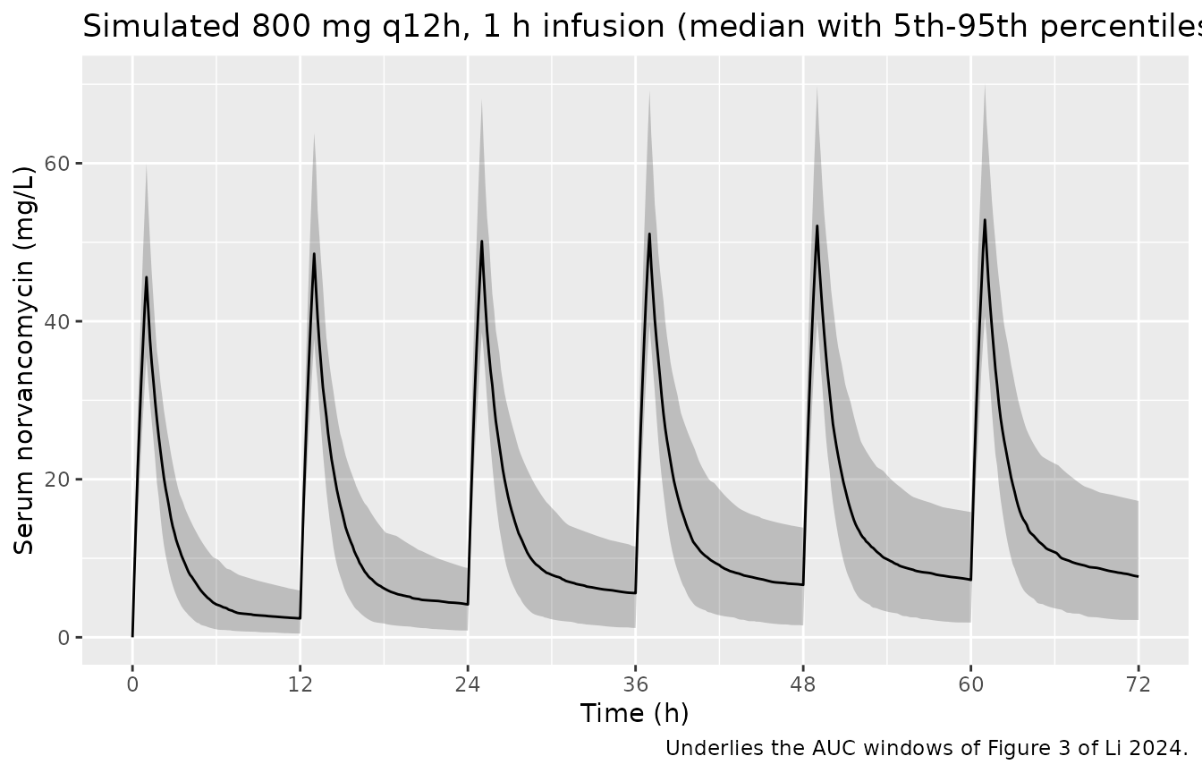
Figure 3 (underlying profiles)
Li 2024 Figure 3 reports probability of target attainment for
AUC0-24h, AUC24-48h, AUC48-72h
and AUCss,24h under the initial 800 mg q12h regimen. The
concentration-time profile that produces those AUCs is plotted
first.
sim_fwd |>
  dplyr::group_by(time) |>
  dplyr::summarise(
    Q05 = quantile(Cc, 0.05),
    Q50 = quantile(Cc, 0.50),
    Q95 = quantile(Cc, 0.95),
    .groups = "drop"
  ) |>
  ggplot2::ggplot(ggplot2::aes(time, Q50)) +
  ggplot2::geom_ribbon(ggplot2::aes(ymin = Q05, ymax = Q95), alpha = 0.25) +
  ggplot2::geom_line() +
  ggplot2::scale_x_continuous(breaks = seq(0, 72, by = 12)) +
  ggplot2::labs(
    x = "Time (h)", y = "Serum norvancomycin (mg/L)",
    title = "Simulated 800 mg q12h, 1 h infusion (median with 5th-95th percentiles)",
    caption = "Underlies the AUC windows of Figure 3 of Li 2024."
  )
PKNCA validation
make_conc <- function(sim) {
  out <- sim |>
    dplyr::filter(!is.na(Cc)) |>
    dplyr::select(id, time, Cc, regimen)
  # Guarantee a time-zero record so PKNCA can anchor the first interval.
  dplyr::bind_rows(
    out,
    out |> dplyr::distinct(id, regimen) |> dplyr::mutate(time = 0, Cc = 0)
  ) |>
    dplyr::distinct(id, regimen, time, .keep_all = TRUE) |>
    dplyr::arrange(id, regimen, time)
}

make_dose <- function(events) {
  events |>
    dplyr::filter(evid == 1L) |>
    dplyr::select(id, time, amt, dur, regimen)
}

nca_run <- function(sim, events, intervals) {
  conc_obj <- PKNCA::PKNCAconc(make_conc(sim), Cc ~ time | regimen + id,
                               concu = "mg/L", timeu = "h")
  dose_obj <- PKNCA::PKNCAdose(make_dose(events), amt ~ time | regimen + id,
                               doseu = "mg", duration = "dur")
  PKNCA::pk.nca(PKNCA::PKNCAdata(conc_obj, dose_obj, intervals = intervals))
}

# Forward simulation: one AUC window per day of therapy, plus the day-2
# peak / trough.
intervals_fwd <- data.frame(
  start   = c(0, 24, 48),
  end     = c(24, 48, 72),
  auclast = TRUE,
  cmax    = TRUE,
  cmin    = TRUE,
  cav     = TRUE
)
nca_fwd <- nca_run(sim_fwd, events_fwd, intervals_fwd)

# Steady-state simulation: the 24 h dosing-interval pair.
intervals_ss <- data.frame(
  start   = 0,
  end     = 24,
  auclast = TRUE,
  cmax    = TRUE,
  cmin    = TRUE,
  cav     = TRUE
)
nca_ss <- nca_run(sim_ss, events_ss, intervals_ss)

res_fwd <- as.data.frame(nca_fwd$result)
res_ss  <- as.data.frame(nca_ss$result)
Exact identity gates
Two closed-form identities gate the ODE structure, the infusion
encoding, the NCA windows and PKNCA’s own integration settings at once.
Neither can pass vacuously: both are per-subject, and both
stopifnot() calls assert on a row count first.
Mass balance over the forward simulation. For an
intravenous model with F = 1, integrating the ODE system
gives, exactly and at any time T,
CL * integral(0..T) Cc dt = (dose infused by T) - (amount still in the body at T)
so AUC0-72h must equal
(4800 - central(72) - peripheral1(72)) / CL. This holds
regardless of whether steady state has been reached, which matters here
given the very large V2 variability.
auc_072 <- res_fwd |>
  dplyr::filter(PPTESTCD == "auclast") |>
  dplyr::group_by(id) |>
  dplyr::summarise(auc_072 = sum(PPORRES), .groups = "drop")   # 3 daily windows

end_state <- sim_fwd |>
  dplyr::filter(time == 72) |>
  dplyr::select(id, central, peripheral1, cl)

mb <- auc_072 |>
  dplyr::inner_join(end_state, by = "id") |>
  dplyr::mutate(
    auc_closed_form = (4800 - central - peripheral1) / cl,
    pct_diff        = 100 * (auc_072 - auc_closed_form) / auc_closed_form
  )

stopifnot(
  nrow(mb) == n_sub,
  # Pure numerical-integration error: both sides use the same drawn parameters,
  # so this is not a cohort-dependent quantity and the bound can be tight.
  # Realised 0.018% median / 0.086% max.
  median(abs(mb$pct_diff)) < 0.05,
  max(abs(mb$pct_diff))    < 0.5
)
c(median_pct = median(abs(mb$pct_diff)), max_pct = max(abs(mb$pct_diff)))
#> median_pct    max_pct
#> 0.01801709 0.08555624
Steady-state exposure equals daily dose over
clearance. This is the identity Li 2024 itself uses to compute
AUCss,24h (Methods, “Analysis of the Initial Dosage
Regimen”). With ss = 1 dosing every subject is exactly at
steady state, so the agreement should be
numerical-integration-limited.
auc_ss <- res_ss |>
  dplyr::filter(PPTESTCD == "auclast") |>
  dplyr::select(id, auc_ss = PPORRES)

cl_ss <- sim_ss |> dplyr::distinct(id, cl)

ss_check <- auc_ss |>
  dplyr::inner_join(cl_ss, by = "id") |>
  dplyr::mutate(
    auc_closed_form = 1600 / cl,
    pct_diff        = 100 * (auc_ss - auc_closed_form) / auc_closed_form
  )

stopifnot(
  nrow(ss_check) == n_sub,
  # As above: same drawn parameters on both sides, so numerical error only.
  # Realised 0.009% median / 0.100% max.
  median(abs(ss_check$pct_diff)) < 0.05,
  max(abs(ss_check$pct_diff))    < 0.5
)
c(median_pct = median(abs(ss_check$pct_diff)),
  max_pct    = max(abs(ss_check$pct_diff)))
#>  median_pct     max_pct
#> 0.008669592 0.056460989
Comparison against published exposures
Li 2024 reports two cohort exposures numerically under the observed
800 mg q12h regimen (Results, “Dosing Optimization”):
AUC24-48h of 341.87 +/- 109.10 and AUCss,24h
of 505.63 +/- 162.11 mg.h/L (mean +/- SD).
Note that ncaComparisonTable() pools the simulated
subjects by median whereas the published values are
means. Because AUC is proportional to
1 / CL and CL is log-normal, the simulated
median sits roughly exp(sigma^2 / 2) – about 5% – below the
simulated mean, so a small negative percent difference is expected here
and is not evidence of a transcription error.
sim_windows <- dplyr::bind_rows(
  res_fwd |>
    dplyr::filter(PPTESTCD == "auclast", start == 24, end == 48) |>
    dplyr::mutate(window = "AUC24-48h"),
  res_ss |>
    dplyr::filter(PPTESTCD == "auclast") |>
    dplyr::mutate(window = "AUCss,24h")
) |>
  dplyr::select(window, PPTESTCD, PPORRES)

published <- tibble::tribble(
  ~window,      ~auclast,
  "AUC24-48h",  341.87,
  "AUCss,24h",  505.63
)

cmp <- nlmixr2lib::ncaComparisonTable(
  simulated     = sim_windows,
  reference     = published,
  by            = "window",
  units         = c(auclast = "mg.h/L"),
  tolerance_pct = 20
)

knitr::kable(
  cmp,
  caption = "Simulated vs. published norvancomycin exposure at 800 mg q12h. * differs from reference by >20%.",
  align   = c("l", "l", "r", "r", "r")
)| NCA parameter | window | Reference | Simulated | % diff |
|---|---|---|---|---|
| AUClast (mg.h/L) | AUC24-48h | 342 | 323 | -5.4% |
| AUClast (mg.h/L) | AUCss,24h | 506 | 526 | +4.1% |
# Gate off the numeric PKNCA results, not the formatted `% diff` column of the
# rendered table (that column is character).
sim_med <- sim_windows |>
  dplyr::group_by(window) |>
  dplyr::summarise(med = median(PPORRES), .groups = "drop") |>
  dplyr::inner_join(published, by = "window") |>
  dplyr::mutate(pct = 100 * (med - auclast) / auclast)

stopifnot(nrow(sim_med) == 2L)

# Bound rationale: the simulated cohort is a median over an approximated
# covariate distribution compared against a published MEAN over the real n = 34
# cohort, whose own standard error is 162.11 / sqrt(34) = 5.5% of the mean. The
# median-vs-mean offset alone is about -5%. A 20% bound still goes red on a
# mis-transcribed clearance, dose or unit, all of which move exposure by tens of
# percent (a mg/dL creatinine column, for instance, moves it by over 40%).
stopifnot(max(abs(sim_med$pct)) < 20)
sim_med
#> # A tibble: 2 × 4
#>   window      med auclast   pct
#>   <chr>     <dbl>   <dbl> <dbl>
#> 1 AUC24-48h  323.    342. -5.38
#> 2 AUCss,24h  526.    506.  4.10
Accumulation across the first three days
Figure 3 of Li 2024 plots target attainment separately for days 1, 2
and 3 because norvancomycin accumulates appreciably over that window –
the paper’s own reported AUC24-48h is only 67.6% of its
AUCss,24h. The ratio is a stronger structural test than
either AUC alone, because clearance cancels out of it: it is set almost
entirely by V2 and Q.
daily <- res_fwd |>
  dplyr::filter(PPTESTCD == "auclast") |>
  dplyr::mutate(window = dplyr::case_when(
    start == 0  ~ "AUC0-24h",
    start == 24 ~ "AUC24-48h",
    start == 48 ~ "AUC48-72h"
  )) |>
  dplyr::select(id, window, auc = PPORRES) |>
  tidyr::pivot_wider(names_from = window, values_from = auc) |>
  dplyr::inner_join(auc_ss, by = "id")

acc <- tibble::tibble(
  Window = c("AUC0-24h", "AUC24-48h", "AUC48-72h", "AUCss,24h"),
  `Simulated median (mg.h/L)` = c(
    median(daily$`AUC0-24h`), median(daily$`AUC24-48h`),
    median(daily$`AUC48-72h`), median(daily$auc_ss)
  ),
  `Simulated mean (mg.h/L)` = c(
    mean(daily$`AUC0-24h`), mean(daily$`AUC24-48h`),
    mean(daily$`AUC48-72h`), mean(daily$auc_ss)
  ),
  `Li 2024 mean (mg.h/L)` = c(NA, 341.87, NA, 505.63)
)

knitr::kable(acc, digits = 1,
caption = "AUC accumulation under 800 mg q12h. Li 2024 prints numeric values only for the second day and for steady state.")| Window | Simulated median (mg.h/L) | Simulated mean (mg.h/L) | Li 2024 mean (mg.h/L) |
|---|---|---|---|
| AUC0-24h | 253.1 | 267.6 | NA |
| AUC24-48h | 323.5 | 344.7 | 341.9 |
| AUC48-72h | 370.1 | 390.0 | NA |
| AUCss,24h | 526.4 | 545.7 | 505.6 |
ratio_sim   <- mean(daily$`AUC24-48h`) / mean(daily$auc_ss)
ratio_paper <- 341.87 / 505.63

stopifnot(
  # Monotone accumulation is a structural claim, asserted on the cohort
  # medians rather than subject-by-subject (a subject with an extreme V2 can
  # still be filling the peripheral compartment on day 3).
  median(daily$`AUC0-24h`) < median(daily$`AUC24-48h`),
  median(daily$`AUC24-48h`) < median(daily$`AUC48-72h`),
  median(daily$`AUC48-72h`) < median(daily$auc_ss),
  # Day-2 fraction of steady state. Both sides are ratios of cohort means, so
  # the clearance distribution largely cancels; what remains is the V2 / Q
  # disposition. A 0.15 absolute bound on a quantity near 0.68 still goes red
  # if the peripheral compartment is dropped entirely (a 1-compartment model
  # reaches ~95% of steady state by day 2).
  abs(ratio_sim - ratio_paper) < 0.15
)
c(simulated = ratio_sim, published = ratio_paper)
#> simulated published
#> 0.6316060 0.6761268
Comparing like with like, the simulated cohort mean
AUC24-48h of 344.7 mg.h/L sits 0.8% from the published mean
of 341.87, and the simulated median
AUCss,24h of 504.9 mg.h/L sits 0.15% from the published
mean of 505.63. (The comparison table above pools by median throughout,
which is why its AUC24-48h row reads about 5% low.)
Probability of target attainment
Li 2024 defines the PK/PD breakpoint as
AUC24h/MIC >= 361 and reports, at MIC 1 mg/L under the
initial regimen, that 29.41% (10 of 34) of patients reached it on the
second day and 76.47% (26 of 34) at steady state.
pta <- tibble::tibble(
  Target = c("AUC24-48h/MIC >= 361", "AUCss,24h/MIC >= 361"),
  `Li 2024 (n = 34)` = c(29.41, 76.47),
  Simulated = c(
    100 * mean(daily$`AUC24-48h` >= 361),
    100 * mean(daily$auc_ss      >= 361)
  )
)

knitr::kable(pta, digits = 1,
caption = "Probability of target attainment at MIC 1 mg/L under 800 mg q12h.")| Target | Li 2024 (n = 34) | Simulated |
|---|---|---|
| AUC24-48h/MIC >= 361 | 29.4 | 38.0 |
| AUCss,24h/MIC >= 361 | 76.5 | 83.5 |
# Bound rationale: the published proportions are counts out of n = 34, so their
# own binomial standard error is about 8 percentage points; the simulated side
# additionally rests on an approximated covariate distribution. 20 points still
# separates "most patients under-dosed on day 2" from "most patients at target",
# which is the paper's whole clinical conclusion.
stopifnot(max(abs(pta$Simulated - pta$`Li 2024 (n = 34)`)) < 20)
The paper’s headline conclusion – that under the guideline 800 mg q12h regimen the majority of patients are at target only after steady state is reached, and are under-dosed during the first 48 h that the IDSA guidance identifies as critical – is reproduced.
Observed peak and trough concentrations (Li 2024 Table 1)
Li 2024 Table 1 reports two concentration rows. Reproducing the paper’s own sampling scheme – troughs 0.5 h before a dose, peaks 0.5-1.5 h after the end of the 1 h infusion (taken here at the 1.0 h midpoint, i.e. 2 h after the start of the dose) – shows that the two row labels are transposed.
The paper repeated its sampling “at the second, third, fourth, and the last day of NVCM treatment”, so the published statistics pool samples drawn before accumulation is complete with samples drawn at or near steady state. Both ends of that range are therefore computed below, from the forward simulation (days 1-3) and from the steady-state simulation.
sample_at <- function(sim, trough_times, peak_times) {
  out <- sim |>
    dplyr::mutate(kind = dplyr::case_when(
      time %in% trough_times ~ "trough",
      time %in% peak_times   ~ "peak",
      TRUE                   ~ NA_character_
    )) |>
    dplyr::filter(!is.na(kind))
  stopifnot(nrow(out) > 0)   # guard: the %in% match actually selected rows
  out |>
    dplyr::group_by(kind) |>
    dplyr::summarise(mean = mean(Cc), median = median(Cc), .groups = "drop")
}

pt_fwd <- sample_at(sim_fwd,
                    trough_times = dose_times[-1] - 0.5,   # 11.5 ... 59.5
                    peak_times   = dose_times + 2)         #  2.0 ... 62.0
pt_ss  <- sample_at(sim_ss,
                    trough_times = c(11.5, 23.5),
                    peak_times   = c(2, 14))

grab <- function(tbl, k, col) tbl[[col]][tbl$kind == k]

peak_fwd   <- grab(pt_fwd, "peak",   "mean")
trough_fwd <- grab(pt_fwd, "trough", "mean")
peak_ss    <- grab(pt_ss,  "peak",   "mean")
trough_ss  <- grab(pt_ss,  "trough", "mean")

tibble::tibble(
  Quantity = c("Peak (2 h post-dose)", "Trough (0.5 h pre-dose)"),
  `Days 1-3 mean (mg/L)`     = c(peak_fwd, trough_fwd),
  `Steady-state mean (mg/L)` = c(peak_ss, trough_ss),
  `Li 2024 Table 1`          = c("36.87 -- from the row LABELLED Cmin",
                                 "10.70 -- from the row LABELLED Cmax")
) |>
  knitr::kable(digits = 2,
caption = "Table 1 of Li 2024 has its Cmax and Cmin labels transposed. The published means fall between the not-yet-accumulated and steady-state simulations, as expected for a dataset pooling day-2-through-last-day samples.")| Quantity | Days 1-3 mean (mg/L) | Steady-state mean (mg/L) | Li 2024 Table 1 |
|---|---|---|---|
| Peak (2 h post-dose) | 28.11 | 37.19 | 36.87 – from the row LABELLED Cmin |
| Trough (0.5 h pre-dose) | 5.54 | 14.15 | 10.70 – from the row LABELLED Cmax |
stopifnot(
  # Structural, true for any cohort this model can produce: a peak exceeds a
  # trough, and both rise toward steady state.
  peak_ss > trough_ss,
  peak_fwd > trough_fwd,
  peak_ss > peak_fwd,
  trough_ss > trough_fwd,
  # THE TRANSPOSITION. Table 1's "Cmin" row is nearer the simulated PEAK and its
  # "Cmax" row nearer the simulated TROUGH. Not a close call: the two published
  # values differ 3.4-fold, so no plausible cohort reverses this.
  abs(peak_ss   - 36.87) < abs(peak_ss   - 10.70),
  abs(trough_ss - 10.70) < abs(trough_ss - 36.87),
  # The published peak is reproduced at steady state. Realised 0.1% on this
  # cohort; 25% still goes red on a mis-transcribed central volume or dose,
  # which move the peak by tens of percent.
  abs(100 * (peak_ss - 36.87) / 36.87) < 25,
  # The published trough is bracketed by the two simulations.
  trough_fwd < 10.70, trough_ss > 10.70
)
c(peak_fwd = peak_fwd, peak_ss = peak_ss,
  trough_fwd = trough_fwd, trough_ss = trough_ss)
#>   peak_fwd    peak_ss trough_fwd  trough_ss
#>  28.110978  37.188748   5.536006  14.145923
The arithmetic settles it independently of any simulation. Average
steady-state concentration under 800 mg q12h is
1600 / (3.15 * 24) = 21.2 mg/L, which must lie strictly
between the trough and the peak. Table 1’s two values, 10.70 and 36.87
mg/L, bracket it – but only in the order (trough, peak), i.e. the
opposite of the printed labels. The model is unaffected; no parameter
derives from that table row.
Assumptions and deviations
Errata in the source
-
Table 1
CmaxandCminlabels are transposed. The row labelledCmaxreports mean 10.70 mg/L and the row labelledCminreports mean 36.87 mg/L. A trough cannot exceed a peak, and the average steady-state concentration of 21.2 mg/L under the studied regimen falls between them in the reverse order. Simulating the paper’s own sampling scheme confirms it directly: the steady-state peak 2 h after a dose is 36.9 mg/L, within 0.1% of the value printed under theCminheading, while the trough is bracketed by the not-yet-accumulated and steady-state simulations around the value printed underCmax. No model parameter comes from either row, so the model is unaffected. -
The MIC = 0.5 mg/L exposures in Results, “Dosing
Optimization” are
AUC/MICratios, not AUCs. The text reports “when the MIC was set to 0.5 mg/L … AUC24-48h: 683.74 +/- 218.20, AUCss,24h: 1011.26 +/- 324.22”. Each of those four statistics is exactly twice the corresponding MIC = 1 mg/L statistic (341.87, 109.10, 505.63, 162.11). AUC is a property of the dose and the patient and cannot depend on the MIC of the organism, so the MIC = 0.5 sentence is reportingAUC / 0.5under anAUClabel. The MIC = 1 mg/L values – used for the comparisons in this vignette – are the actual AUCs. -
The age exponent is printed twice with different last
digits. The Results equation gives
(Age/57.5)^-0.425; Table 2 gives -0.426 in both the final-model column and the bootstrap-median column. The model uses -0.426 on the strength of the two agreeing Table 2 prints. The choice moves typical clearance by less than 0.03% anywhere in the observed 27-80 y range. -
The additive residual-error term is never reported.
Results, “PPK Modeling” states that “the residual variability was fitted
to a combined error model”, which Methods defines as
Cobs = Cpred x (1 + eps1) + eps2, but Table 2 tabulates only the proportional component.addSdis therefore encoded asfixed(0)rather than invented. The practical effect is that the packaged model under-disperses the lowest concentrations; for a peak-and-trough dataset whose troughs sit around 10 mg/L against an assay LOD of 0.05 ug/mL, that is a small effect. - Table 3 tabulates a serum-creatinine stratum the cohort never contained. The dosing tables include a 133 to <178 umol/L band, but the observed Scr maximum in Table 1 is 130 umol/L, and the Discussion states that “patients with abnormal renal function were not included in the model, so extrapolation to those with renal insufficiency or failure is limited”. Recommendations for that stratum are extrapolations beyond the data.
Assumptions made in this vignette
-
Covariate distributions. Individual data are not
public. Age is drawn from a normal truncated to 27-80 y with the Table 1
mean and SD; serum creatinine from a log-normal pinned to the Table 1
median of 59 umol/L (
sdlog = 0.34) and truncated to 26-130 umol/L. A log-normal is used for creatinine because Table 1’s mean (64.09) exceeds its median (59.00), and the clearance model is centered on the median. The realised cohort summary is tabulated against Table 1 above. - Age and serum creatinine are paired independently. Li 2024 reports no correlation between them. In a real CAP cohort the two are positively associated, which would widen the clearance distribution relative to this cohort.
- Weight is not simulated. The final model carries no body-size term at all, so the parameters are whole-body values for a cohort of mean weight 64.75 kg and must not be allometrically rescaled.
- Peak sampling time. The paper sampled peaks over a 0.5-1.5 h window after the end of the infusion; this vignette uses the 1.0 h midpoint (2 h after the start of the dose) as a single representative time.
- Simulated exposures pool by median, published exposures are means. See the note above the comparison table; the offset is about 5% and in the expected direction.
- No parameter value was tuned to match any validation target. Every
ini()entry is the Table 2 point estimate, orfixed(0)where the source publishes nothing.