Ondansetron CNS distribution with tariquidar in rats (Chiang 2024)
Source:vignettes/articles/Chiang_2024_ondansetron.Rmd
Chiang_2024_ondansetron.RmdModel and source
- Citation: Chiang M, Back H, Lee JB, Oh S, Guo T, Girgis S, Park C, Haroutounian S, Kagan L. Pharmacokinetic Modeling of the Effect of Tariquidar on Ondansetron Disposition into the Central Nervous System. Pharm Res. 2024;41(7):1401-1411. doi:10.1007/s11095-024-03739-6.
- Description (male): Preclinical (rat, male). Semi-physiological five-compartment PK model of intravenous ondansetron in male Sprague-Dawley rats (Chiang 2024): central and peripheral systemic disposition compartments with first-order elimination from central, and brain, spinal cord and cerebrospinal-fluid (CSF) compartments exchanging bidirectionally with central and with each other, plus first-order P-glycoprotein (Pgp) efflux from brain and spinal cord back to central. Fitted jointly to mean profiles of wild-type rats (ondansetron alone), Pgp-knockout (Mdr1a -/-) rats (Pgp efflux set to zero) and wild-type rats pretreated with the Pgp inhibitor tariquidar (separate central volume, elimination rate constant and Pgp efflux rate). CAUTION: with the published Table III values the model reproduces the paper’s concentrations only for an input dose of about 0.7-0.8 mg/kg, 1/12 to 1/14 of the stated 10 mg/kg (see the vignette).
- Article: https://doi.org/10.1007/s11095-024-03739-6 (open access, PMC11263240)
- Upstream model and wild-type / knockout data: Chiang M et al. Pharm Res. 2020;37:205, https://doi.org/10.1007/s11095-020-02929-2
Chiang 2024 fitted one semi-physiological model to the mean ondansetron profiles of three groups of rats: wild-type rats given ondansetron alone (WT), P-gp knockout rats given ondansetron alone (KO; data from the 2020 study), and wild-type rats given tariquidar 30 min before ondansetron (OT; this study). Male and female rats were fitted separately with the same structure, so the package carries two models:
| Model | Table III column |
|---|---|
Chiang_2024_ondansetron_male_rat |
Male |
Chiang_2024_ondansetron_female_rat |
Female |
The group is selected with two covariates:
CONMED_TARIQUIDAR (1 = OT group) and
STRAIN_ABCB1A_KO (1 = Mdr1a(-/-) knockout). The paper
studied tariquidar only in wild-type rats, so the two indicators are
never both 1.
Population
Wild-type Sprague-Dawley rats (males 10-12 weeks, 300-350 g; females 12-14 weeks, 250-280 g) received ondansetron 10 mg/kg as an IV bolus, alone or 30 min after tariquidar 7.5 mg/kg IV (Methods, Animals and Experimental Design). Serial plasma samples were taken to 4 h, and groups of n = 4-6 rats were sacrificed at 0.16-2.5 h for terminal plasma, brain, spinal cord and cisterna-magna CSF. The WT and KO (Mdr1a(-/-), SD-Abcb1a tm1sage) data come from the 2020 study. The model was fitted to the mean profiles with the Ubiquity R package; there is no between-animal variability.
The same information is available programmatically:
str(rxode2::rxode(readModelDb("Chiang_2024_ondansetron_male_rat"))$population)
#> List of 9
#>  $ species       : chr "rat (Sprague-Dawley, wild type and Mdr1a(-/-) Pgp knockout)"
#>  $ sex_female_pct: num 0
#>  $ n_studies     : num 2
#>  $ age_range     : chr "10-12 weeks"
#>  $ weight_range  : chr "300-350 g"
#>  $ disease_state : chr "healthy"
#>  $ dose_range    : chr "ondansetron 10 mg/kg IV bolus (jugular cannula or tail vein), alone or 30 min after tariquidar 7.5 mg/kg IV"
#>  $ regions       : chr "United States (Rutgers University)"
#>  $ notes         : chr "Mean (naive-pooled) concentration profiles fitted with the Ubiquity R package. Data: OT-M (ondansetron + tariqu"| __truncated__
Model structure
Chiang 2024 Eqs. 1-5, with states A1 = central, A2 =
peripheral1, A3 = brain, A4 =
spinal_cord and A5 = csf:
Table III estimates one constant for k35 = k45
(k_cns_csf) and one for k53 = k54
(k_csf_cns). kPgp
(k_cns_central_pgp) is set to zero in knockout rats and
replaced by the separately estimated kPgp,TRQ in the OT
group, which also has its own V1,TRQ and
kel,TRQ. Concentrations are amount divided by volume:
plasma Cc = central / V1,
Cbrain = brain / Vbrain,
Cspinal_cord = spinal_cord / Vspinal,
Ccsf = csf / VCSF.
Source trace
Every value is from Chiang 2024 Table III. The in-file comments in
inst/modeldb/specificDrugs/Chiang_2024_ondansetron_<sex>_rat.R
give the same locations.
| Parameter (model name) | Table III symbol | Male | Female | Unit |
|---|---|---|---|---|
lvc |
V1 | 17.5 | 13.3 | mL |
lvc + e_conmed_tariquidar_vc
|
V1,TRQ | 12.7 | 11.3 | mL |
lkel |
kel | 3.60 | 5.06 | 1/h |
lkel + e_conmed_tariquidar_kel
|
kel,TRQ | 3.38 | 3.02 | 1/h |
lk12 / lk21
|
k12 / k21 | 2.14 / 2.62 | 4.37 / 2.32 | 1/h |
lk_central_brain / lk_brain_central
|
k13 / k31 | 17.6 / 39.6 | 13.0 / 25.2 | 1/h |
lk_central_spinal_cord /
lk_spinal_cord_central
|
k14 / k41 | 9.37 / 71.0 | 3.60 / 31.5 | 1/h |
lk_central_csf / lk_csf_central
|
k15 / k51 | 0.081 / 6.84 | 0.518 / 47.3 | 1/h |
lk_cns_csf |
k35 = k45 | 0.928 | 0.914 | 1/h |
lk_csf_cns |
k53 = k54 | 66.6 | 79.9 | 1/h |
lk_cns_central_pgp |
kPgp | 81.9 | 101 | 1/h |
lk_cns_central_pgp +
e_conmed_tariquidar_k_cns_central_pgp
|
kPgp,TRQ | 0.002 | 0.0001 | 1/h |
lv_brain (fixed) |
Vbrain | 1.8 | 1.8 | mL |
lv_spinal_cord (fixed) |
Vspinal | 0.6 | 0.6 | mL |
lvcsf (fixed) |
VCSF | 0.25 | 0.25 | mL |
propSd, propSd_<output>
|
var_P (sqrt) | sqrt(0.05) | sqrt(0.03) | fraction |
| ODEs | Eqs. 1-5 | |||
KO: k_cns_central_pgp * (1 - STRAIN_ABCB1A_KO)
|
Methods, ‘set to zero in KO rats’ |
The three e_conmed_tariquidar_* effects are log-ratios
of the printed OT value to the ondansetron-alone value (for example
log(12.7 / 17.5)), so the model returns the printed
OT-group estimates exactly. The residual model follows the upstream 2020
paper, which defines the Ubiquity variance as
VAR = sigma1 * Yhat^2; one var_P is shared by
all four matrices.
The dose scale of the published parameters
Elimination occurs only from the central compartment, so the model’s
plasma AUC is Dose / (kel * V1) whatever the dose. With the
OT-M Table III values that clearance is only
3.38 * 12.7 = 43 mL/h, against the 525 mL/h that Table I
reports from the noncompartmental analysis of the same data. At the
stated 10 mg/kg dose (about 3250 ug for a 325 g rat) the model therefore
predicts a plasma AUC of about 76 ug*h/mL, against the observed 6.13.
The tissue concentrations scale the same way, because the brain,
spinal-cord and CSF volumes are fixed anatomical values.
The fitted curves in Figures 2 and 3 do agree with the Table III
values for an input of about 0.7-0.8 mg/kg. That is the dose for which
Dose / (kel * V1) equals the Table I AUC, and it is 1/12 to
1/14 of the stated dose. Neither Chiang 2024 nor the upstream 2020
paper, which shows the same gap, states what dose the fitting software
received. The maintainers therefore carry Table III exactly as printed,
and this article simulates the published figures at this effective dose,
back-solved from Table I for each sex:
male <- readModelDb("Chiang_2024_ondansetron_male_rat")
female <- readModelDb("Chiang_2024_ondansetron_female_rat")

# Effective dose = Table I AUC x kel,TRQ x V1,TRQ (OT group, this study).
dose_eff <- c(
  male = 6.13 * 3.38 * 12.7, # ug
  female = 5.65 * 3.02 * 11.3 # ug
)
# Nominal dose = 10 mg/kg x mid-range body weight (Methods, Animals).
bw_kg <- c(male = 0.325, female = 0.265)
dose_nominal <- 10 * 1000 * bw_kg # ug

tibble(
  Sex = names(dose_eff),
  `Nominal dose (ug)` = dose_nominal,
  `Effective dose (ug)` = round(dose_eff, 1),
  `Effective dose (mg/kg)` = round(dose_eff / 1000 / bw_kg, 2),
  `Nominal / effective` = round(dose_nominal / dose_eff, 1)
) |>
knitr::kable(caption = "Nominal and effective (back-solved) ondansetron doses.")| Sex | Nominal dose (ug) | Effective dose (ug) | Effective dose (mg/kg) | Nominal / effective |
|---|---|---|---|---|
| male | 3250 | 263.1 | 0.81 | 12.4 |
| female | 2650 | 192.8 | 0.73 | 13.7 |
The model is linear, so every dose-independent quantity is unaffected by this choice: tissue:plasma partition coefficients, half-lives, curve shapes, and the relative effect of P-gp inhibition. The checks below rely on those quantities.
Simulation
There is no between-animal variability, so the published fits are typical-value predictions. Only the residual error is removed.
# One typical rat per group: WT (ondansetron alone), KO (Pgp knockout) and OT
# (tariquidar pretreatment). Observation rows sit on the `central` ODE state
# with dvid = 1; every row returns all four concentrations.
groups <- tibble(
  group = c("WT", "KO", "OT"),
  CONMED_TARIQUIDAR = c(0, 0, 1),
  STRAIN_ABCB1A_KO = c(0, 1, 0)
)

make_events <- function(dose, times) {
  obs_times <- sort(unique(c(0, times)))
  bind_rows(lapply(seq_len(nrow(groups)), function(i) {
    bind_rows(
      tibble(time = 0, amt = dose, evid = 1L, cmt = "central", dvid = NA_integer_),
      tibble(time = obs_times, amt = 0, evid = 0L, cmt = "central", dvid = 1L)
    ) |>
      mutate(
        id = i,
        group = groups$group[i],
        CONMED_TARIQUIDAR = groups$CONMED_TARIQUIDAR[i],
        STRAIN_ABCB1A_KO = groups$STRAIN_ABCB1A_KO[i]
      )
  }))
}

simulate_sex <- function(mod, dose, times, params = NULL) {
  ev <- make_events(dose, times)
  typical <- rxode2::zeroRe(mod, which = "sigma")
  # The model has no IIV by design (fit to mean profiles), so rxode2's
  # "multi-subject simulation without omega" warning is expected here.
  sim <- withCallingHandlers(
    if (is.null(params)) {
      rxode2::rxSolve(typical, ev, keep = "group", returnType = "data.frame")
    } else {
      rxode2::rxSolve(typical, ev, params = params, keep = "group", returnType = "data.frame")
    },
    warning = function(w) {
      if (grepl("without 'omega'", conditionMessage(w), fixed = TRUE)) invokeRestart("muffleWarning")
    }
  )
  sim |>
    dplyr::select(id, group, time, Cc, Cbrain, Cspinal_cord, Ccsf)
}

fine_grid <- seq(0, 3, by = 0.01)
sim_fig <- bind_rows(
  simulate_sex(male, dose_eff[["male"]], fine_grid) |> mutate(sex = "Male"),
  simulate_sex(female, dose_eff[["female"]], fine_grid) |> mutate(sex = "Female")
)
Replicate published figures
Figures 2 and 3 – fitted profiles in WT, KO and OT rats
matrix_labels <- c(
  Cc = "Plasma", Cbrain = "Brain",
  Cspinal_cord = "Spinal cord", Ccsf = "CSF"
)
sim_fig |>
  pivot_longer(c(Cc, Cbrain, Cspinal_cord, Ccsf), names_to = "matrix", values_to = "conc") |>
  filter(time > 0) |>
  mutate(
    matrix = factor(matrix_labels[matrix], levels = matrix_labels),
    group = factor(group, levels = c("WT", "KO", "OT")),
    sex = factor(sex, levels = c("Male", "Female"))
  ) |>
  ggplot(aes(time, conc, colour = group, linetype = group)) +
  geom_line(linewidth = 0.8) +
  facet_grid(matrix ~ sex) +
  scale_y_log10() +
  coord_cartesian(ylim = c(0.01, 100)) +
  scale_colour_manual(values = c(WT = "navy", KO = "dodgerblue", OT = "forestgreen")) +
  labs(
    x = "Time (h)", y = "Ondansetron concentration (ug/mL)",
    colour = NULL, linetype = NULL,
    caption = paste(
      "Replicates the fitted lines of Figures 2 (male) and 3 (female) of",
      "Chiang 2024, at the effective dose."
    )
  ) +
  theme_bw()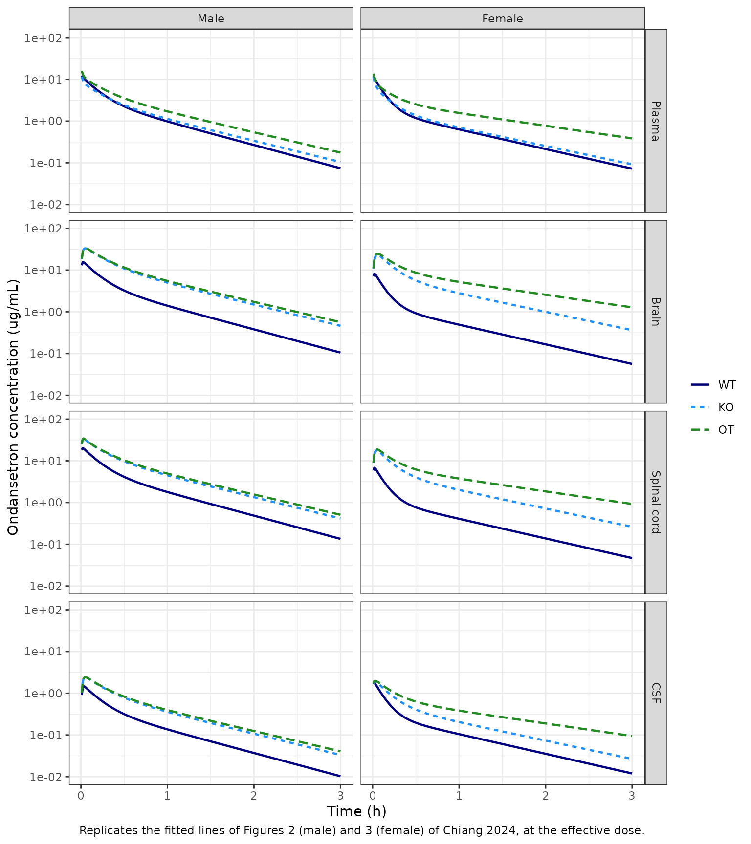
At the effective dose the plasma curves start near 15-20 ug/mL and fall by about two orders of magnitude by 3 h. The OT curves lie above WT and KO in every matrix, and in brain and spinal cord the KO curves lie well above WT. This is the pattern of the fitted lines in Figures 2 and 3. Simulated at the nominal dose, the curves have the same shape but sit 12-14 times higher.
Figures 6 and 7 – partial P-gp inhibition
The paper reduced the wild-type kPgp by 50% and 90%,
keeping either the WT systemic parameters (panels A, B) or the OT
systemic parameters (panels C, D). In the model this is an override of
lk_cns_central_pgp. For the OT panels the tariquidar effect
on kPgp is also switched off, so that kPgp is
the reduced wild-type value.
pgp_scenarios <- function(mod, dose, times) {
  ui <- rxode2::rxode(mod)
  lkpgp <- ui$iniDf$est[ui$iniDf$name == "lk_cns_central_pgp"]
  bind_rows(lapply(c(1, 0.5, 0.1), function(frac) {
    sim <- simulate_sex(
      mod, dose, times,
      params = c(
        lk_cns_central_pgp = lkpgp + log(frac),
        e_conmed_tariquidar_k_cns_central_pgp = 0
      )
    )
    sim |> mutate(pgp_reduction = paste0(round(100 * (1 - frac)), "%"))
  }))
}

sim_pgp <- bind_rows(
  pgp_scenarios(male, dose_eff[["male"]], fine_grid) |> mutate(sex = "Male"),
  pgp_scenarios(female, dose_eff[["female"]], fine_grid) |> mutate(sex = "Female")
)

# Reference curves: fitted WT, KO and OT, as drawn in Figures 6 and 7.
fitted_ref <- sim_fig |> mutate(pgp_reduction = paste("Fitted", group))
scen <- sim_pgp |>
  filter(pgp_reduction != "0%", group != "KO") |>
  mutate(
    panel = ifelse(group == "WT", "WT systemic", "OT systemic"),
    pgp_reduction = paste(pgp_reduction, "Pgp reduction")
  )
refs <- bind_rows(
  fitted_ref |> filter(group %in% c("WT", "KO")) |> mutate(panel = "WT systemic"),
  fitted_ref |> filter(group == "OT") |> mutate(panel = "OT systemic")
)
bind_rows(scen, refs) |>
  pivot_longer(c(Cbrain, Cspinal_cord), names_to = "matrix", values_to = "conc") |>
  filter(time > 0) |>
  mutate(
    matrix = matrix_labels[matrix],
    panel = factor(panel, levels = c("WT systemic", "OT systemic")),
    sex = factor(sex, levels = c("Male", "Female"))
  ) |>
  ggplot(aes(time, conc, colour = pgp_reduction)) +
  geom_line(linewidth = 0.7) +
  facet_grid(sex + panel ~ matrix) +
  scale_y_log10() +
  coord_cartesian(ylim = c(0.05, 100)) +
  labs(
    x = "Time (h)", y = "Ondansetron concentration (ug/mL)", colour = NULL,
    caption = "Replicates Figures 6 (male) and 7 (female) of Chiang 2024, at the effective dose."
  ) +
  theme_bw()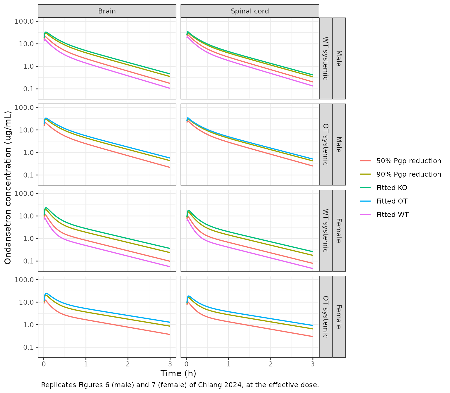
The Results text quantifies Figure 6 (WT systemic parameters, male): 1 h after the dose, a 50% and a 90% P-gp reduction raise the brain concentration 1.5- and 3-fold and the spinal-cord concentration 1.2- and 2-fold. These ratios do not depend on the dose.
fold_1h <- sim_pgp |>
  filter(group == "WT", abs(time - 1) < 1e-8) |>
  group_by(sex) |>
  mutate(
    brain_fold = Cbrain / Cbrain[pgp_reduction == "0%"],
    spinal_fold = Cspinal_cord / Cspinal_cord[pgp_reduction == "0%"]
  ) |>
  ungroup() |>
  filter(pgp_reduction != "0%") |>
  select(sex, pgp_reduction, brain_fold, spinal_fold)

published_fold <- tibble(
  sex = "Male", pgp_reduction = c("50%", "90%"),
  brain_pub = c(1.5, 3), spinal_pub = c(1.2, 2)
)
fold_cmp <- left_join(fold_1h, published_fold, by = c("sex", "pgp_reduction"))
fold_cmp |>
  mutate(across(c(brain_fold, spinal_fold), \(x) round(x, 2))) |>
  rename(
    "Sex" = sex, "Pgp reduction" = pgp_reduction,
    "Brain fold (model)" = brain_fold, "Brain fold (paper)" = brain_pub,
    "Spinal cord fold (model)" = spinal_fold, "Spinal cord fold (paper)" = spinal_pub
  ) |>
knitr::kable(caption = "Fold increase at 1 h over the fitted WT profile (WT systemic parameters).")| Sex | Pgp reduction | Brain fold (model) | Spinal cord fold (model) | Brain fold (paper) | Spinal cord fold (paper) |
|---|---|---|---|---|---|
| Male | 50% | 1.58 | 1.43 | 1.5 | 1.2 |
| Male | 90% | 2.87 | 2.19 | 3.0 | 2.0 |
| Female | 50% | 1.70 | 1.66 | NA | NA |
| Female | 90% | 3.88 | 3.53 | NA | NA |
male_fold <- filter(fold_cmp, sex == "Male")
# Deterministic typical-value solve: the brain folds sit within 6% of the
# quoted 1.5 and 3. The spinal-cord folds are discussed below.
stopifnot(all(abs(male_fold$brain_fold / male_fold$brain_pub - 1) < 0.10))
The brain folds agree with the text. The spinal-cord folds come out at about 1.4 and 2.2, a little above the quoted 1.2 and 2. They are, however, consistent with the curves drawn in Figure 6B, where the 50% curve at 1 h lies well above the fitted WT curve.
PKNCA validation
Plasma (Table I)
Table I comes from a noncompartmental analysis of the observed OT plasma profiles (sampling at 5, 10, 15, 30 and 45 min and 1, 1.5, 2, 2.5, 3 and 4 h), with the clearance and volume computed from the nominal 10 mg/kg dose. The simulated OT profiles are sampled on that schedule and reach PKNCA with the nominal dose. This reproduces the paper’s own calculation: the model concentrations at the effective dose stand in for the observed data.
plasma_times <- c(5, 10, 15, 30, 45) / 60
plasma_times <- c(plasma_times, 1, 1.5, 2, 2.5, 3, 4)
tissue_times <- c(0.16, 0.25, 0.5, 1, 1.5, 2, 2.5)

sim_nca <- bind_rows(
  simulate_sex(male, dose_eff[["male"]], sort(unique(c(plasma_times, tissue_times)))) |>
    mutate(sex = "Male"),
  simulate_sex(female, dose_eff[["female"]], sort(unique(c(plasma_times, tissue_times)))) |>
    mutate(sex = "Female")
) |>
  mutate(treatment = paste0(group, "-", substr(sex, 1, 1)))

plasma_nca_input <- sim_nca |>
  filter(!is.na(Cc), time == 0 | time %in% plasma_times) |>
  select(id, treatment, sex, time, Cc)
dose_nominal_df <- plasma_nca_input |>
  distinct(id, treatment, sex) |>
  mutate(time = 0, amt = dose_nominal[tolower(sex)])

conc_obj <- PKNCA::PKNCAconc(plasma_nca_input, Cc ~ time | treatment + id)
dose_obj <- PKNCA::PKNCAdose(dose_nominal_df, amt ~ time | treatment + id, route = "intravascular")
intervals <- data.frame(
  start = 0, end = Inf,
  aucinf.obs = TRUE, half.life = TRUE, mrt.iv.obs = TRUE,
  vss.iv.obs = TRUE, cl.obs = TRUE
)
nca_plasma <- PKNCA::pk.nca(PKNCA::PKNCAdata(conc_obj, dose_obj, intervals = intervals))

published_plasma <- tibble::tribble(
  ~treatment, ~half.life, ~aucinf.obs, ~mrt.iv.obs, ~vss.iv.obs, ~cl.obs,
  "OT-M", 0.638, 6.13, 0.577, 302, 525,
  "OT-F", 0.998, 5.65, 0.919, 396, 447
)
cmp_plasma <- nlmixr2lib::ncaComparisonTable(
  simulated = as.data.frame(nca_plasma) |> filter(treatment %in% published_plasma$treatment),
  reference = published_plasma,
  by = "treatment",
  units = c(
    half.life = "h", aucinf.obs = "h*ug/mL", mrt.iv.obs = "h",
    vss.iv.obs = "mL", cl.obs = "mL/h"
  ),
  tolerance_pct = 20
)
knitr::kable(
  cmp_plasma,
  caption = "Simulated (effective dose, nominal dose for NCA) vs. Table I. * differs by >20%."
)| NCA parameter | treatment | Reference | Simulated | % diff |
|---|---|---|---|---|
| AUC0-∞ (obs) (h*ug/mL) | OT-M | 6.13 | 6.34 | +3.4% |
| AUC0-∞ (obs) (h*ug/mL) | OT-F | 5.65 | 5.8 | +2.6% |
| t½ (h) | OT-M | 0.638 | 0.615 | -3.6% |
| t½ (h) | OT-F | 0.998 | 0.994 | -0.4% |
| CL/F (mL/h) | OT-M | 525 | 513 | -2.4% |
| CL/F (mL/h) | OT-F | 447 | 457 | +2.3% |
| MRT (IV) (h) | OT-M | 0.577 | 0.689 | +19.3% |
| MRT (IV) (h) | OT-F | 0.919 | 1.14 | +24.0%* |
| Vss (IV) (mL) | OT-M | 302 | 353 | +16.9% |
| Vss (IV) (mL) | OT-F | 396 | 521 | +31.6%* |
nca_plasma_wide <- as.data.frame(nca_plasma) |>
  filter(treatment %in% published_plasma$treatment) |>
  select(treatment, PPTESTCD, PPORRES) |>
  pivot_wider(names_from = PPTESTCD, values_from = PPORRES) |>
  left_join(published_plasma, by = "treatment", suffix = c("", "_pub"))
# Deterministic solve on the paper's sampling schedule. The half-life is dose-
# independent and matches Table I within 5% in both sexes. AUC, CL and Vss
# depend on the effective dose (back-solved from the Table I AUC), so they are
# compared at 20%: the residual difference is the trapezoid on the sparse
# schedule against the model's exact AUC.
stopifnot(
  all(abs(nca_plasma_wide$half.life / nca_plasma_wide$half.life_pub - 1) < 0.10),
  all(abs(nca_plasma_wide$aucinf.obs / nca_plasma_wide$aucinf.obs_pub - 1) < 0.20),
  all(abs(nca_plasma_wide$cl.obs / nca_plasma_wide$cl.obs_pub - 1) < 0.20)
)
The terminal half-life does not depend on the dose scale, and it agrees with Table I in both sexes. AUC and CL agree because the effective dose was back-solved from the Table I AUC. The model’s mean residence time is 19-24% longer than the Table I value, so Vss (= MRT x CL) comes out 17-32% larger. MRT does not depend on the dose either, so this is a property of the fitted parameters. The likeliest cause is that the observed 4-h profile resolves the model’s slow CNS-return phase less well than the model does.
Brain, spinal cord and CSF (Table II)
The tissue concentrations peak within minutes of the dose, before the first terminal sacrifice at 0.16 h. A trapezoid on the paper’s terminal schedule therefore underestimates the model’s tissue AUC by up to about 25%, from missing that peak alone. The model’s own tissue AUCs and partition coefficients are computed with PKNCA on a dense grid (every 0.02 h to 8 h), from the same solve for plasma and tissue.
dense_grid <- seq(0, 8, by = 0.02)
sim_dense <- bind_rows(
  simulate_sex(male, dose_eff[["male"]], dense_grid) |> mutate(sex = "Male"),
  simulate_sex(female, dose_eff[["female"]], dense_grid) |> mutate(sex = "Female")
) |>
  mutate(treatment = paste0(group, "-", substr(sex, 1, 1)))

dense_long <- sim_dense |>
  rename(Cplasma = Cc) |>
  pivot_longer(c(Cplasma, Cbrain, Cspinal_cord, Ccsf), names_to = "matrix", values_to = "Cc") |>
  filter(!is.na(Cc)) |>
  mutate(matrix = unname(c(
    Cplasma = "Plasma", Cbrain = "Brain", Cspinal_cord = "Spinal cord", Ccsf = "CSF"
  )[matrix])) |>
  select(id, treatment, sex, matrix, time, Cc)
dose_dense <- dense_long |>
  distinct(id, treatment, sex, matrix) |>
  mutate(time = 0, amt = dose_eff[tolower(sex)])

nca_tissue <- PKNCA::pk.nca(PKNCA::PKNCAdata(
  PKNCA::PKNCAconc(dense_long, Cc ~ time | treatment + matrix + id),
  PKNCA::PKNCAdose(dose_dense, amt ~ time | treatment + matrix + id),
  intervals = data.frame(start = 0, end = Inf, aucinf.obs = TRUE, half.life = TRUE)
))

published_tissue <- tibble::tribble(
  ~treatment, ~matrix, ~half.life, ~aucinf.obs,
  "OT-M", "Brain", 0.580, 22.0,
  "OT-F", "Brain", 0.352, 19.16,
  "OT-M", "Spinal cord", 0.907, 15.0,
  "OT-F", "Spinal cord", 0.596, 15.6,
  "OT-M", "CSF", 0.517, 1.37,
  "OT-F", "CSF", 0.580, 1.49
)
cmp_tissue <- nlmixr2lib::ncaComparisonTable(
  simulated = as.data.frame(nca_tissue) |>
    filter(treatment %in% c("OT-M", "OT-F"), matrix != "Plasma"),
  reference = published_tissue,
  by = c("treatment", "matrix"),
  units = c(half.life = "h", aucinf.obs = "h*ug/mL"),
  tolerance_pct = 20
)
knitr::kable(cmp_tissue, caption = "Simulated (effective dose) vs. Table II. * differs by >20%.")| NCA parameter | treatment | matrix | Reference | Simulated | % diff |
|---|---|---|---|---|---|
| AUC0-∞ (obs) (h*ug/mL) | OT-M | Brain | 22 | 19 | -13.6% |
| AUC0-∞ (obs) (h*ug/mL) | OT-M | Spinal cord | 15 | 17.3 | +15.3% |
| AUC0-∞ (obs) (h*ug/mL) | OT-M | CSF | 1.37 | 1.36 | -0.4% |
| AUC0-∞ (obs) (h*ug/mL) | OT-F | Brain | 19.2 | 18.2 | -5.1% |
| AUC0-∞ (obs) (h*ug/mL) | OT-F | Spinal cord | 15.6 | 13.2 | -15.6% |
| AUC0-∞ (obs) (h*ug/mL) | OT-F | CSF | 1.49 | 1.35 | -9.6% |
| t½ (h) | OT-M | Brain | 0.58 | 0.616 | +6.3% |
| t½ (h) | OT-M | Spinal cord | 0.907 | 0.616 | -32.0%* |
| t½ (h) | OT-M | CSF | 0.517 | 0.616 | +19.2% |
| t½ (h) | OT-F | Brain | 0.352 | 0.994 | +182.4%* |
| t½ (h) | OT-F | Spinal cord | 0.596 | 0.994 | +66.8%* |
| t½ (h) | OT-F | CSF | 0.58 | 0.994 | +71.4%* |
The OT-group tissue AUCs are within about 20% of Table II. The tissue half-lives in Table II are more scattered, because they come from terminal samples of 4-6 rats per time point. They run from 0.35 to 0.91 h, whereas the model gives every compartment the same terminal half-life as plasma (0.62 h in males, 1.0 h in females). In females, the model’s tissue half-lives are well above the Table II values.
Partition coefficients (Table II)
The partition coefficient is AUCtissue / AUCplasma. It does not
depend on the dose. Table II reports KP_OT from this study
and copies KP_WT and KP_KO from the 2020
study.
auc_dense <- as.data.frame(nca_tissue) |>
  filter(PPTESTCD == "aucinf.obs") |>
  select(treatment, matrix, auc = PPORRES)
kp <- auc_dense |>
  filter(matrix != "Plasma") |>
  left_join(
    auc_dense |> filter(matrix == "Plasma") |> select(treatment, auc_plasma = auc),
    by = "treatment"
  ) |>
  mutate(kp_model = auc / auc_plasma)

published_kp <- tibble::tribble(
  ~treatment, ~Brain, ~`Spinal cord`, ~CSF,
  "OT-M", 3.58, 2.44, 0.223, "OT-F", 3.39, 2.76, 0.263,
  "WT-M", 0.46, 0.39, 0.06, "WT-F", 0.71, 0.47, 0.11,
  "KO-M", 2.52, 1.78, 0.19, "KO-F", 3.04, 1.34, 0.22
) |>
  pivot_longer(-treatment, names_to = "matrix", values_to = "kp_paper")

kp_cmp <- left_join(kp, published_kp, by = c("treatment", "matrix")) |>
  mutate(pct_diff = 100 * (kp_model / kp_paper - 1))
kp_cmp |>
  mutate(across(c(kp_model, pct_diff), \(x) signif(x, 3))) |>
  arrange(matrix, treatment) |>
  select(matrix, treatment, kp_model, kp_paper, pct_diff) |>
  rename(
    "Matrix" = matrix, "Group" = treatment, "Kp (model)" = kp_model,
    "Kp (Table II)" = kp_paper, "Difference (%)" = pct_diff
  ) |>
knitr::kable(caption = "Model partition coefficients vs. Table II.")| Matrix | Group | Kp (model) | Kp (Table II) | Difference (%) |
|---|---|---|---|---|
| Brain | KO-F | 3.770 | 3.040 | 24.100 |
| Brain | KO-M | 4.260 | 2.520 | 69.100 |
| Brain | OT-F | 3.210 | 3.390 | -5.180 |
| Brain | OT-M | 3.090 | 3.580 | -13.600 |
| Brain | WT-F | 0.753 | 0.710 | 6.080 |
| Brain | WT-M | 1.390 | 0.460 | 201.000 |
| CSF | KO-F | 0.278 | 0.220 | 26.600 |
| CSF | KO-M | 0.306 | 0.190 | 61.000 |
| CSF | OT-F | 0.238 | 0.263 | -9.460 |
| CSF | OT-M | 0.222 | 0.223 | -0.411 |
| CSF | WT-F | 0.160 | 0.110 | 45.500 |
| CSF | WT-M | 0.135 | 0.060 | 125.000 |
| Spinal cord | KO-F | 2.730 | 1.340 | 104.000 |
| Spinal cord | KO-M | 3.880 | 1.780 | 118.000 |
| Spinal cord | OT-F | 2.330 | 2.760 | -15.600 |
| Spinal cord | OT-M | 2.820 | 2.440 | 15.400 |
| Spinal cord | WT-F | 0.625 | 0.470 | 33.000 |
| Spinal cord | WT-M | 1.770 | 0.390 | 354.000 |
kp_ot <- filter(kp_cmp, treatment %in% c("OT-M", "OT-F"))
# Deterministic; the OT-group Kp lie within about 16% of Table II in all six
# cells (brain -13 / -5%, spinal cord +16 / -15%, CSF 0 / -9%, male / female).
stopifnot(all(abs(kp_ot$pct_diff) < 20))
For the OT groups the model reproduces KP_OT within 16%
in every matrix. For the WT and KO groups the model partition
coefficients are well above the 2020 values in Table II: 3-fold above in
WT male brain and 4.5-fold above in WT male spinal cord. WT female brain
is the exception and agrees within 6%. These rows compare the 2024 joint
refit with the 2020 noncompartmental analysis, not with a model
prediction. The ratio of the fitted brain and plasma curves at 1 h in
Figure 2 (about 1.3 for WT-M, about 5 for KO-M) agrees with the model
(1.4 and 4.4), so the difference lies in the published refit and is not
an extraction error. It is listed below as a known deviation.
Exposure at the nominal dose
For completeness, the model simulated at the stated 10 mg/kg dose:
nominal <- bind_rows(
  simulate_sex(male, dose_nominal[["male"]], c(1, 2)) |> mutate(sex = "Male"),
  simulate_sex(female, dose_nominal[["female"]], c(1, 2)) |> mutate(sex = "Female")
) |>
  filter(group == "OT", time == 1)
nominal_auc <- c(
  male = dose_nominal[["male"]] / (3.38 * 12.7),
  female = dose_nominal[["female"]] / (3.02 * 11.3)
)
tibble(
  Sex = c("Male", "Female"),
  `Model plasma AUC at 10 mg/kg (h*ug/mL)` = round(nominal_auc, 1),
  `Table I AUC (h*ug/mL)` = c(6.13, 5.65),
  `Model plasma C at 1 h (ug/mL)` = round(nominal$Cc, 1)
) |>
knitr::kable(caption = "OT group at the nominal dose: the model is 12-14 times above the data.")| Sex | Model plasma AUC at 10 mg/kg (h*ug/mL) | Table I AUC (h*ug/mL) | Model plasma C at 1 h (ug/mL) |
|---|---|---|---|
| Male | 75.7 | 6.13 | 21.1 |
| Female | 77.7 | 5.65 | 21.5 |
Assumptions and deviations
- Dose scale. The Table III parameters reproduce the paper’s concentrations only for an input of about 0.7-0.8 mg/kg, 1/12 to 1/14 of the stated 10 mg/kg (see “The dose scale of the published parameters”). The upstream 2020 model shows the same gap. The maintainers carry Table III exactly as printed, without rescaling any parameter. The figures in this article use an effective dose back-solved from the Table I AUC: 263 ug in males and 193 ug in females. To predict the absolute concentrations after a known physical dose, scale that dose by the same factor. Dose-independent quantities (partition coefficients, half-lives, fold changes from P-gp inhibition) can be used directly.
- Body weights for the nominal dose are the mid-points of the Methods ranges (325 g male, 265 g female). The Table I CL and AUC imply 322 g and 253 g.
-
Shared rate constants. Table III reports single
values for
k35 = k45andk53 = k54, and a singlekPgpacting on both brain and spinal cord. These are encoded ask_cns_csf,k_csf_cnsandk_cns_central_pgp, so CSF loses2 * k_csf_cns * csf(Eq. 5). -
Tariquidar is a time-fixed categorical covariate,
as in the paper; its long half-life left no information for a
concentration-driven inhibition model.
CONMED_TARIQUIDAR = 1withSTRAIN_ABCB1A_KO = 1was not studied. -
Residual error.
var_Pis taken as the proportional variancesigma1of the 2020 paper (VAR = sigma1 * Yhat^2), shared by all four matrices. The model has no between-animal variability because it was fitted to mean profiles. - Known deviations. Against the 2020 noncompartmental values in Table II, the WT and KO partition coefficients are up to 4.5-fold higher (all but WT female brain more than 20% higher). The spinal-cord fold changes at 1 h (about 1.4 and 2.2) are above the 1.2 and 2 quoted in the Results. In females the tissue half-lives are well above the Table II terminal-sample values. All three are properties of the published fit and are not tuned.
- No erratum or correction notice for Chiang 2024 was found (checked 2026-11-10).