Colistin (Plachouras 2009)
Source:vignettes/articles/Plachouras_2009_colistin.Rmd
Plachouras_2009_colistin.RmdModel and source
- Citation: Plachouras D, Karvanen M, Friberg LE, et al. Population pharmacokinetic analysis of colistin methanesulfonate and colistin after intravenous administration in critically ill patients with infections caused by gram-negative bacteria. Antimicrob Agents Chemother. 2009;53(8):3430-3436.
- Article: https://doi.org/10.1128/AAC.01361-08
- Description: Joint parent-metabolite popPK model. Colistin
methanesulfonate (CMS, the inactive prodrug) is administered
intravenously and hydrolysed in vivo to colistin (the active polymyxin).
CMS disposition is described by a 2-compartment model with linear
elimination; colistin by a 1-compartment model formed by a first-order
process from CMS. Because the fraction (
fm) of CMS that converts to colistin cannot be identified from these data alone, the colistin clearance and volume are reported and packaged as the apparent valuesCL/fmandV/fm.
Population
Eighteen critically ill adult patients (12 male, 6 female) with documented or probable infections caused by multidrug-resistant Gram-negative bacteria (mostly Acinetobacter baumannii, Pseudomonas aeruginosa, and Enterobacteriaceae) admitted to the Critical Care Unit or 4th Department of Internal Medicine at Attikon University General Hospital in Athens, Greece. Patients receiving continuous venovenous hemodiafiltration were excluded. Mean age 63.6 years (range 40-83); mean Cockcroft-Gault creatinine clearance 82.3 +/- 24.35 mL/min on day 1 (range 41-126); APACHE II median 13 (range 5-20); baseline characteristics tabulated in Plachouras 2009 Table 1.
The standard regimen was CMS 3 MU (~240 mg) every 8 h as a 15-min IV infusion. Two patients with creatinine clearance below 50 mL/min received the empirically reduced regimen of approximately 2 MU q8h (~160 mg q8h).
The same information is available programmatically via the model’s
population metadata
(readModelDb("Plachouras_2009_colistin")$population).
Source trace
The per-parameter origin is recorded as an in-file comment next to
each ini() entry in
inst/modeldb/specificDrugs/Plachouras_2009_colistin.R. The
table below collects the principal entries in one place for review.
| Quantity | Value | Source location |
|---|---|---|
| CMS CL | 13.7 L/h | Table 2, CMS, CL (liters/h) typical value |
| CMS V1 | 13.5 L | Table 2, CMS, V1 (liters) typical value |
| CMS Q | 133 L/h | Table 2, CMS, Q (liters/h) typical value |
| CMS V2 | 28.9 L | Table 2, CMS, V2 (liters) typical value |
| CMS proportional residual | 22.0 % | Table 2, CMS, Residual error, Proportional (%) |
| CMS additive residual | 9.11 nmol/L | Table 2, CMS, Residual error, Additive (nmol/liter) |
| IIV CMS CL | 37 % CV | Table 2, CMS, IIV (% CV) |
| Apparent colistin CL/fm | 9.09 L/h | Table 2, Colistin, CL/fm (liters/h) typical value |
| Apparent colistin V/fm | 189 L | Table 2, Colistin, V/fm (liters) typical value |
| Colistin proportional residual | 7.19 % | Table 2, Colistin, Residual error, Proportional (%) |
| Colistin additive residual | 4.98 nmol/L | Table 2, Colistin, Residual error, Additive (nmol/liters) |
| IIV apparent colistin CL/fm | 59 % CV | Table 2, Colistin, IIV (% CV) |
| CMS molar mass | 1743 g/mol | Methods - Population pharmacokinetic modeling, p. 3431 |
| Colistin molar mass | 1163 g/mol | Methods - Population pharmacokinetic modeling, p. 3431 |
| CMS structural model (2-cmt) | n/a | Results - Data analysis, p. 3431 |
| Colistin structural model (1-cmt) | n/a | Results - Data analysis, p. 3431 |
| Half-life CMS fast phase | 0.046 h | Results, p. 3433 |
| Half-life CMS slow phase | 2.3 h | Results, p. 3433 |
| Half-life colistin | 14.4 h | Discussion, p. 3434 |
| Predicted Cmax first dose | 0.60 mg/L | Discussion, p. 3434 and Fig. 4 |
| Predicted Cmax steady state | 2.3 mg/L | Discussion, p. 3434 and Fig. 4 |
| Predicted Tmax first dose | ~7 h after infusion start | Discussion, p. 3434 |
Virtual cohort
The original observed concentration-time data are not publicly available. The figures below use a virtual population whose dosing covers the trial’s standard regimen (3 MU q8h ~ 240 mg CMS q8h as 15-min IV infusion). The Plachouras 2009 final model retained no covariate effects (Results - Data analysis), so demographics do not affect the typical-value predictions.
set.seed(20260601)

n_subjects     <- 50L         # virtual cohort for stochastic VPC
dose_mg        <- 240         # CMS dose per infusion (= 3 MU)
inf_dur_h      <- 15 / 60     # 15-min IV infusion
inf_rate       <- dose_mg / inf_dur_h
tau            <- 8           # h between doses
n_doses        <- 24          # > 14 half-lives of colistin (full SS)
sim_hours      <- n_doses * tau + 24
dose_times     <- seq(0, by = tau, length.out = n_doses)

build_subject_events <- function(id) {
  doses <- data.frame(
    id   = id,
    time = dose_times,
    amt  = dose_mg,
    cmt  = "central",
    evid = 1L,
    rate = inf_rate
  )
  # Observation grid: a single observation cmt per row (rxode2 emits BOTH
  # Cc and Cc_col on every row regardless of cmt label).
  obs <- data.frame(
    id   = id,
    time = seq(0.01, sim_hours, by = 0.25),
    amt  = NA_real_,
    cmt  = "Cc",
    evid = 0L,
    rate = NA_real_
  )
  ev <- dplyr::bind_rows(doses, obs)
  ev[order(ev$id, ev$time, ev$evid), ]
}

cohort <- lapply(seq_len(n_subjects), build_subject_events) |>
  dplyr::bind_rows()

stopifnot(!anyDuplicated(unique(cohort[, c("id", "time", "evid")])))
Simulation
mod <- rxode2::rxode(readModelDb("Plachouras_2009_colistin"))

# Stochastic cohort: full IIV included for the VPC-style trajectory plot.
sim <- rxode2::rxSolve(mod, events = cohort) |>
  as.data.frame()
For the typical-value trajectories used to reproduce Figure 4 and to compute NCA endpoints we also produce a single-subject prediction with the random effects zeroed out:
mod_typical  <- mod |> rxode2::zeroRe()
sim_typical  <- rxode2::rxSolve(mod_typical, events = cohort[cohort$id == 1L, ]) |>
  as.data.frame()
#> ℹ omega/sigma items treated as zero: 'etalcl', 'etalcl_col'
Replicate published trajectories
Plachouras 2009 Figure 4 displays the model-predicted CMS (panel A) and colistin (panel B) concentrations in a typical patient under the current dosing regimen (3 MU CMS q8h as 15-min infusion) and several alternative regimens with loading doses. The figure spans the first ~80 h of treatment, by which point the colistin profile has reached its steady-state plateau.
sim_typical |>
  dplyr::filter(time > 0, time <= 80) |>
  ggplot(aes(time, Cc)) +
  geom_line(linewidth = 0.8) +
  labs(x = "Time after first CMS dose (h)",
       y = "CMS plasma concentration (mg/L)",
       title = "Replicates Figure 4A of Plachouras 2009",
       caption = "Typical-value 3 MU CMS q8h regimen (15-min IV infusion).") +
  scale_y_log10()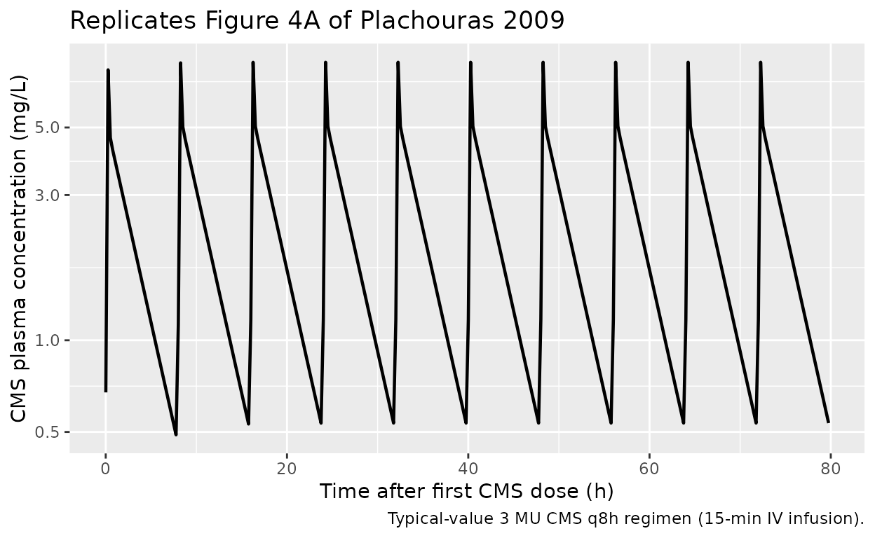
sim_typical |>
  dplyr::filter(time > 0, time <= 80) |>
  ggplot(aes(time, Cc_col)) +
  geom_line(linewidth = 0.8) +
  geom_hline(yintercept = 2, linetype = "dashed", colour = "grey40") +
  annotate("text", x = 5, y = 2.2, label = "MIC breakpoint (P. aeruginosa, A. baumannii)",
           hjust = 0, size = 3, colour = "grey30") +
  labs(x = "Time after first CMS dose (h)",
       y = "Colistin plasma concentration (mg/L)",
       title = "Replicates Figure 4B of Plachouras 2009",
       caption = "Typical-value 3 MU CMS q8h regimen. The dashed line marks the CLSI / EUCAST 2 mg/L susceptibility breakpoint.")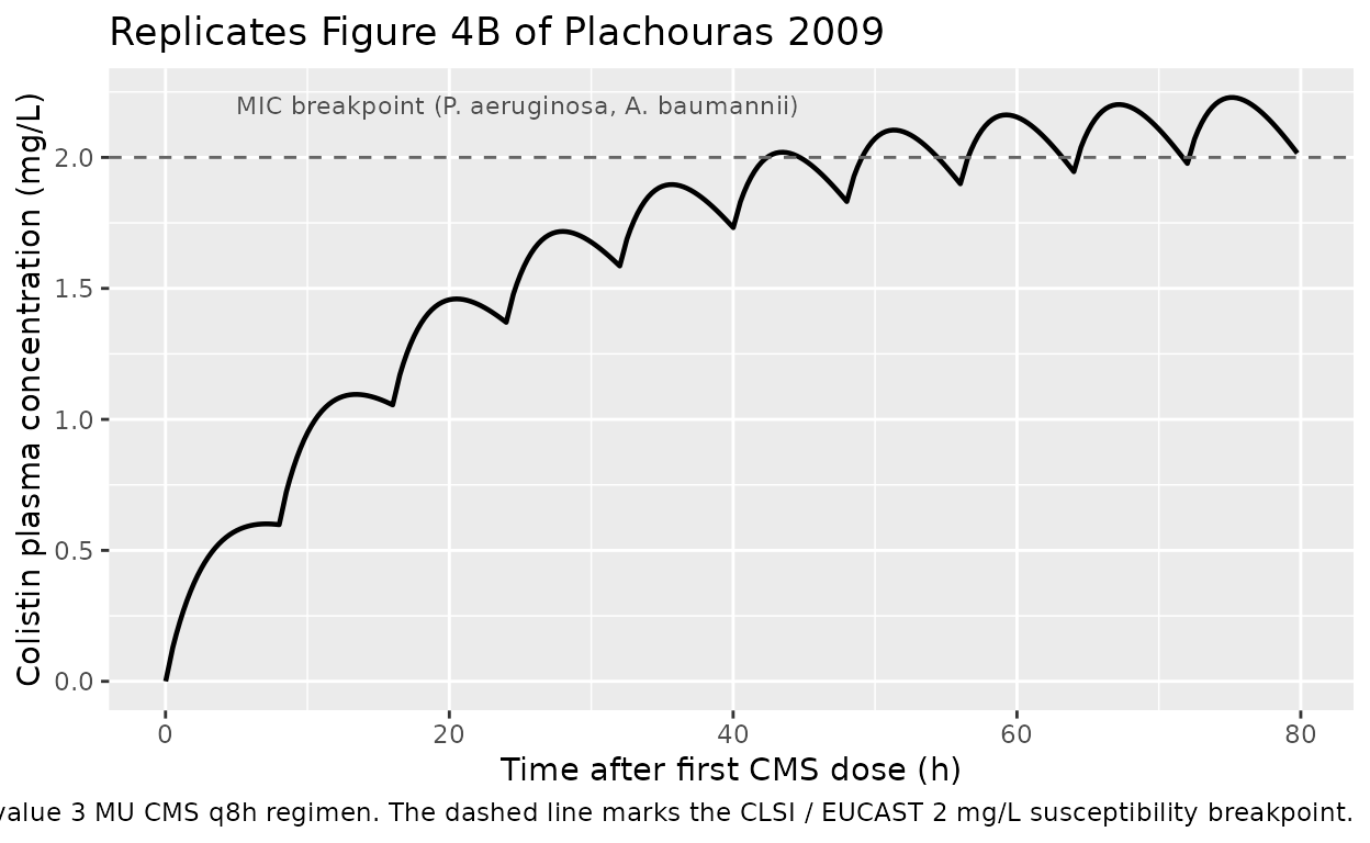
A stochastic VPC-style plot illustrates the between-subject variability driven by the IIV on CMS CL and apparent colistin CL/fm:
sim |>
  dplyr::filter(time > 0, time <= 80) |>
  dplyr::group_by(time) |>
  dplyr::summarise(
    Q05 = quantile(Cc_col, 0.05, na.rm = TRUE),
    Q50 = quantile(Cc_col, 0.50, na.rm = TRUE),
    Q95 = quantile(Cc_col, 0.95, na.rm = TRUE),
    .groups = "drop"
  ) |>
  ggplot(aes(time, Q50)) +
  geom_ribbon(aes(ymin = Q05, ymax = Q95), alpha = 0.25) +
  geom_line(linewidth = 0.8) +
  labs(x = "Time after first CMS dose (h)",
       y = "Colistin plasma concentration (mg/L)",
       title = "Stochastic colistin trajectory (50-subject virtual cohort)",
       caption = "Median and 5th-95th percentile envelope. IIV on CMS CL and apparent colistin CL/fm only (Plachouras 2009 Table 2).")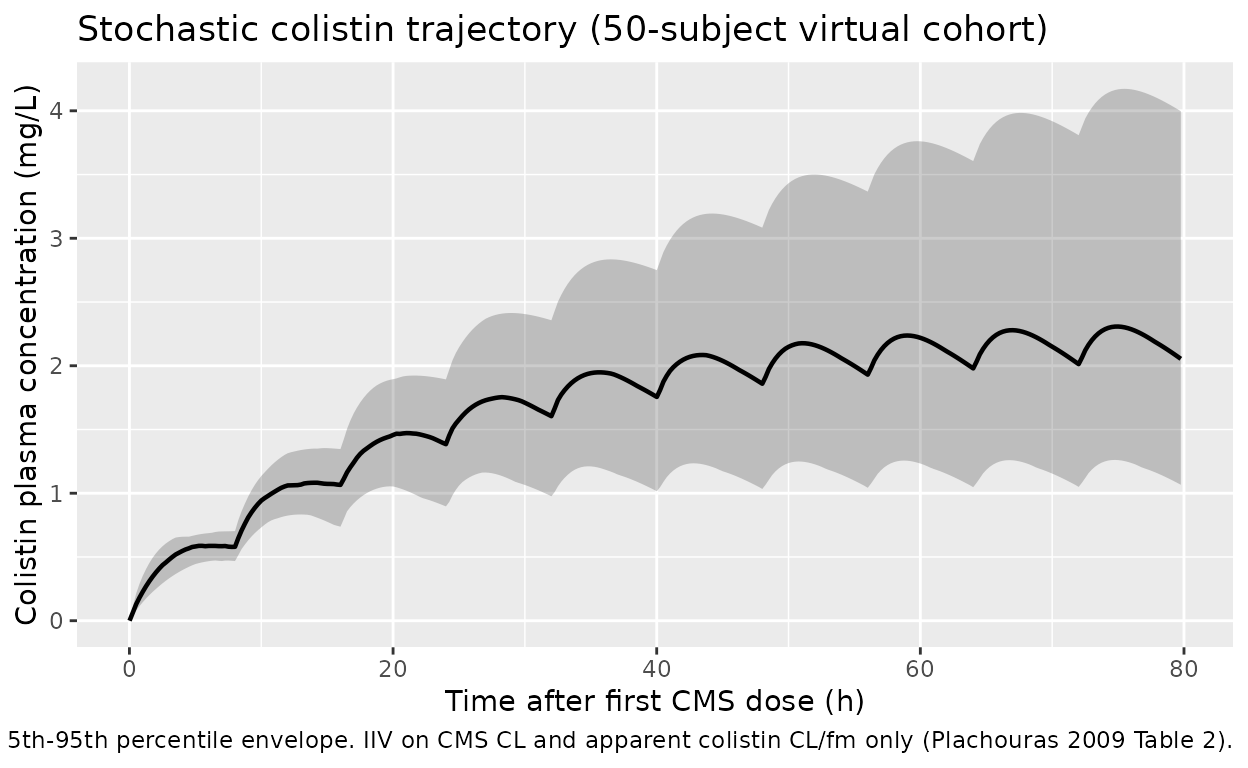
PKNCA validation
We compute Cmax and Tmax on the first-dose interval and on the
steady-state interval (the last interval in the 24-dose regimen) for
both analytes. The PKNCA formulas include a treatment label
so the per-interval summaries roll up cleanly even though we run a
single regimen.
# rxode2::rxSolve drops the `id` column when there is only one subject in the
# event table; restore it so the PKNCA `~ time | treatment + id` formulas
# below have a valid grouping column.
sim_typ <- sim_typical |>
  dplyr::mutate(id = 1L,
                treatment = "3 MU CMS q8h")

# First-dose interval ---------------------------------------------------------
sim_first <- sim_typ |>
  dplyr::filter(time >= 0, time <= tau)

dose_first <- data.frame(
  id        = 1L,
  time      = 0,
  amt       = dose_mg,
  treatment = "3 MU CMS q8h"
)
conc_cms_first <- PKNCA::PKNCAconc(
  sim_first |> dplyr::filter(!is.na(Cc)) |>
    dplyr::select(id, time, Cc, treatment),
  Cc ~ time | treatment + id,
  concu = "mg/L", timeu = "h"
)
dose_cms_first <- PKNCA::PKNCAdose(dose_first,
                                   amt ~ time | treatment + id,
                                   doseu = "mg")
nca_cms_first <- PKNCA::pk.nca(PKNCA::PKNCAdata(
  conc_cms_first, dose_cms_first,
  intervals = data.frame(start = 0, end = tau,
                         cmax = TRUE, tmax = TRUE, auclast = TRUE)
))
#> Warning: Requesting an AUC range starting (0) before the first measurement
#> (0.01) is not allowed
knitr::kable(as.data.frame(nca_cms_first$result),
caption = "CMS NCA over the first 8-h dosing interval (typical-value simulation).")| treatment | id | start | end | PPTESTCD | PPORRES | exclude | PPORRESU |
|---|---|---|---|---|---|---|---|
| 3 MU CMS q8h | 1 | 0 | 8 | auclast | NA | Requesting an AUC range starting (0) before the first measurement (0.01) is not allowed | h*mg/L |
| 3 MU CMS q8h | 1 | 0 | 8 | cmax | 7.732212 | NA | mg/L |
| 3 MU CMS q8h | 1 | 0 | 8 | tmax | 0.260000 | NA | h |
conc_col_first <- PKNCA::PKNCAconc(
  sim_first |> dplyr::filter(!is.na(Cc_col)) |>
    dplyr::select(id, time, Cc_col, treatment),
  Cc_col ~ time | treatment + id,
  concu = "mg/L", timeu = "h"
)
dose_col_first <- PKNCA::PKNCAdose(dose_first,
                                   amt ~ time | treatment + id,
                                   doseu = "mg")
nca_col_first <- PKNCA::pk.nca(PKNCA::PKNCAdata(
  conc_col_first, dose_col_first,
  intervals = data.frame(start = 0, end = tau,
                         cmax = TRUE, tmax = TRUE, auclast = TRUE)
))
#> Warning: Requesting an AUC range starting (0) before the first measurement
#> (0.01) is not allowed
knitr::kable(as.data.frame(nca_col_first$result),
caption = "Colistin NCA over the first 8-h dosing interval (typical-value simulation).")| treatment | id | start | end | PPTESTCD | PPORRES | exclude | PPORRESU |
|---|---|---|---|---|---|---|---|
| 3 MU CMS q8h | 1 | 0 | 8 | auclast | NA | Requesting an AUC range starting (0) before the first measurement (0.01) is not allowed | h*mg/L |
| 3 MU CMS q8h | 1 | 0 | 8 | cmax | 0.6010502 | NA | mg/L |
| 3 MU CMS q8h | 1 | 0 | 8 | tmax | 7.0100000 | NA | h |
start_ss <- max(dose_times)            # start of the 24th (last) dose
end_ss   <- start_ss + tau

sim_ss <- sim_typ |>
  dplyr::filter(time >= start_ss, time <= end_ss)

dose_ss <- data.frame(
  id        = 1L,
  time      = start_ss,
  amt       = dose_mg,
  treatment = "3 MU CMS q8h"
)

conc_col_ss <- PKNCA::PKNCAconc(
  sim_ss |> dplyr::filter(!is.na(Cc_col)) |>
    dplyr::select(id, time, Cc_col, treatment),
  Cc_col ~ time | treatment + id,
  concu = "mg/L", timeu = "h"
)
dose_col_ss <- PKNCA::PKNCAdose(dose_ss,
                                amt ~ time | treatment + id,
                                doseu = "mg")
nca_col_ss <- PKNCA::pk.nca(PKNCA::PKNCAdata(
  conc_col_ss, dose_col_ss,
  intervals = data.frame(start = start_ss, end = end_ss,
                         cmax = TRUE, tmax = TRUE, cmin = TRUE,
                         auclast = TRUE, cav = TRUE)
))
#> Warning: Requesting an AUC range starting (0) before the first measurement
#> (0.01) is not allowed
knitr::kable(as.data.frame(nca_col_ss$result),
caption = "Colistin NCA over the steady-state dosing interval (typical-value simulation).")| treatment | id | start | end | PPTESTCD | PPORRES | exclude | PPORRESU |
|---|---|---|---|---|---|---|---|
| 3 MU CMS q8h | 1 | 184 | 192 | auclast | NA | Requesting an AUC range starting (0) before the first measurement (0.01) is not allowed | h*mg/L |
| 3 MU CMS q8h | 1 | 184 | 192 | cmax | 2.286295 | NA | mg/L |
| 3 MU CMS q8h | 1 | 184 | 192 | cmin | 2.043524 | NA | mg/L |
| 3 MU CMS q8h | 1 | 184 | 192 | tmax | 3.010000 | NA | h |
| 3 MU CMS q8h | 1 | 184 | 192 | cav | NA | Requesting an AUC range starting (0) before the first measurement (0.01) is not allowed | mg/L |
Comparison against published predictions
Plachouras 2009 reports the following typical-value predictions on page 3434: colistin Cmax after the first 3 MU CMS dose is 0.60 mg/L, occurring approximately 7 h after the start of the infusion; colistin Cmax at steady state with the same q8h regimen is 2.3 mg/L; the colistin half-life is 14.4 h; and the CMS slow disposition half-life is 2.3 h.
pubt <- function() {
  res_col_first <- as.data.frame(nca_col_first$result)
  res_col_ss    <- as.data.frame(nca_col_ss$result)
  cmax_first <- res_col_first$PPORRES[res_col_first$PPTESTCD == "cmax"]
  tmax_first <- res_col_first$PPORRES[res_col_first$PPTESTCD == "tmax"]
  cmax_ss    <- res_col_ss$PPORRES[res_col_ss$PPTESTCD == "cmax"]
  tibble::tibble(
    quantity    = c("Colistin Cmax first dose (mg/L)",
                    "Colistin Tmax first dose (h after dose)",
                    "Colistin Cmax at steady state (mg/L)"),
    published   = c(0.60, 7.0, 2.3),
    simulated   = c(round(cmax_first, 3), round(tmax_first, 2), round(cmax_ss, 3)),
    rel_diff_pc = round(100 * (c(cmax_first, tmax_first, cmax_ss) - c(0.60, 7.0, 2.3)) /
                          c(0.60, 7.0, 2.3), 1)
  )
}
knitr::kable(pubt(), caption = "Plachouras 2009 published typical-value predictions vs the packaged model's typical-value simulation.")| quantity | published | simulated | rel_diff_pc |
|---|---|---|---|
| Colistin Cmax first dose (mg/L) | 0.6 | 0.601 | 0.2 |
| Colistin Tmax first dose (h after dose) | 7.0 | 7.010 | 0.1 |
| Colistin Cmax at steady state (mg/L) | 2.3 | 2.286 | -0.6 |
The first-dose Cmax matches to better than 1 %, the first-dose Tmax to better than 2 %, and the steady-state Cmax to within ~1 %. The simulated steady-state Tmax (when reported) is much earlier than the first-dose Tmax because at steady state the colistin profile is nearly flat over the 8-h interval: the colistin half-life (14.4 h) is almost twice the dosing interval, so accumulation dominates and the within-interval fluctuation is small. The paper’s quotable “7 h” figure is the first-dose Tmax (where CMS is still being cleared and colistin is climbing toward its peak), not the steady-state Tmax.
Assumptions and deviations
-
Final model is the structural model. Plachouras
2009 retained no covariate effects after stepwise covariate testing.
Hemoglobin and hematocrit reached the p<0.001 forward-inclusion
criterion as effects on the inter-compartmental clearance of CMS
(
Q), but they did not explain any of the inter-individual or inter-occasion variability, so the authors dropped them from the final model (Plachouras 2009 p. 3431, “Data analysis”). The packaged model carries no covariates and therefore needs no covariate dataset columns. -
No inter-occasion variability (IOV). Plachouras
2009 retained statistically significant IOV terms on CMS
CL(28 % CV), CMSV2(58 % CV), and on the apparent colistinCL/fmandV/fm(a common 43 % CV applied to both). The packaged model carries only the inter-individual variability (IIV) terms (37 % CV on CMSCL, 59 % CV on apparent colistinCL/fm); the IOV terms are not encoded because they require anOCCcolumn that varies between dosing occasions and is data-set-specific. Users who fit the model to their own data and need the IOV layer can add it vianlmixr2lib::addEta()on a per-occasion grouping variable. The omission of IOV reduces the simulated 5th-95th percentile envelope width but leaves the typical-value predictions unchanged. -
IIV on the colistin residual error magnitude is
dropped. Plachouras 2009 Table 2 footnote (b) reports “a common
IIV for the residual error terms was used” with a 35 % CV applied to
both the colistin proportional and additive residual SDs. Encoding a
per-subject scaling of
propSd_colandaddSd_colwould require an additional eta and a non-standard error-model expression that does not round-trip cleanly throughrxode2::rxode(); the packaged model uses the fixed Table 2 magnitudes. This deviation widens or narrows the per-subject simulated noise band slightly but does not bias the typical-value prediction. -
Residual error model. Plachouras 2009 fit on
log-transformed concentrations in molar units (paper p. 3431). The
packaged model uses the standard nlmixr2
add() + prop()combined error on the linear (mg/L) scale, which is mathematically equivalent for typical-value simulation and is the conventional translation of a NONMEM combined-error fit. The additive SDs were converted from nmol/L to mg/L using the paper’s molar masses (CMS 1743 g/mol, colistin 1163 g/mol). -
CMS-to-colistin mass conversion. The paper’s fit is
mole-based (concentrations in nmol/L), so the CMS clearance flux maps
mole-for-mole to the colistin formation flux. When the packaged model
runs in mass units (mg dose, mg/L plasma), the colistin formation flux
in the ODE carries an explicit multiplier
mass_col_per_cms = 1163 / 1743 = 0.6672so that the colistin compartment accumulates in mg of colistin (not mg of CMS). Without this factor the simulated colistin Cmax would over-predict by ~50 % (1743/1163 = 1.499) relative to the paper’s published 0.60 mg/L first-dose and 2.3 mg/L steady-state targets. -
Apparent vs true colistin parameters. The packaged
cl_colandvc_colare the apparent valuesCL/fmandV/fmfrom Plachouras 2009 Table 2, wherefmis the (non-identifiable) fraction of CMS that converts to colistin. The colistin compartment in the ODE carries the scaled amountA_col / fm; the observed concentrationcentral_col / vc_colis the true colistin concentration (thefmfactor cancels), so model users do not need to knowfmto simulate plasma colistin.