Albendazole metabolites (Pillay-Fuentes Lorente 2024)
Source:vignettes/articles/PillayFuentesLorente_2024_albendazole.Rmd
PillayFuentesLorente_2024_albendazole.RmdModel and source
- Citation: Pillay-Fuentes Lorente V, Nwogu-Attah JN, Steffens B, Bram D, Sprecher V, Hofmann D, Buettcher M, Pillai G, Mouksassi S, Coulibaly J, Pfister M, Keiser J. Understanding Drug Exposure and Trichuris trichiura Cure Rates: A Pharmacometric Approach for Albendazole-Ivermectin Co-medication in Tanzania and Cote d’Ivoire. Drugs R D. 2024;24(2):331-340. doi:10.1007/s40268-024-00476-4.
- Description: Joint population PK model for the two main albendazole metabolites after a single oral 400 mg albendazole dose (with or without co-administered ivermectin) in adolescents infected with Trichuris trichiura in Tanzania and Cote d’Ivoire: Savic transit-compartment absorption feeding a two-compartment albendazole sulfoxide disposition that converts quantitatively to a one-compartment albendazole sulfone, with a study-population (country) effect on both apparent clearances
- Article: Drugs R D. 2024;24(2):331-340
Albendazole is rapidly and almost completely pre-systemically metabolised, so the parent drug is barely measurable in plasma. The published final model therefore carries no albendazole state at all: up to 35% of the albendazole concentrations were below the limit of quantification and including them did not give an acceptable fit (Results 3.2). Instead, the 400 mg albendazole dose is routed through a Savic transit-compartment absorption chain straight into a two-compartment albendazole sulfoxide disposition, and everything cleared from the sulfoxide central compartment appears as albendazole sulfone in a one-compartment disposition. Both conversions are assumed quantitative (Fig. 2 caption: “Assumed 100% conversion of ALB to ALB-OX and total conversion of ALB-OX to ALB-ON”).
The single covariate retained in the final model is the study population (Tanzania versus Cote d’Ivoire). Co-administered ivermectin - the paper’s primary hypothesis - was tested on both apparent clearances and rejected (inclusion raised the corrected BIC by 9.07).
Population
The analysis pooled 227 concentration records from 44 adolescents aged 12-19 years infected with Trichuris trichiura, drawn from two phase III trials (Methods 2.1, Results 3.1). Twenty-seven participants were enrolled in Tanzania (Pemba Island; mean age 15.8 years, SD 1.37; mean weight 51.8 kg, SD 8.18; 44.4% female) and 17 in Cote d’Ivoire (mean age 14.6 years, SD 1.86; mean weight 44.4 kg, SD 9.52; 47.1% female) (Table 1). All participants received a single oral albendazole 400 mg dose after a high-fat meal, either alone (20 of 44) or with a single oral ivermectin 200 ug/kg dose (24 of 44).
The two cohorts contribute different parts of the concentration-time profile, which matters for how much each parameter is informed by data:
| Cohort | n | Sampling times (h post-dose) | Phase captured |
|---|---|---|---|
| Cote d’Ivoire | 17 | 1, 2, 4, 6, 8, 22, 27 | absorption + early elimination |
| Tanzania | 27 | 6, 21, 27, 48 | elimination only |
The same information is available programmatically via the model’s
population metadata
(readModelDb("PillayFuentesLorente_2024_albendazole")()$population).
Source trace
Every ini() entry carries an in-file comment pointing at
its source location in
inst/modeldb/specificDrugs/PillayFuentesLorente_2024_albendazole.R.
They are collected here for review. All population, covariate,
random-effect and residual values come from Table 2 of the paper; the
structural equations come from Fig. 2 and Methods 2.2-2.3.
| Equation / parameter | Value | Source location |
|---|---|---|
lka (ka) |
0.2 1/h, fixed | Table 2, “Absorption rate constant, [Ka (h-1)] = 0.2 (fix)”; Results 3.2 |
lktr (Ktr) |
0.12 1/h (estimated, RSE 6.01%; fixed() here - see
Assumptions) |
Table 2, “Transit rate constant, [Ktr (h-1)]” |
lmtt (Mtt) |
0.095 h (estimated, RSE 8.72%; fixed() here - see
Assumptions) |
Table 2, “Mean transit time, [Mtt (h)]” |
lcl (Clox/F) |
2.09 L/h (RSE 5.62%) | Table 2, “Clearance of albendazole sulfoxide, [Clox (L h-1)]” |
lvc (Vox/F) |
81.81 L (RSE 10.8%) | Table 2, “Volume of albendazole sulfoxide in the CC, [Vox (L)]” |
lq (Qox/F) |
20.85 L/h (RSE 11.30%) | Table 2, “Intercompartmental clearance for sulfoxide, [Qox (L h-1)]” |
lvp (Pvox/F) |
1931.53 L (RSE 5.61%) | Table 2, “Volume of sulfoxide in the PC, [Pvox (L)]” |
lcl_abzson (Clon/F) |
22.87 L/h (RSE 5.38%) | Table 2, “Clearance of albendazole sulfone, [Clon (L h-1)]” |
lvc_abzson (Von/F) |
11.51 L (RSE 26.9%) | Table 2, “Volume of albendazole sulfone in the CC, [Von (L)]” |
e_region_tanzania_cl |
0.56 (RSE 18.2%) | Table 2, “Clox-Country (Tanzania)”; applied per Methods 2.3 Eq. 2 |
e_region_tanzania_cl_abzson |
0.38 (RSE 17.5%) | Table 2, “Clon-Country (Tanzania)”; applied per Methods 2.3 Eq. 2 |
etalvc |
omega 0.52 (RSE 16.0%) -> var 0.2704 | Table 2, “BSV on volume of ALB-OX in the CP” |
etalcl |
omega 0.11 (RSE 33.3%) -> var 0.0121 | Table 2, “Variability on clearance of ALB-OX in the CP” |
etalq |
omega 0.69 (RSE 12.3%) -> var 0.4761 | Table 2, “Variability on intercompartmental clearance of ALB-OX” |
etalvp |
omega 0.16 (RSE 30.3%) -> var 0.0256 | Table 2, “Variability on volume of ALB-OX in the PC” |
etalvc_abzson |
omega 0.90 (RSE 22.4%) -> var 0.81 | Table 2, “Variability on volume of ALB-ON in the CP” |
propSd |
0.43 (RSE 6.18%) | Table 2, “Residual variability / Sulfoxide, proportional” (first row) |
propSd_Cc_abzson |
0.22 (RSE 6.75%) | Table 2, second residual row (label repeats “Sulfoxide”; see Errata) |
| transit -> depot -> ka -> sulfoxide central | n/a | Fig. 2 structural scheme |
| sulfoxide central <-> sulfoxide peripheral (Qox) | n/a | Fig. 2 structural scheme |
| sulfoxide central –CLox–> sulfone central | n/a | Fig. 2 scheme + caption (“total conversion of ALB-OX to ALB-ON”) |
| exponential categorical covariate form | n/a | Methods 2.3 Eq. 2 |
| lognormal IIV distribution | n/a | Methods 2.2 |
| proportional residual error | n/a | Results 3.2 |
Covariate-effect arithmetic
The two covariate coefficients are on the log scale (Methods 2.3 Eq. 2), so the percentages quoted throughout the paper should be recovered by exponentiating them. This is a direct check that the coefficients were transcribed and applied correctly.
tibble::tibble(
  Parameter = c("Clox (albendazole sulfoxide)", "Clon (albendazole sulfone)"),
  Coefficient = c(0.56, 0.38),
  `Fold-change in Tanzania` = round(exp(c(0.56, 0.38)), 4),
  `Implied % higher` = round(100 * (exp(c(0.56, 0.38)) - 1), 1),
  `Paper states` = c("75% higher", "46% higher")
) |>
knitr::kable(caption = "Table 2 covariate coefficients versus the percentages quoted in the Abstract, Key Points, Results 3.3 and Discussion.")| Parameter | Coefficient | Fold-change in Tanzania | Implied % higher | Paper states |
|---|---|---|---|---|
| Clox (albendazole sulfoxide) | 0.56 | 1.7507 | 75.1 | 75% higher |
| Clon (albendazole sulfone) | 0.38 | 1.4623 | 46.2 | 46% higher |
Virtual cohort
The original observed data are not publicly available. The simulations below use virtual cohorts matching the paper’s 2 (country) x 2 (medication) design, which is exactly the panel layout of Fig. 1. Because co-medication was not retained as a covariate, the two medication arms within a country are drawn from the same model; the fact that their simulated profiles coincide is itself the paper’s central negative finding.
set.seed(20240722)

n_per_arm <- 100L

obs_times <- c(seq(0, 12, by = 0.5), seq(13, 48, by = 1))

make_arm <- function(n, region_tanzania, country, medication, id_offset = 0L) {
  subj <- tibble::tibble(
    id = id_offset + seq_len(n),
    REGION_TANZANIA = region_tanzania,
    country = country,
    medication = medication
  )
  dose <- subj |>
    dplyr::mutate(time = 0, amt = 400, evid = 1L,
                  cmt = "depot", dvid = NA_integer_)
  # Observation rows point at the ODE STATE names (never at the observable
  # names Cc / Cc_abzson) and carry the dvid that selects the endpoint.
  obs_sox <- subj |>
    tidyr::crossing(time = obs_times) |>
    dplyr::mutate(amt = NA_real_, evid = 0L,
                  cmt = "central", dvid = 1L)
  obs_son <- subj |>
    tidyr::crossing(time = obs_times) |>
    dplyr::mutate(amt = NA_real_, evid = 0L,
                  cmt = "central_abzson", dvid = 2L)
  dplyr::bind_rows(dose, obs_sox, obs_son) |>
    dplyr::arrange(id, time)
}

events <- dplyr::bind_rows(
  make_arm(n_per_arm, 0L, "Cote d'Ivoire", "Albendazole",              id_offset =   0L),
  make_arm(n_per_arm, 0L, "Cote d'Ivoire", "Albendazole + ivermectin", id_offset = 100L),
  make_arm(n_per_arm, 1L, "Tanzania",      "Albendazole",              id_offset = 200L),
  make_arm(n_per_arm, 1L, "Tanzania",      "Albendazole + ivermectin", id_offset = 300L)
)

# Disjoint IDs across arms (duplicate IDs are silently merged by rxSolve).
stopifnot(!anyDuplicated(unique(events[, c("id", "time", "evid", "cmt")])))
stopifnot(dplyr::n_distinct(events$id) == 4L * n_per_arm)
Simulation
mod <- readModelDb("PillayFuentesLorente_2024_albendazole")

sim <- rxode2::rxSolve(
  mod,
  events = events,
  keep = c("country", "medication", "REGION_TANZANIA"),
  # rxode2's ODE -> linCmt auto-conversion can corrupt the dvid -> cmt mapping
  # for multi-output models; disable it defensively.
  useLinCmt = FALSE
) |>
  as.data.frame()
#> ℹ parameter labels from comments will be replaced by 'label()'

# One row per (id, time) carries both observables, so de-duplicate the two
# endpoint rows before summarising.
sim_wide <- sim |>
  dplyr::distinct(id, time, .keep_all = TRUE) |>
  # rxSolve returns `id` as a factor; coerce back to the integer key used by
  # `events` so the PKNCA conc / dose grouping variables line up.
  dplyr::mutate(id = as.integer(as.character(id)))

stopifnot(dplyr::n_distinct(sim_wide$id) == 4L * n_per_arm)
Replicate published figures
Figure 1 - concentration-time profiles by medication and country
Fig. 1 of the paper plots the observed individual profiles of both metabolites on a log scale, faceted by medication and coloured by country. The simulated equivalent below shows the median and 5th-95th percentile band of the virtual cohorts. The observed data ranged roughly from 10 to just above 1000 ng/mL for albendazole sulfoxide and from about 3 to 100 ng/mL for albendazole sulfone.
# Replicates Figure 1 of Pillay-Fuentes Lorente 2024. The time-zero record is
# excluded from the PLOT only (both concentrations are exactly 0 pre-dose and
# the y axis is log-scaled); the PKNCA section below keeps it.
plot_times <- obs_times[obs_times > 0]

prof <- sim_wide |>
  dplyr::filter(time %in% plot_times) |>
  dplyr::select(id, time, country, medication,
                `Albendazole sulfoxide` = Cc,
                `Albendazole sulfone` = Cc_abzson) |>
  tidyr::pivot_longer(
    cols = c("Albendazole sulfoxide", "Albendazole sulfone"),
    names_to = "analyte", values_to = "conc"
  ) |>
  dplyr::mutate(
    conc_ngml = 1000 * conc,
    analyte = factor(analyte,
                     levels = c("Albendazole sulfoxide", "Albendazole sulfone"))
  ) |>
  dplyr::group_by(analyte, medication, country, time) |>
  dplyr::summarise(
    Q05 = quantile(conc_ngml, 0.05),
    Q50 = quantile(conc_ngml, 0.50),
    Q95 = quantile(conc_ngml, 0.95),
    .groups = "drop"
  )

ggplot(prof, aes(time, Q50, colour = country, fill = country)) +
  geom_ribbon(aes(ymin = Q05, ymax = Q95), alpha = 0.2, colour = NA) +
  geom_line(linewidth = 0.8) +
  facet_grid(analyte ~ medication, scales = "free_y") +
  scale_y_log10() +
  labs(x = "Time (hours)", y = "Concentration (ng/mL)",
       colour = "Country", fill = "Country",
       title = "Figure 1 - simulated metabolite profiles",
       caption = paste("Replicates Figure 1 of Pillay-Fuentes Lorente 2024.",
                       "Median and 5th-95th percentile of", n_per_arm,
                       "virtual participants per arm.")) +
  theme_bw() +
  theme(legend.position = "bottom")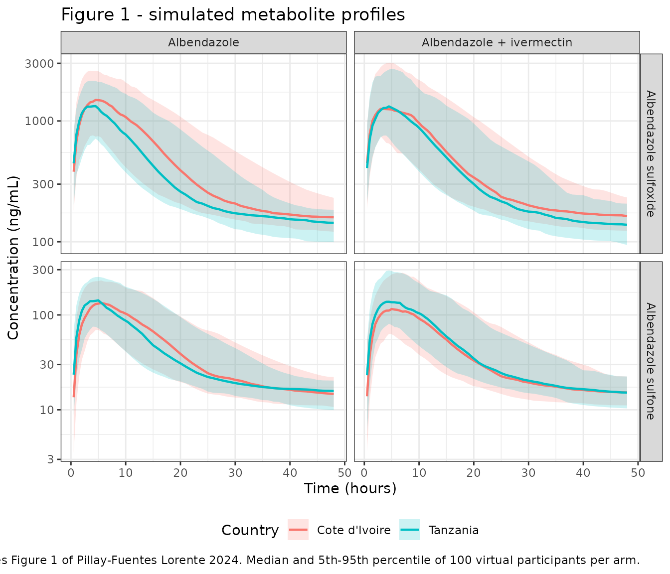
The two medication columns are identical by construction: co-medication was tested and rejected as a covariate (Results 3.3), so the model has no ivermectin term. This reproduces the paper’s headline negative result.
Figure 3 - visual predictive check by country
Fig. 3 shows prediction-corrected VPCs of both metabolite models in semi-log format, and Figs. S6-S7 of the ESM stratify them by country. Prediction correction requires the observed data, which are not public, so the panel below is an uncorrected simulated VPC stratified by country.
# Approximates Figure 3 / ESM Figures S6-S7 of Pillay-Fuentes Lorente 2024.
prof |>
  dplyr::filter(medication == "Albendazole") |>
  ggplot(aes(time, Q50)) +
  geom_ribbon(aes(ymin = Q05, ymax = Q95), alpha = 0.25, fill = "steelblue") +
  geom_line(linewidth = 0.8) +
  facet_grid(analyte ~ country, scales = "free_y") +
  scale_y_log10() +
  labs(x = "Time (hours)", y = "Concentration (ng/mL)",
       title = "Figure 3 - simulated VPC stratified by country",
       caption = "Approximates Figure 3 (and ESM Figures S6-S7) of Pillay-Fuentes Lorente 2024.") +
  theme_bw()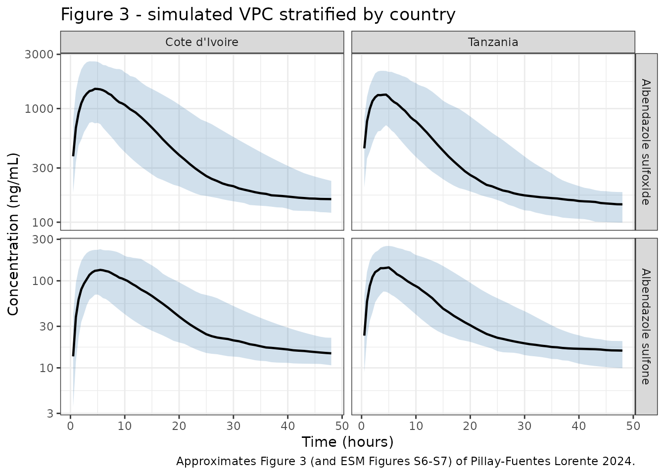
Figure S9 - simulated AUC(0-48 h) by country
Results 3.5 states: “The median of simulated AUC from 0 to 48 h was slightly lower in Tanzania than Cote d’Ivoire, which is in line with the higher clearance seen in Tanzania.” That is the one quantitative claim attached to the model-based simulations, so it is a direct validation target. ESM Fig. S9 was not available, so only the direction and rough magnitude can be checked.
The country contrast is simulated with common random
numbers: the same 200 virtual participants are solved twice,
once with REGION_TANZANIA = 0 and once with
REGION_TANZANIA = 1, so every subject is its own control
and the comparison carries no Monte Carlo noise. Drawing two independent
cohorts would blur a roughly 10% covariate signal behind sampling
variation in the median.
# Replicates ESM Figure S9 of Pillay-Fuentes Lorente 2024 (AUC0-48 by country).
paired_n <- 200L

make_paired <- function(region_tanzania, country) {
  subj <- tibble::tibble(id = seq_len(paired_n),
                         REGION_TANZANIA = region_tanzania,
                         country = country)
  dplyr::bind_rows(
    subj |> dplyr::mutate(time = 0, amt = 400, evid = 1L,
                          cmt = "depot", dvid = NA_integer_),
    subj |> tidyr::crossing(time = obs_times) |>
      dplyr::mutate(amt = NA_real_, evid = 0L, cmt = "central", dvid = 1L),
    subj |> tidyr::crossing(time = obs_times) |>
      dplyr::mutate(amt = NA_real_, evid = 0L, cmt = "central_abzson", dvid = 2L)
  ) |>
    dplyr::arrange(id, time)
}

solve_paired <- function(region_tanzania, country) {
  # Reseed INSIDE the helper so both country solves draw the identical etas.
  rxode2::rxSetSeed(20240722)
  set.seed(20240722)
  rxode2::rxSolve(mod, events = make_paired(region_tanzania, country),
                  keep = c("country", "REGION_TANZANIA"),
                  useLinCmt = FALSE) |>
    as.data.frame() |>
    dplyr::distinct(id, time, .keep_all = TRUE) |>
    dplyr::mutate(id = as.integer(as.character(id)))
}

sim_paired <- dplyr::bind_rows(
  solve_paired(0L, "Cote d'Ivoire"),
  solve_paired(1L, "Tanzania")
)

# The paired design is only valid if the two solves really did share etas:
# with common random numbers every subject's cl ratio must equal exp(0.56)
# exactly, and every cl_abzson ratio must equal exp(0.38) exactly.
ratio_check <- sim_paired |>
  dplyr::distinct(id, country, cl, cl_abzson) |>
  tidyr::pivot_wider(id_cols = id, names_from = country,
                     values_from = c(cl, cl_abzson))
stopifnot(
  nrow(ratio_check) == paired_n,
  max(abs(ratio_check$`cl_Tanzania` /
            ratio_check$`cl_Cote d'Ivoire` - exp(0.56))) < 1e-8,
  max(abs(ratio_check$`cl_abzson_Tanzania` /
            ratio_check$`cl_abzson_Cote d'Ivoire` - exp(0.38))) < 1e-8
)

auc48 <- sim_paired |>
  dplyr::group_by(id, country) |>
  dplyr::arrange(time, .by_group = TRUE) |>
  dplyr::summarise(
    auc_sox = 1000 * sum(diff(time) * (head(Cc, -1) + tail(Cc, -1)) / 2),
    auc_son = 1000 * sum(diff(time) * (head(Cc_abzson, -1) + tail(Cc_abzson, -1)) / 2),
    .groups = "drop"
  )

auc48_long <- auc48 |>
  tidyr::pivot_longer(c(auc_sox, auc_son),
                      names_to = "analyte", values_to = "auc") |>
  dplyr::mutate(analyte = ifelse(analyte == "auc_sox",
                                 "Albendazole sulfoxide", "Albendazole sulfone"))

ggplot(auc48_long, aes(country, auc, fill = country)) +
  geom_boxplot(alpha = 0.6, outlier.size = 0.6) +
  facet_wrap(~analyte, scales = "free_y") +
  scale_y_log10() +
  labs(x = NULL, y = "AUC(0-48 h) (ng*h/mL)",
       title = "Figure S9 - simulated AUC(0-48 h) by country",
       caption = "Replicates ESM Figure S9 of Pillay-Fuentes Lorente 2024.") +
  theme_bw() +
  theme(legend.position = "none")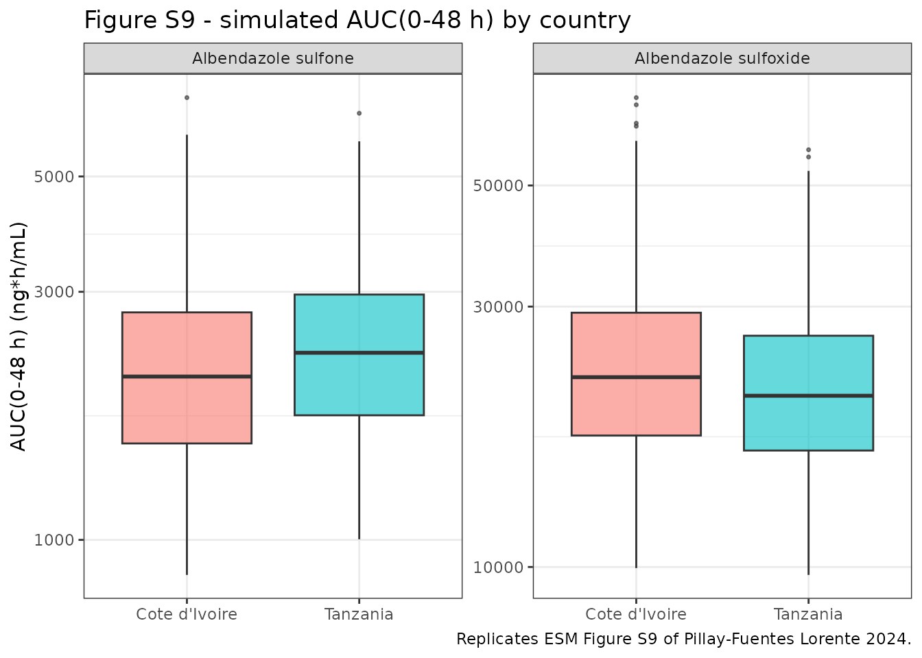
auc48_long |>
  tidyr::pivot_wider(id_cols = c(id, analyte),
                     names_from = country, values_from = auc) |>
  dplyr::group_by(analyte) |>
  dplyr::summarise(
    `Median AUC, Cote d'Ivoire (ng*h/mL)` = round(median(`Cote d'Ivoire`)),
    `Median AUC, Tanzania (ng*h/mL)`      = round(median(Tanzania)),
    `Median within-subject ratio (TZA/CIV)` =
      round(median(Tanzania / `Cote d'Ivoire`), 3),
    .groups = "drop"
  ) |>
  dplyr::rename(Analyte = analyte) |>
  knitr::kable(caption = paste(
    "Simulated AUC(0-48 h) by country, from",
    paired_n,
    "virtual participants solved under both country settings with common random numbers."
))| Analyte | Median AUC, Cote d’Ivoire (ng*h/mL) | Median AUC, Tanzania (ng*h/mL) | Median within-subject ratio (TZA/CIV) |
|---|---|---|---|
| Albendazole sulfone | 2173 | 2405 | 1.105 |
| Albendazole sulfoxide | 23650 | 21654 | 0.921 |
For albendazole sulfoxide the simulated median AUC(0-48 h) is lower in Tanzania, matching Results 3.5. For albendazole sulfone the model predicts the opposite direction; see the Errata section below, which works through why the published structure necessarily implies this.
PKNCA validation
NCA is run separately for each of the two model outputs, grouped by country so the per-country contrast can be read directly. The paper reports no NCA table of its own, so the comparison targets below are the model-implied exposure identities and the concentration ranges visible in Fig. 1.
nca_one <- function(sim_df, conc_col) {
  # select-with-rename in one step: renaming in place would collide with the
  # sibling observable column that is already called Cc.
  conc <- sim_df |>
    dplyr::select(id, time, country, Cc = dplyr::all_of(conc_col)) |>
    dplyr::filter(!is.na(Cc))

  # Guarantee a time = 0 row per (id, country); pre-dose extravascular Cc = 0.
  conc <- dplyr::bind_rows(
    conc,
    conc |> dplyr::distinct(id, country) |> dplyr::mutate(time = 0, Cc = 0)
  ) |>
    dplyr::distinct(id, country, time, .keep_all = TRUE) |>
    dplyr::arrange(id, country, time)

  dose_df <- events |>
    dplyr::filter(evid == 1L) |>
    dplyr::select(id, time, amt, country)

  intervals <- data.frame(
    start = 0, end = 48,
    cmax = TRUE, tmax = TRUE, auclast = TRUE, half.life = TRUE
  )

  PKNCA::pk.nca(PKNCA::PKNCAdata(
    PKNCA::PKNCAconc(conc, Cc ~ time | country + id),
    PKNCA::PKNCAdose(dose_df, amt ~ time | country + id),
    intervals = intervals
  ))
}

nca_sox <- nca_one(sim_wide, "Cc")
nca_son <- nca_one(sim_wide, "Cc_abzson")
summarise_nca <- function(res, analyte) {
  as.data.frame(res) |>
    dplyr::filter(PPTESTCD %in% c("cmax", "tmax", "auclast", "half.life")) |>
    dplyr::group_by(country, PPTESTCD) |>
    dplyr::summarise(median = median(PPORRES, na.rm = TRUE), .groups = "drop") |>
    dplyr::mutate(
      analyte = analyte,
      # Cc is in mg/L; report cmax and auclast in the paper's ng/mL units.
      median = dplyr::if_else(PPTESTCD %in% c("cmax", "auclast"),
                              1000 * median, median)
    )
}

nca_tbl <- dplyr::bind_rows(
  summarise_nca(nca_sox, "Albendazole sulfoxide"),
  summarise_nca(nca_son, "Albendazole sulfone")
) |>
  dplyr::mutate(PPTESTCD = factor(
    PPTESTCD,
    levels = c("cmax", "tmax", "auclast", "half.life"),
    labels = c("Cmax (ng/mL)", "Tmax (h)", "AUC(0-48 h) (ng*h/mL)", "t1/2 (h)")
  )) |>
  tidyr::pivot_wider(names_from = country, values_from = median) |>
  dplyr::arrange(analyte, PPTESTCD) |>
  dplyr::rename(Analyte = analyte, "NCA parameter" = PPTESTCD)

nca_tbl |>
  knitr::kable(digits = 2,
caption = "Median PKNCA parameters over 0-48 h by analyte and country.")| NCA parameter | Analyte | Cote d’Ivoire | Tanzania |
|---|---|---|---|
| Cmax (ng/mL) | Albendazole sulfone | 129.00 | 150.08 |
| Tmax (h) | Albendazole sulfone | 5.50 | 4.50 |
| AUC(0-48 h) (ng*h/mL) | Albendazole sulfone | 2246.10 | 2229.17 |
| t1/2 (h) | Albendazole sulfone | 197.07 | 254.95 |
| Cmax (ng/mL) | Albendazole sulfoxide | 1486.23 | 1397.26 |
| Tmax (h) | Albendazole sulfoxide | 4.50 | 4.00 |
| AUC(0-48 h) (ng*h/mL) | Albendazole sulfoxide | 24163.78 | 20810.26 |
| t1/2 (h) | Albendazole sulfoxide | 229.21 | 259.61 |
The simulated median albendazole sulfoxide Cmax is about 1400-1500 ng/mL and the sulfone Cmax about 130-150 ng/mL. Both sit slightly above the highest individual profiles visible in Fig. 1, which top out near 1000-1300 ng/mL for the sulfoxide and near 100 ng/mL for the sulfone. Two features of the design account for most of that gap, and neither is an encoding choice:
- Predicted Tmax is 4-4.5 h. Only the Ivorian schedule brackets it (1, 2, 4, 6, 8 h); the Tanzanian cohort’s first sample is at 6 h, already past the peak, so more than half the participants never observed a concentration near Tmax.
- The simulated cohort is sampled on a dense 0.5 h grid, so its Cmax is the true model maximum, whereas an observed Cmax can only ever be the largest of a handful of scheduled draws.
Nothing was tuned to close the gap: every value is exactly as
tabulated in Table 2. The paper’s own goodness-of-fit evidence is the
prediction-corrected VPC of Fig. 3, which cannot be reproduced without
the observed data, so the fit quality itself is not checkable here -
only that the published parameters have been transcribed and coupled
correctly, which the Dose / CL identity below establishes
exactly.
The t1/2 column is the apparent terminal half-life over
the 0-48 h sampling window, not the model’s true terminal half-life. The
published peripheral volume Pvox/F = 1931.53 L against Clox/F = 2.09 L/h
implies a genuine terminal half-life of several hundred hours, which is
far outside the 48 h observation window the model was fitted to. The
paper explicitly acknowledges this identifiability problem (Discussion:
the differing sampling schedules and the fixed ka “could explain the
difficulty in estimating the volume of distribution for albendazole
sulfoxide”).
Exposure identity check: AUC(0-inf) = Dose / CL
For this structure both exposures have exact closed forms, which makes them a strict test of the encoding rather than a soft plausibility check:
- albendazole sulfoxide is eliminated only via
Clox, soAUC(0-inf)_sulfoxide = Dose / Clox; - the sulfone is formed quantitatively from that same elimination
flux, so the amount of sulfone formed equals the dose and
AUC(0-inf)_sulfone = Dose / Clon.
Both must hold separately in each country, so the check simultaneously validates the two-compartment sulfoxide disposition, the 100%-conversion coupling and the covariate encoding on both clearances.
mod_typ <- readModelDb("PillayFuentesLorente_2024_albendazole") |> rxode2::zeroRe()
#> ℹ parameter labels from comments will be replaced by 'label()'

# A long horizon with dense early sampling so lambda-z is estimated on the true
# terminal phase (the model's terminal half-life is several hundred hours).
long_times <- c(seq(0, 48, by = 0.25), seq(50, 3000, by = 10))

typ_subj <- tibble::tibble(
  id = c(1L, 2L),
  REGION_TANZANIA = c(0L, 1L),
  country = c("Cote d'Ivoire", "Tanzania"),
  medication = "Albendazole"
)

typ_events <- dplyr::bind_rows(
  typ_subj |>
    dplyr::mutate(time = 0, amt = 400, evid = 1L,
                  cmt = "depot", dvid = NA_integer_),
  typ_subj |>
    tidyr::crossing(time = long_times) |>
    dplyr::mutate(amt = NA_real_, evid = 0L, cmt = "central", dvid = 1L),
  typ_subj |>
    tidyr::crossing(time = long_times) |>
    dplyr::mutate(amt = NA_real_, evid = 0L, cmt = "central_abzson", dvid = 2L)
) |>
  dplyr::arrange(id, time)

sim_typ <- rxode2::rxSolve(mod_typ, events = typ_events,
                           keep = c("country", "REGION_TANZANIA"),
                           omega = NA, sigma = NA, useLinCmt = FALSE) |>
  as.data.frame() |>
  dplyr::distinct(id, time, .keep_all = TRUE) |>
  dplyr::mutate(id = as.integer(as.character(id)))

auc_inf <- function(df, col) {
  conc <- df |>
    dplyr::select(id, time, country, Cc = dplyr::all_of(col)) |>
    dplyr::filter(!is.na(Cc))
  dose_df <- typ_events |>
    dplyr::filter(evid == 1L) |>
    dplyr::select(id, time, amt, country)
  res <- PKNCA::pk.nca(PKNCA::PKNCAdata(
    PKNCA::PKNCAconc(conc, Cc ~ time | country + id),
    PKNCA::PKNCAdose(dose_df, amt ~ time | country + id),
    intervals = data.frame(start = 0, end = Inf, aucinf.obs = TRUE)
  ))
  as.data.frame(res) |>
    dplyr::filter(PPTESTCD == "aucinf.obs") |>
    dplyr::select(country, aucinf = PPORRES)
}

cl_civ <- 2.09
cl_tza <- 2.09 * exp(0.56)
cln_civ <- 22.87
cln_tza <- 22.87 * exp(0.38)

identity_tbl <- dplyr::bind_rows(
  auc_inf(sim_typ, "Cc") |>
    dplyr::mutate(Analyte = "Albendazole sulfoxide",
                  expected = 400 / c("Cote d'Ivoire" = cl_civ, "Tanzania" = cl_tza)[country]),
  auc_inf(sim_typ, "Cc_abzson") |>
    dplyr::mutate(Analyte = "Albendazole sulfone",
                  expected = 400 / c("Cote d'Ivoire" = cln_civ, "Tanzania" = cln_tza)[country])
) |>
  dplyr::transmute(
    Analyte,
    Country = country,
    `Simulated AUC(0-inf) (mg*h/L)` = round(aucinf, 3),
    `Dose / CL (mg*h/L)` = round(expected, 3),
    `Ratio` = round(aucinf / expected, 4)
  )

knitr::kable(identity_tbl,
caption = "Simulated AUC(0-inf) versus the exact Dose / CL identity implied by the published structure.")| Analyte | Country | Simulated AUC(0-inf) (mg*h/L) | Dose / CL (mg*h/L) | Ratio |
|---|---|---|---|---|
| Albendazole sulfoxide | Cote d’Ivoire | 191.333 | 191.388 | 0.9997 |
| Albendazole sulfoxide | Tanzania | 109.313 | 109.322 | 0.9999 |
| Albendazole sulfone | Cote d’Ivoire | 17.486 | 17.490 | 0.9997 |
| Albendazole sulfone | Tanzania | 11.960 | 11.961 | 1.0000 |
# Hard gate: the identity must hold to within numerical / lambda-z tolerance.
stopifnot(all(abs(identity_tbl$Ratio - 1) < 0.002))
Both analytes recover Dose / CL in both countries, so
the sulfoxide disposition, the quantitative sulfoxide-to-sulfone
coupling and the two country effects are all encoded as published.
Country contrast on clearance
sim_typ |>
  dplyr::distinct(country, cl, cl_abzson) |>
  tidyr::pivot_longer(c(cl, cl_abzson), names_to = "param", values_to = "value") |>
  tidyr::pivot_wider(names_from = country, values_from = value) |>
  # Bind the labels to the parameter BY NAME, never by row position.
  dplyr::mutate(
    Parameter = dplyr::case_match(param,
                                  "cl" ~ "Clox/F (L/h)",
                                  "cl_abzson" ~ "Clon/F (L/h)"),
    `Paper states` = dplyr::case_match(param,
                                       "cl" ~ "75% higher",
                                       "cl_abzson" ~ "46% higher"),
    `Fold-change (Tanzania / Cote d'Ivoire)` = round(Tanzania / `Cote d'Ivoire`, 4)
  ) |>
  dplyr::select(Parameter, `Cote d'Ivoire`, Tanzania,
                `Fold-change (Tanzania / Cote d'Ivoire)`, `Paper states`) |>
  knitr::kable(digits = 3,
               caption = "Typical-value apparent clearances by country, versus the paper's stated percentage differences.")
#> Warning: There was 1 warning in `dplyr::mutate()`.
#> ℹ In argument: `Parameter = dplyr::case_match(...)`.
#> Caused by warning:
#> ! `case_match()` was deprecated in dplyr 1.2.0.
#> ℹ Please use `recode_values()` instead.| Parameter | Cote d’Ivoire | Tanzania | Fold-change (Tanzania / Cote d’Ivoire) | Paper states |
|---|---|---|---|---|
| Clox/F (L/h) | 2.09 | 3.659 | 1.751 | 75% higher |
| Clon/F (L/h) | 22.87 | 33.442 | 1.462 | 46% higher |
Assumptions and deviations
Transit-compartment absorption is encoded at its limiting form
Monolix parameterises the Savic transit chain by the mean transit
time Mtt and the transit rate constant Ktr,
with the implied (non-integer) number of transit compartments
nn = Mtt * Ktr - 1 and a transit input that is a
Gamma(shape = nn + 1, rate = Ktr) density scaled by the
dose. At the published estimates the shape parameter is
Mtt * Ktr = 0.095 * 0.12 = 0.0114, i.e.
nn = -0.9886, just inside the nn > -1
support boundary.
That distribution is not literally a point mass - it has a long, thin tail - but it is overwhelmingly front-loaded relative to the sampling schedule:
shape <- 0.095 * 0.12   # Mtt * Ktr
rate  <- 0.12           # Ktr
tibble::tibble(
  `Time after dose (h)` = c(1e-4, 0.1, 1, 8, 27),
  `Fraction of dose out of transit` =
    round(pgamma(c(1e-4, 0.1, 1, 8, 27), shape = shape, rate = rate), 4)
) |>
  knitr::kable(caption = paste(
    "Cumulative arrival of the published Gamma(shape =", signif(shape, 3),
    ", rate =", rate, ") transit input. The earliest observation in either",
    "cohort is at 1 h."
))| Time after dose (h) | Fraction of dose out of transit |
|---|---|
| 0.0001 | 0.8845 |
| 0.1000 | 0.9569 |
| 1.0000 | 0.9812 |
| 8.0000 | 0.9973 |
| 27.0000 | 0.9999 |
88% of the dose has left the transit chain within 0.36 seconds and
98% within 1 h, the earliest observation in either cohort. The model
file therefore encodes the exact nn -> -1 limiting form
- the dose lands directly in depot, which absorbs at the
fixed ka - rather than calling rxode2’s
transit() builtin, for two reasons.
First, transit() cannot integrate the published
shape. The input density carries a t^nn
singularity at the dose time. Sweeping nn at the published
Mtt shows the solver succeeds down to
nn = -0.60 and fails at nn <= -0.65, well
above the published nn = -0.9886. (Guarding the singularity
with a small time offset does not rescue it: it silently truncates the
spike where most of the mass sits and loses about 90% of the dose.)
Second, the substitution is quantitatively
negligible. The check below is the honest one: it compares the
shipped encoding against a mass-conserving discretisation of the
exact published input, using both the published Mtt
and the published Ktr. (Comparing instead against
transit() at some larger integrable nn would
silently change Ktr, since rxode2 derives
ktr = (nn + 1) / Mtt, and so would not bound the published
case at all.)
# Typical-value (no IIV) Cote d'Ivoire subject, solved two ways.
mod_tr <- readModelDb("PillayFuentesLorente_2024_albendazole") |> rxode2::zeroRe()
#> ℹ parameter labels from comments will be replaced by 'label()'

tr_times <- c(seq(0, 12, by = 0.05), seq(12.5, 48, by = 0.5))

tr_events <- function(dose_tbl) {
  # Observation rows name the ODE STATES and carry the dvid selecting the
  # endpoint, exactly as in the simulation chunks above.
  dplyr::bind_rows(
    dose_tbl,
    tibble::tibble(id = 1L, REGION_TANZANIA = 0L, time = tr_times,
                   amt = NA_real_, evid = 0L, cmt = "central", dvid = 1L),
    tibble::tibble(id = 1L, REGION_TANZANIA = 0L, time = tr_times,
                   amt = NA_real_, evid = 0L, cmt = "central_abzson", dvid = 2L)
  ) |>
    dplyr::arrange(time)
}

# (a) shipped encoding: the whole dose enters `depot` at t = 0
ev_limit <- tr_events(tibble::tibble(
  id = 1L, REGION_TANZANIA = 0L, time = 0, amt = 400, evid = 1L,
  cmt = "depot", dvid = NA_integer_
))

# (b) exact input: lump the mass arriving before t0 at t = 0, then discretise
#     the remaining tail into equal-probability arrivals.
t0 <- 1e-3
p0 <- pgamma(t0, shape = shape, rate = rate)
K  <- 300L
tail_times <- qgamma(p0 + (seq_len(K) - 0.5) / K * (1 - p0),
                     shape = shape, rate = rate)

ev_exact <- tr_events(tibble::tibble(
  id = 1L, REGION_TANZANIA = 0L,
  time = c(0, tail_times),
  amt  = c(400 * p0, rep(400 * (1 - p0) / K, K)),
  evid = 1L, cmt = "depot", dvid = NA_integer_
))

solve_tr <- function(ev) {
  rxode2::rxSolve(mod_tr, events = ev, omega = NA, sigma = NA,
                  useLinCmt = FALSE) |>
    as.data.frame() |>
    dplyr::filter(time %in% tr_times) |>
    dplyr::distinct(time, .keep_all = TRUE)
}

lim <- solve_tr(ev_limit)
exa <- solve_tr(ev_exact)
stopifnot(nrow(lim) == nrow(exa), all(is.finite(exa$Cc)))

trap <- function(t, y) sum(diff(t) * (head(y, -1) + tail(y, -1)) / 2)
obs <- lim$time >= 1   # earliest observation in either cohort

transit_cmp <- tibble::tibble(
  Metric = c("Max relative difference in Cc, t >= 1 h",
             "Max relative difference in Cc_abzson, t >= 1 h",
             "Relative difference in sulfoxide Cmax",
             "Relative difference in sulfoxide AUC(0-48 h)",
             "Relative difference in sulfone AUC(0-48 h)"),
  `Difference (%)` = round(100 * c(
    max(abs(exa$Cc[obs] - lim$Cc[obs]) / lim$Cc[obs]),
    max(abs(exa$Cc_abzson[obs] - lim$Cc_abzson[obs]) / lim$Cc_abzson[obs]),
    abs(max(exa$Cc) - max(lim$Cc)) / max(lim$Cc),
    abs(trap(exa$time, exa$Cc) - trap(lim$time, lim$Cc)) / trap(lim$time, lim$Cc),
    abs(trap(exa$time, exa$Cc_abzson) - trap(lim$time, lim$Cc_abzson)) /
      trap(lim$time, lim$Cc_abzson)
  ), 3)
)

knitr::kable(transit_cmp, caption = paste(
  "Shipped limiting-form encoding versus a mass-conserving discretisation of the",
  "exact published Gamma transit input, at the published Mtt and Ktr."
))| Metric | Difference (%) |
|---|---|
| Max relative difference in Cc, t >= 1 h | 2.794 |
| Max relative difference in Cc_abzson, t >= 1 h | 3.186 |
| Relative difference in sulfoxide Cmax | 0.922 |
| Relative difference in sulfoxide AUC(0-48 h) | 0.066 |
| Relative difference in sulfone AUC(0-48 h) | 0.066 |
# Hard gate: the deviation must stay small at every observable time.
stopifnot(max(abs(exa$Cc[obs] - lim$Cc[obs]) / lim$Cc[obs]) < 0.05)
The deviation is at most a few percent at any time the study actually
observed, and well under 0.1% in AUC. The fixed
ka = 0.2 1/h remains the rate-limiting absorption step
either way.
Because nn does not enter any ODE in this encoding,
Ktr and Mtt have identically zero influence on
the predictions. They are retained in ini() at their
published values for provenance, but are wrapped in fixed()
so that re-estimating this model does not produce a structurally
singular problem. The paper did estimate both (RSE 6.01% and 8.72%);
that status is recorded in the model file’s in-line comments and in the
source-trace table above.
Sulfone exposure is predicted to be higher in Tanzania
Results 3.5 says the median simulated AUC(0-48 h) “was slightly lower in Tanzania than Cote d’Ivoire, which is in line with the higher clearance seen in Tanzania”, and refers to ESM Fig. S9 “for both metabolites”. The simulations above reproduce that for albendazole sulfoxide but give the opposite direction for albendazole sulfone.
This is forced by the published structure, not by a transcription
choice. Because conversion is quantitative, the sulfone formation flux
is Clox * C_sulfoxide, so total sulfone formed equals the
dose regardless of Clox, and
AUC_sulfone = Dose / Clon. Raising Clox by 75%
raises the sulfone formation rate while leaving the total
amount formed unchanged; only the 46% higher Clon then acts
on the exposure. Over the truncated 0-48 h window the net effect is a
roughly 10% higher sulfone AUC in Tanzania (the sulfoxide AUC
falls to 0.92 of the Ivorian value, the formation clearance rises
1.75-fold and the sulfone clearance rises 1.46-fold:
0.92 * 1.75 / 1.46 = 1.10).
ESM Fig. S9 was not available, so it cannot be checked directly. Either the Results 3.5 sentence describes only the sulfoxide panel, or the published simulation differs from the tabulated final model in a way that is not recoverable from the article text. Nothing was tuned to remove the discrepancy.
Errata and reporting issues in the source
- Duplicated residual-error row label. Table 2 lists both residual-variability rows as “Sulfoxide, proportional” (0.43 and 0.22). The model has exactly two outputs and every other block of Table 2 lists the sulfoxide entry before the sulfone entry, so the second row is taken as the albendazole sulfone proportional error. The 0.43 / 0.22 split is also consistent with Fig. 1, where the sulfoxide profiles are visibly more scattered than the sulfone profiles.
-
“CP” versus “CC” in the random-effects block. Table
2’s random-effect rows say “in the CP” for
omega(Vox),omega(Von)andomega(Clox), but the table’s own footnote defines CC = central compartment and PC = peripheral compartment, andVonis defined in the population block as the sulfone volume “in the CC”. The only row that genuinely refers to the peripheral compartment isomega(Pvox), which spells it “PC”. The first three are read as central- compartment (and, foromega(Clox), simply clearance) random effects. -
Absorption rate constant provenance.
kawas fixed at 0.2 1/h “based on the estimate from a previous model (unpublished data)” (Results 3.2). The value itself is published in Table 2, so nothing had to be sourced off-paper, but it is not an estimate from these data.
Other assumptions
- No molar-mass conversion. The paper assumes 100% conversion on a mass-amount basis and reports apparent (F-relative) volumes and clearances estimated on that basis, so the 400 mg albendazole dose is carried through the chain unchanged rather than being converted to sulfoxide- or sulfone-equivalent mass.
-
Omega scale. Monolix reports
omegaas the standard deviation of the log-scale random effect for log-normally distributed parameters (Methods 2.2), so the nlmixr2 variances areomega^2. No CV%-to-variance conversion is involved. -
No IIV on
Ktr,MttorClon. Table 2 reports none, and none was invented. -
Covariates screened but not retained. Body weight,
body mass index, sex and co-administered ivermectin were all tested and
rejected (Results 3.3). They are recorded in the model file’s
covariatesDataExcludedmetadata rather than incovariateData, sincemodel()does not reference them. - Sensitivity analysis excluded. The paper’s sensitivity analysis (Results 3.4, ESM Table S1), which refits after excluding Tanzanian samples beyond 27 h with the peripheral parameters fixed, is a robustness check rather than the published final model and is not extracted.
- Exploratory exposure-efficacy analysis not extracted. Section 3.6 and Fig. 4 relate Cpeak and time-above-threshold to the relative egg count, but the analysis is explicitly exploratory: it reports grouped scatter plots with trend lines and no fitted model, no parameter estimates and no equation. There is nothing to encode.
- Supplement not available. ESM Figs. S1-S9 and Table S1 were not available when this model was built. They contain goodness-of-fit plots, VPCs, the AUC-by-country figure and the sensitivity-analysis parameter table - none of which are needed for the final model, whose parameters are all in Table 2.
- Virtual cohort demographics. No covariate other than country enters the model, so the virtual cohorts carry only the country indicator; the age, weight and sex distributions of Table 1 are not needed to simulate from the published model.