SNX-2112 cosolvent and nanocrystal rat PBPK (Dong 2015)
Source:vignettes/articles/Dong_2015_snx2112_nanocrystals.Rmd
Dong_2015_snx2112_nanocrystals.RmdModel and source
Citation: Dong D, Wang X, Wang H, Zhang X, Wang Y, Wu B. Elucidating the in vivo fate of nanocrystals using a physiologically based pharmacokinetic model: a case study with the anticancer agent SNX-2112. Int J Nanomedicine. 2015;10:2521-2535. doi:10.2147/IJN.S79734
Article: Int J Nanomedicine. 2015;10:2521-2535 (open access, PMC4386773)
SNX-2112 is a heat-shock-protein-90 inhibitor that is poorly soluble in both water and oil. Dong and colleagues milled it into 203 nm nanocrystals stabilised with poloxamer 188, dosed rats intravenously with either the nanocrystals or a 45% propylene-glycol cosolvent solution (2 mg/kg), measured SNX-2112 in plasma and six tissues, and built two whole-body physiologically based pharmacokinetic (PBPK) models in MATLAB:
| Model | Arm | Equations | Estimated in this arm |
|---|---|---|---|
| Dong_2015_snx2112_rat_pbpk | Cosolvent (dissolved drug) | Eqs 1-8 | Kp,li, Kp,lu, Kp,rm, CLH |
| Dong_2015_snx2112_nanocrystal_rat_pbpk | Nanocrystals | Eqs 9-19 | Upli, Upsp, Krel (all nonparticulate parameters fixed) |
The nonparticulate model (Figure 1A) is a perfusion-limited network
of plasma, heart, spleen, intestine, kidney, liver, lung and a lumped
remainder. The spleen and intestine drain into the liver; the liver,
heart, kidney and remainder drain into the lung, which returns to plasma
at the plasma cardiac output. Elimination is hepatic only. The
nanoparticulate model (Figure 1B) adds a nanocrystal species in plasma,
liver and spleen: particles are taken up from plasma into the liver and
spleen by the apparent clearances Upli and
Upsp, and dissolve by the first-order constant
Krel.
Read the Errata before using these models. The published parameter set does not reproduce the paper’s own tissue data (lung by about 200-fold, liver and systemic clearance by up to about 1.7-fold), and the printed release term does not reproduce the paper’s own Figure 9 simulation. Both models encode the published equations and Table 4 values as printed; nothing has been re-fitted.
Population
Male Sprague-Dawley rats, 193.0 +/- 8.9 g (Methods, “Pharmacokinetic study of SNX-2112”). Each arm received 2 mg/kg intravenously by the tail vein. Sampling was destructive: five rats per time at 10, 20 and 30 min and 1, 2, 4, 6, 8, 12 and 18 h, with blood (cardiac puncture) and heart, liver, spleen, lung, kidney and intestine collected from each, so 50 rats per arm. SNX-2112 was measured by UPLC-QTOF/MS (linear range 4.88-5000 nM). The models were fitted to the arm means by weighted least squares (1/y^2 weights).
The physiology (Table 1) is for a 250 g rat, not the 193 g animals studied. The dose the authors used in their analysis is also the 250 g one: Table 2’s two-compartment clearance equals that dose over Table 2’s AUC(0-inf) exactly (checked below).
Source trace
| Quantity | Value | Source |
|---|---|---|
| Nonparticulate ODEs | Eqs 1-8 | Methods, “Nonparticulate PBPK model” (p. 2524) |
| Nanoparticulate ODEs | Eqs 9-19 | Methods, “Nanoparticulate PBPK model” (p. 2525) |
qc (Qco) |
2.69 L/h | Methods text; Table 1 lung row |
q_liver, q_kidney, q_spleen,
q_intestine, q_heart,
q_other
|
0.4920, 0.3790, 0.0269, 0.3850, 0.1320, 1.2800 L/h | Table 1 |
v_liver, v_kidney, v_spleen,
v_intestine, v_lung, v_heart,
v_other
|
0.009150, 0.001830, 0.000500, 0.006750, 0.001250, 0.000825, 0.221000 L | Table 1 |
v_plasma |
0.008695 L | Not printed; Table 1 residual (see Plasma volume) |
lkp_kidney, lkp_spleen,
lkp_intestine, lkp_heart
|
log(5.92), log(6.78), log(12.2), log(2.24) | Table 4, fixed (footnote b); Figure 6 |
lkp_liver, lkp_lung,
lkp_other
|
log(4.03), log(0.0213), log(5.15) | Table 4, estimated (footnote a) |
lclh |
log(0.0246 L/h) | Table 4, estimated (footnote a) |
lclup_liver, lclup_spleen
|
log(0.0906), log(0.182) L/h | Table 4 (nanocrystal arm) |
lkrel |
log(0.0257 1/h) | Table 4 (nanocrystal arm) |
| Dose | 2 mg/kg x 0.250 kg = 0.5 mg = 1.0764 umol | Methods; Table 1 caption (250 g); molecular weight 464.5 g/mol (C23H27F3N4O3, not printed in the paper) |
| Observation | plasma total SNX-2112, uM | Methods; Figure 9 (“Total drug = nonparticulate + nanoparticulate drug”) |
Table 1 cites reference 42, a bioanalytical paper. The values are those of reference 43 (Kagan et al. 2011, AAPS J 13:255, Table I, rat): plasma flows of 18.3, 14.1, 1.0, 14.3 and 4.9% of cardiac output for liver, kidney, spleen, gastrointestinal tract and heart, and tissue volumes of 3.66, 0.73, 0.2, 2.7, 0.33 and 0.5% of body weight for liver, kidney, spleen, gastrointestinal tract, heart and lungs. Multiplied by 2.69 L/h and 0.250 kg these give every Table 1 row.
Hepatic flow
Eqs 7 and 17 bring plasma into the liver at the hepatic-artery flow
Qha, and Eqs 7, 8, 17 and 19 take it out at
Qli. Table 1 prints a single liver flow, 0.4920 L/h. The
maintainers encode that single printed value for both
symbols. Two other readings were considered:
-
Qha = 0.4920 - Qsp - Qin = 0.0801withQli = 0.4920. The paper’s own arithmetic rules this out: the Table 1 remainder flow, 1.28 L/h, isQco - (0.4920 + 0.3790 + 0.0269 + 0.3850 + 0.1320) = 1.275, which deducts the full 0.4920 as flow drawn directly from plasma. Under this reading the plasma equation would also lose 0.41 L/h of flow that no tissue receives. -
Qha = 0.4920withQli = Qha + Qsp + Qin = 0.9039. This is the physiologically coherent reading (liver outflow equals liver inflow), but it scores worst against the paper’s anchors: systemic clearance 0.084 L/h against an observed 0.256 L/h (0.15 L/h with the encoded reading), and, with the release term written asKrel x C(see Figure 9), a plasma curve 2.4-fold above Figure 9A at 10 h against 1.4-fold for the encoded reading.
With Qha = Qli = 0.4920 the network is close to globally
mass-conservative: the tissues draw 2.6949 L/h from plasma against the
2.69 L/h that Eq 1 removes, a 0.0049 L/h rounding mismatch in Table 1
that is checked below.
Plasma volume
Every plasma equation divides by the plasma volume Vpl,
which is printed nowhere in the paper or in Kagan 2011. Table 1’s
“Remaining” volume is a residual of the 250 g rat, the same construction
that gives its remainder flow, so
Vpl = 0.250 - 0.221000 - (0.009150 + 0.001830 + 0.000500 + 0.006750 + 0.001250 + 0.000825) = 0.008695 L
(34.8 mL/kg). Figure 9A independently supports it: its
nanoparticulate plasma curve is clipped at the 100 uM top of the axis
and back-extrapolates to about 117 uM at time zero, against
Dose / Vpl = 1.0764 / 0.008695 = 124 uM.
Simulation
Both models are deterministic, so a single typical rat per arm is simulated.
mw_snx2112 <- 464.5 # g/mol, C23H27F3N4O3
dose_umol <- 2 * 0.250 / mw_snx2112 * 1000 # 2 mg/kg x 250 g rat

mod_cos <- rxode2::rxode(readModelDb("Dong_2015_snx2112_rat_pbpk"))
mod_nano <- rxode2::rxode(readModelDb("Dong_2015_snx2112_nanocrystal_rat_pbpk"))

obs_times <- sort(unique(c(seq(0, 1, by = 0.0025), seq(1, 18, by = 0.025))))

ev_cos <- rxode2::et(amt = dose_umol, cmt = "plasma") |>
  rxode2::et(obs_times)
ev_nano <- rxode2::et(amt = dose_umol, cmt = "plasma_np") |>
  rxode2::et(obs_times)

sim_cos <- rxode2::rxSolve(mod_cos, ev_cos, returnType = "data.frame")
sim_nano <- rxode2::rxSolve(mod_nano, ev_nano, returnType = "data.frame")

tissue_long <- function(sim, arm, nano) {
  data.frame(
    arm = arm,
    time = sim$time,
    plasma = sim$Cc,
    heart = sim$c_heart,
    liver = if (nano) sim$c_liver_total else sim$c_liver,
    spleen = if (nano) sim$c_spleen_total else sim$c_spleen,
    lung = sim$c_lung,
    kidney = sim$c_kidney,
    intestine = sim$c_intestine
  ) |>
    tidyr::pivot_longer(
      plasma:intestine,
      names_to = "tissue",
      values_to = "Cc"
    )
}

sim_long <- dplyr::bind_rows(
  tissue_long(sim_cos, "Cosolvent", nano = FALSE),
  tissue_long(sim_nano, "Nanocrystals", nano = TRUE)
)
sim_long |>
  dplyr::filter(time > 0) |>
  ggplot(aes(time, Cc, colour = arm)) +
  geom_line() +
  facet_wrap(~tissue, scales = "free_y") +
  scale_y_log10() +
  labs(
    x = "Time (h)",
    y = "SNX-2112 (uM)",
    colour = NULL,
    title = "Typical-value profiles, 2 mg/kg IV",
    caption = "Models as published (Table 4). Liver and spleen are total drug in the nanocrystal arm."
  )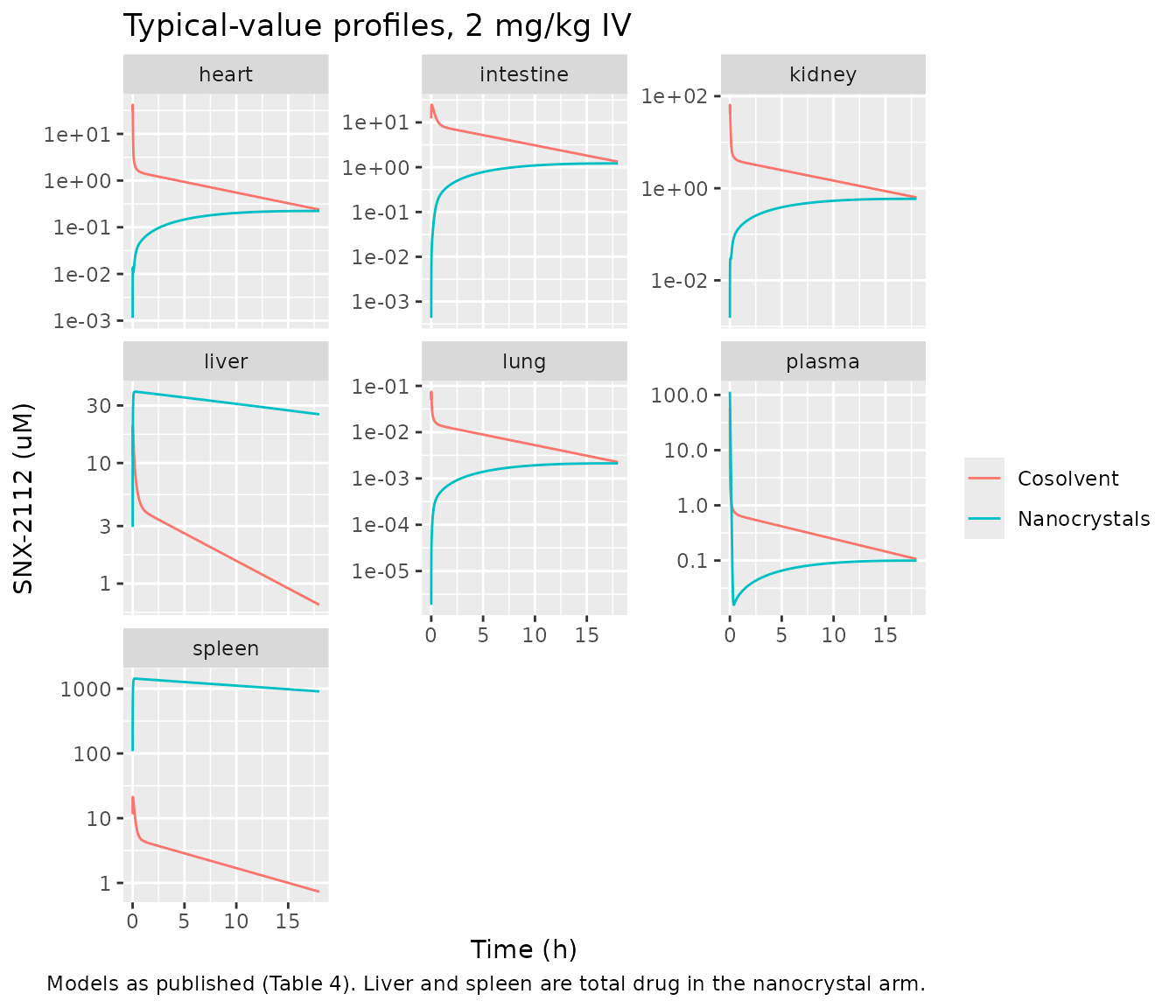
The nanocrystal liver and spleen curves show the defect of the
printed release term discussed in the Errata:
particles taken up by the spleen dissolve at
Krel = 0.0257 1/h, so the spleen holds about 1400 uM of
nanocrystalline drug at 30 min, still about 900 uM at 18 h.
Replicates Figure 9 of Dong 2015
Figure 9 is the authors’ own simulation of the nanocrystal arm, split into dissolved (nonparticulate), nanoparticulate and total drug in plasma, liver and spleen. It is a vector graphic, so the maintainers digitised it from the curve paths of the PDF; the values below are read off those paths at fixed times (the panel insets supply the first half hour).
# Digitised from the vector paths of Figure 9 (uM).
fig9 <- tibble::tribble(
  ~tissue, ~species, ~time, ~conc,
  "plasma", "total", 0.02, 61,
  "plasma", "total", 0.05, 22.15,
  "plasma", "total", 0.1, 5.089,
  "plasma", "total", 0.15, 1.562,
  "plasma", "total", 0.2, 0.8697,
  "plasma", "total", 0.3, 0.7218,
  "plasma", "total", 0.5, 0.6933,
  "plasma", "nonparticulate", 0.02, 0.7735,
  "plasma", "nonparticulate", 0.05, 1.341,
  "plasma", "nonparticulate", 0.1, 1.143,
  "plasma", "nonparticulate", 0.15, 0.8442,
  "plasma", "nonparticulate", 0.2, 0.7384,
  "plasma", "nonparticulate", 0.3, 0.6907,
  "plasma", "nonparticulate", 0.5, 0.6893,
  "plasma", "nanoparticulate", 0.02, 59.6,
  "plasma", "nanoparticulate", 0.05, 21.2,
  "plasma", "nanoparticulate", 0.1, 3.791,
  "plasma", "nanoparticulate", 0.15, 0.7007,
  "plasma", "nanoparticulate", 0.2, 0.1208,
  "spleen", "total", 0.02, 367,
  "spleen", "total", 0.05, 264,
  "spleen", "total", 0.1, 71.61,
  "spleen", "total", 0.15, 19.21,
  "spleen", "total", 0.2, 7.378,
  "spleen", "total", 0.3, 4.864,
  "spleen", "total", 0.5, 4.796,
  "spleen", "nonparticulate", 0.02, 6.581,
  "spleen", "nonparticulate", 0.05, 10.24,
  "spleen", "nonparticulate", 0.1, 7.931,
  "spleen", "nonparticulate", 0.15, 5.651,
  "spleen", "nonparticulate", 0.2, 5.013,
  "spleen", "nonparticulate", 0.3, 4.819,
  "spleen", "nonparticulate", 0.5, 4.827,
  "spleen", "nanoparticulate", 0.02, 373.9,
  "spleen", "nanoparticulate", 0.05, 261.4,
  "spleen", "nanoparticulate", 0.1, 65.08,
  "spleen", "nanoparticulate", 0.15, 13.94,
  "spleen", "nanoparticulate", 0.2, 2.452,
  "plasma", "total", 1, 0.664,
  "plasma", "total", 2, 0.5742,
  "plasma", "total", 4, 0.4172,
  "plasma", "total", 6, 0.3024,
  "plasma", "total", 8, 0.2175,
  "plasma", "total", 12, 0.1147,
  "plasma", "total", 16, 0.06056,
  "liver", "total", 0.25, 28.5,
  "liver", "total", 0.5, 16.64,
  "liver", "total", 1, 8.54,
  "liver", "total", 1.5, 6.235,
  "liver", "total", 2, 5.275,
  "liver", "total", 4, 3.726,
  "liver", "total", 6, 2.718,
  "liver", "total", 8, 1.955,
  "liver", "total", 12, 1.029,
  "liver", "total", 16, 0.5365,
  "liver", "nonparticulate", 0.25, 6.58,
  "liver", "nonparticulate", 0.5, 6.313,
  "liver", "nonparticulate", 1, 6.069,
  "liver", "nonparticulate", 1.5, 5.582,
  "liver", "nonparticulate", 2, 5.202,
  "liver", "nonparticulate", 4, 3.736,
  "liver", "nonparticulate", 6, 2.734,
  "liver", "nonparticulate", 8, 1.961,
  "liver", "nonparticulate", 12, 1.024,
  "liver", "nonparticulate", 16, 0.5357,
  "liver", "nanoparticulate", 0.25, 21.78,
  "liver", "nanoparticulate", 0.5, 10.74,
  "liver", "nanoparticulate", 1, 2.599,
  "liver", "nanoparticulate", 1.5, 0.6086,
  "liver", "nanoparticulate", 2, 0.1566,
  "spleen", "total", 1, 4.512,
  "spleen", "total", 2, 3.914,
  "spleen", "total", 4, 2.829,
  "spleen", "total", 6, 2.039,
  "spleen", "total", 8, 1.485,
  "spleen", "total", 12, 0.7727,
  "spleen", "total", 16, 0.4103,
  "spleen", "nonparticulate", 1, 4.521,
  "spleen", "nonparticulate", 2, 3.878,
  "spleen", "nonparticulate", 4, 2.804,
  "spleen", "nonparticulate", 6, 2.026,
  "spleen", "nonparticulate", 8, 1.482,
  "spleen", "nonparticulate", 12, 0.7709,
  "spleen", "nonparticulate", 16, 0.4083
)
The model as printed is compared with one alternative: the release
flux written as Krel x C (Krel acting as a clearance, in
L/h) instead of the printed Krel x V x C (Krel a rate
constant in 1/h). The alternative is built in the vignette by model
piping; it is not a packaged model.
mod_nano_krel_cl <- mod_nano |>
  rxode2::model({
    rel_plasma <- krel * c_plasma_np
    rel_spleen <- krel * c_spleen_np
    rel_liver <- krel * c_liver_np
  })
sim_nano_cl <- rxode2::rxSolve(
  mod_nano_krel_cl,
  ev_nano,
  returnType = "data.frame"
)

species_long <- function(sim, variant) {
  data.frame(
    variant = variant,
    time = sim$time,
    plasma.nonparticulate = sim$c_plasma,
    plasma.nanoparticulate = sim$c_plasma_np,
    liver.nonparticulate = sim$c_liver,
    liver.nanoparticulate = sim$c_liver_np,
    spleen.nonparticulate = sim$c_spleen,
    spleen.nanoparticulate = sim$c_spleen_np
  ) |>
    tidyr::pivot_longer(-c(variant, time), values_to = "conc") |>
    tidyr::separate(name, c("tissue", "species"), sep = "\\.") |>
    dplyr::bind_rows(
      data.frame(
        variant = variant,
        time = sim$time,
        tissue = rep(c("plasma", "liver", "spleen"), each = nrow(sim)),
        species = "total",
        conc = c(sim$Cc, sim$c_liver_total, sim$c_spleen_total)
      )
    )
}

fig9_sim <- dplyr::bind_rows(
  species_long(sim_nano, "As printed (Krel x V x C)"),
  species_long(sim_nano_cl, "Krel x C")
)

# Each variant's prediction at the digitised points (log-linear interpolation
# of the simulated curve).
predict_at <- function(sim_variant, tis, sp, t) {
  s <- sim_variant[sim_variant$tissue == tis & sim_variant$species == sp, ]
  exp(stats::approx(s$time, log(pmax(s$conc, 1e-12)), xout = t)$y)
}
fig9_err <- dplyr::bind_rows(lapply(
  split(fig9_sim, fig9_sim$variant),
  function(d) {
    fig9 |>
      dplyr::group_by(tissue, species) |>
      dplyr::mutate(pred = predict_at(d, tissue[1], species[1], time)) |>
      dplyr::ungroup() |>
      dplyr::mutate(variant = d$variant[1])
  }
))
fig9_score <- fig9_err |>
  dplyr::group_by(variant, tissue, species) |>
  dplyr::summarise(
    n = dplyr::n(),
    rms_log_error = sqrt(mean(log(pred / conc)^2)),
    .groups = "drop"
  )

fig9_score |>
  dplyr::mutate(
    rms_log_error = signif(rms_log_error, 2),
    `typical fold error` = signif(exp(rms_log_error), 2)
  ) |>
  dplyr::rename(
    Variant = variant,
    Tissue = tissue,
    Species = species,
    `Points` = n,
    `RMS log error` = rms_log_error
  ) |>
knitr::kable(caption = "Agreement with the digitised Figure 9 curves.")| Variant | Tissue | Species | Points | RMS log error | typical fold error |
|---|---|---|---|---|---|
| As printed (Krel x V x C) | liver | nanoparticulate | 5 | 3.300 | 27.0 |
| As printed (Krel x V x C) | liver | nonparticulate | 10 | 2.300 | 10.0 |
| As printed (Krel x V x C) | liver | total | 10 | 2.400 | 11.0 |
| As printed (Krel x V x C) | plasma | nanoparticulate | 5 | 0.410 | 1.5 |
| As printed (Krel x V x C) | plasma | nonparticulate | 7 | 4.700 | 110.0 |
| As printed (Krel x V x C) | plasma | total | 14 | 1.900 | 6.7 |
| As printed (Krel x V x C) | spleen | nanoparticulate | 5 | 3.800 | 45.0 |
| As printed (Krel x V x C) | spleen | nonparticulate | 14 | 1.500 | 4.5 |
| As printed (Krel x V x C) | spleen | total | 14 | 5.500 | 240.0 |
| Krel x C | liver | nanoparticulate | 5 | 0.100 | 1.1 |
| Krel x C | liver | nonparticulate | 10 | 0.510 | 1.7 |
| Krel x C | liver | total | 10 | 0.310 | 1.4 |
| Krel x C | plasma | nanoparticulate | 5 | 0.052 | 1.1 |
| Krel x C | plasma | nonparticulate | 7 | 0.480 | 1.6 |
| Krel x C | plasma | total | 14 | 0.330 | 1.4 |
| Krel x C | spleen | nanoparticulate | 5 | 0.055 | 1.1 |
| Krel x C | spleen | nonparticulate | 14 | 2.800 | 16.0 |
| Krel x C | spleen | total | 14 | 2.000 | 7.4 |
fig9_sim |>
  dplyr::filter(time > 0, conc > 1e-3) |>
  ggplot(aes(time, conc, colour = species)) +
  geom_line(aes(linetype = variant)) +
  geom_point(data = fig9, shape = 1) +
  facet_grid(tissue ~ ., scales = "free_y") +
  scale_y_log10() +
  scale_x_continuous(trans = "sqrt", breaks = c(0.1, 0.5, 1, 2, 4, 8, 12, 18)) +
  labs(
    x = "Time (h, square-root scale)",
    y = "SNX-2112 (uM)",
    colour = NULL,
    linetype = NULL,
    title = "Nanocrystal arm: published model vs Figure 9",
    caption = "Points: digitised from Figure 9 of Dong 2015. Lines: simulations."
  ) +
  theme(legend.position = "bottom", legend.box = "vertical")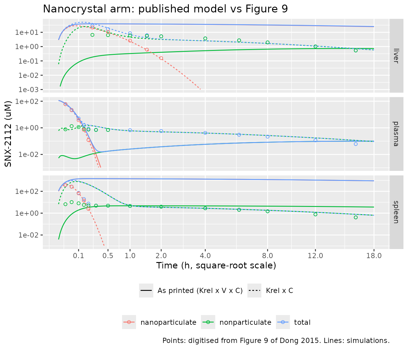
With Krel x C the three nanoparticulate curves of Figure
9 are reproduced to within about 10%: the particles leave plasma at
(Upli + Upsp) / Vpl + Krel / Vpl (about 34 1/h), the liver
at Krel / Vli (2.8 1/h) and the spleen at
Krel / Vsp (51 1/h), which is what the figure shows. As
printed, the release constants are Krel itself (0.0257 1/h,
a 27 h half-life) in every compartment, and the particles stay in the
liver and spleen. Neither variant reproduces the dissolved-drug curves
in the spleen, where Krel x C puts up to about 100 times
more dissolved drug than Figure 9 shows in the first half hour, so the
authors’ code differed from the printed equations in some further way
that the paper does not let us recover. See the Errata.
score <- function(v, tis, sp) {
  fig9_score$rms_log_error[
    fig9_score$variant == v & fig9_score$tissue == tis & fig9_score$species == sp
  ]
}
stopifnot(
  # Krel x C reproduces the particle kinetics the authors simulated.
  score("Krel x C", "plasma", "nanoparticulate") < 0.25,
  score("Krel x C", "liver", "nanoparticulate") < 0.25,
  score("Krel x C", "spleen", "nanoparticulate") < 0.25,
  # As printed, particles are retained in the liver and spleen: the error at
  # the digitised nanoparticulate points is more than 10-fold.
  score("As printed (Krel x V x C)", "liver", "nanoparticulate") > log(10),
  score("As printed (Krel x V x C)", "spleen", "nanoparticulate") > log(10)
)
Self-consistency checks
These checks confirm that the packaged models solve the printed equations correctly, independently of whether the printed parameters fit the data.
# (1) Dose convention. Table 2 (two-compartment fit, cosolvent): CL = 0.225
#     L/h and AUC(0-inf) = 4.79 uM*h. Dose / AUC reproduces CL only with the
#     250 g dose, confirming the dose used in the authors' analysis.
stopifnot(abs(dose_umol / 4.79 - 0.225) / 0.225 < 0.01)

# (2) Mass balance of the cosolvent model. The only sink is CLH * Cli; the
#     0.0049 L/h excess of tissue inflow over Qco is a source of
#     0.0049 * Cpl. Amount in the body + eliminated - created = dose.
ode_states <- c(
  "plasma", "heart", "spleen", "intestine", "other", "kidney", "liver", "lung"
)
cum_trapz <- function(t, y) c(0, cumsum(diff(t) * (head(y, -1) + tail(y, -1)) / 2))
q_sum <- 0.492 + 0.379 + 0.0269 + 0.385 + 0.132 + 1.28
mb <- rowSums(sim_cos[, ode_states]) +
  cum_trapz(sim_cos$time, 0.0246 * sim_cos$c_liver) -
  (q_sum - 2.69) * cum_trapz(sim_cos$time, sim_cos$Cc)
stopifnot(max(abs(mb - dose_umol)) / dose_umol < 1e-3)

# (3) Mass balance of the nanocrystal model, both variants.
nano_states <- c(ode_states, "plasma_np", "liver_np", "spleen_np")
for (s in list(sim_nano, sim_nano_cl)) {
  mb_nano <- rowSums(s[, nano_states]) +
    cum_trapz(s$time, 0.0246 * s$c_liver) -
    (q_sum - 2.69) * cum_trapz(s$time, s$c_plasma)
  stopifnot(max(abs(mb_nano - dose_umol)) / dose_umol < 1e-3)
}

# (4) Every fixed tissue Kp is reproduced as the simulated tissue:plasma
#     AUC(0-18 h) ratio, as it must be for a perfusion-limited tissue fed by
#     plasma once distribution has equilibrated.
auc018 <- function(t, y) tail(cum_trapz(t[t <= 18], y[t <= 18]), 1)
ratio <- function(col) auc018(sim_cos$time, sim_cos[[col]]) / auc018(sim_cos$time, sim_cos$Cc)
stopifnot(
  abs(ratio("c_heart") / 2.24 - 1) < 0.05,
  abs(ratio("c_kidney") / 5.92 - 1) < 0.05,
  abs(ratio("c_spleen") / 6.78 - 1) < 0.05,
  abs(ratio("c_intestine") / 12.2 - 1) < 0.10
)
PKNCA validation
AUC(0-18 h) in plasma and each tissue, per arm, computed by PKNCA from the typical-value profiles and compared with Table 3.
nca_conc <- sim_long |>
  dplyr::filter(!is.na(Cc)) |>
  dplyr::mutate(id = 1L) |>
  dplyr::select(arm, tissue, id, time, Cc)

nca_dose <- nca_conc |>
  dplyr::distinct(arm, tissue, id) |>
  dplyr::mutate(time = 0, amt = dose_umol)

conc_obj <- PKNCA::PKNCAconc(nca_conc, Cc ~ time | arm + tissue + id)
dose_obj <- PKNCA::PKNCAdose(nca_dose, amt ~ time | arm + tissue + id)
intervals <- data.frame(start = 0, end = 18, auclast = TRUE)
nca_res <- PKNCA::pk.nca(
  PKNCA::PKNCAdata(conc_obj, dose_obj, intervals = intervals)
)
Comparison against published NCA
# Table 3 of Dong 2015: AUC(0-18 h), uM*h.
published <- tibble::tribble(
  ~arm, ~tissue, ~auclast,
  "Cosolvent", "plasma", 4.20,
  "Cosolvent", "heart", 9.07,
  "Cosolvent", "liver", 33.9,
  "Cosolvent", "spleen", 29.0,
  "Cosolvent", "lung", 17.9,
  "Cosolvent", "kidney", 24.7,
  "Cosolvent", "intestine", 52.4,
  "Nanocrystals", "plasma", 4.16,
  "Nanocrystals", "heart", 10.5,
  "Nanocrystals", "liver", 56.3,
  "Nanocrystals", "spleen", 36.8,
  "Nanocrystals", "lung", 19.7,
  "Nanocrystals", "kidney", 25.8,
  "Nanocrystals", "intestine", 44.1
)

cmp <- nlmixr2lib::ncaComparisonTable(
  simulated = nca_res,
  reference = published,
  by = c("arm", "tissue"),
  units = c(auclast = "uM*h"),
  tolerance_pct = 20
)
knitr::kable(
  cmp,
  caption = "Simulated vs. Table 3 AUC(0-18 h). * differs from the reference by >20%."
)| NCA parameter | arm | tissue | Reference | Simulated | % diff |
|---|---|---|---|---|---|
| AUClast (uM*h) | Cosolvent | plasma | 4.2 | 6.33 | +50.6%* |
| AUClast (uM*h) | Cosolvent | heart | 9.07 | 14.2 | +56.0%* |
| AUClast (uM*h) | Cosolvent | liver | 33.9 | 38.9 | +14.6% |
| AUClast (uM*h) | Cosolvent | spleen | 29 | 42.8 | +47.5%* |
| AUClast (uM*h) | Cosolvent | lung | 17.9 | 0.126 | -99.3%* |
| AUClast (uM*h) | Cosolvent | kidney | 24.7 | 37.4 | +51.5%* |
| AUClast (uM*h) | Cosolvent | intestine | 52.4 | 76.9 | +46.7%* |
| AUClast (uM*h) | Nanocrystals | plasma | 4.16 | 5.33 | +28.1%* |
| AUClast (uM*h) | Nanocrystals | heart | 10.5 | 3.09 | -70.5%* |
| AUClast (uM*h) | Nanocrystals | liver | 56.3 | 573 | +918.3%* |
| AUClast (uM*h) | Nanocrystals | spleen | 36.8 | 20700 | +56267.2%* |
| AUClast (uM*h) | Nanocrystals | lung | 19.7 | 0.0294 | -99.9%* |
| AUClast (uM*h) | Nanocrystals | kidney | 25.8 | 8.16 | -68.4%* |
| AUClast (uM*h) | Nanocrystals | intestine | 44.1 | 16.6 | -62.4%* |
Almost every row is starred, and the reasons are structural rather than numerical:
- Plasma is about 1.5-fold high in the cosolvent arm: the published parameters give a systemic clearance of about 0.15 L/h against 0.256 L/h in Table 3. Every tissue fed from plasma inherits the same factor, which is why heart, kidney, spleen and intestine are off by the same ~1.5 even though their Kp values reproduce the observed tissue:plasma ratios exactly (check 4 above). The cosolvent liver lands within 15% only because that plasma excess offsets a simulated liver:plasma ratio of 6.1 against the observed 8.1.
-
Lung is about 140-fold low. In Eqs 1 and 8 the lung
equilibrates within seconds, so its concentration is
Kp,lutimes the mixed venous return; the estimatedKp,lu = 0.0213therefore pins the lung:plasma ratio near 0.02, while Table 3 gives 17.9 / 4.20 = 4.3. - In the nanocrystal arm the printed release term keeps the particles in the spleen and liver (spleen AUC some 500-fold too high), and the drug they hold never reaches the rest of the body, so heart, kidney and intestine fall below the cosolvent arm.
# Systemic clearance = Dose / AUC(0-inf), from a solve run out to 400 h
# (about 30 terminal half-lives).
sim_cos_inf <- rxode2::rxSolve(
  mod_cos,
  rxode2::et(amt = dose_umol, cmt = "plasma") |>
    rxode2::et(c(obs_times, seq(18.5, 400, by = 0.5))),
  returnType = "data.frame"
)
cos_cl <- dose_umol / tail(cum_trapz(sim_cos_inf$time, sim_cos_inf$Cc), 1)
stopifnot(
  # The published parameters under-predict systemic clearance (0.256 L/h,
  # Table 3) by 1.5- to 2-fold; a transcription error in a flow, volume, Kp
  # or CLH would move this far outside that window.
  cos_cl > 0.256 / 2.2,
  cos_cl < 0.256 / 1.3,
  # The lung:plasma AUC ratio is pinned near Kp,lu, far below the observed 4.3.
  ratio("c_lung") < 0.05
)
Assumptions and deviations
-
Hepatic flow. Table 1’s single liver flow (0.4920
L/h) is used for both
QhaandQli; see Hepatic flow for the two rejected readings. - Plasma volume. Not reported; recovered as the residual of Table 1’s 250 g rat (0.008695 L). See Plasma volume.
- Dose and body weight. The physiology and the analysis dose are for a 250 g rat (Table 1 caption and the Table 2 clearance identity), although the rats studied weighed 193 g. Users simulating other body weights must rescale the physiology themselves; the paper gives no scaling rule.
- Molecular weight. 464.5 g/mol for SNX-2112 (C23H27F3N4O3) converts the mg/kg dose to umol; the paper does not print it. The Table 2 clearance identity confirms it to within 1%.
-
Residual error and variability. The fit used 1/y^2
weights (a proportional error model) but reports no error magnitude and
no between-animal variability;
propSdis fixed to 0 and the models are for typical-value simulation. - Table 1 citation. Table 1 cites reference 42; the values are those of reference 43 (Kagan 2011).
Errata
-
The fitted lung partition coefficient cannot reproduce the
lung data. For the perfusion-limited lung of Eqs 1 and 8 the
simulated lung:plasma AUC ratio equals
Kp,lu(0.0213, %CV 9.5), while Table 3 gives a ratio of 4.3 and the paper’s own Figure 7E shows a fitted line through the lung data. The Discussion (p. 2532) reports the observed lung AUC ratio of 4.32 and notes that it “markedly differed from the optimized Kp values”. No reading of the flow topology changes this. The value is encoded as published. -
The liver and systemic clearance do not match. With
the encoded flow reading the simulated liver:plasma AUC ratio is 6.1,
against 8.07 in Table 3 (the Discussion reports 8.17); with a balanced
liver (outflow equal to inflow) Eq 7 cannot give a ratio above
Kp,li= 4.03 at all, so no flow reading reaches the observation. The published parameters give a systemic clearance of about 0.15 L/h against the 0.256 L/h of Table 3 (0.225 L/h in Table 2). -
The printed release term does not reproduce Figure
9. Eqs 9, 10, 12, 13, 17 and 18 write the release flux as
Krel x V x C^Nano, with Krel in 1/h (Table 4), so particles in every compartment dissolve with a 27 h half-life. Figure 9, the authors’ own simulation, shows the particles leaving the liver and spleen within about 2 h and 0.3 h, at rates equal toKrel / VliandKrel / Vsp, i.e. a release flux ofKrel x C^Nanowith Krel acting as a clearance in L/h. That variant reproduces the three nanoparticulate curves of Figure 9 to within about 10% but not the dissolved-drug curves in the spleen, so the code the authors ran cannot be recovered from the paper. The packaged nanocrystal model keeps the printed form; theKrel x Cvariant is shown above for users who need the particle kinetics of Figure 9. - Flow rounding. With the printed Table 1 flows the tissues draw 2.6949 L/h from plasma while Eq 1 removes 2.69 L/h, a 0.18% imbalance that creates a negligible amount of drug (accounted for in the mass-balance check).