Dalbavancin (Chiriac 2024)
Source:vignettes/articles/Chiriac_2024_dalbavancin.Rmd
Chiriac_2024_dalbavancin.RmdModel and source
- Citation: Chiriac U, Liebchen U, Frey OR, Lanzinger H, Klein S, Hoppe-Tichy T, Karck M, Meyer A, Morath B, Monchi M. Model-Based Dose Identification of Dalbavancin for Long-Term Suppressive Outpatient Treatment of Ventricular Assist Device Infections. Antibiotics (Basel). 2024;13(11):1103. doi:10.3390/antibiotics13111103
- Description: Two-compartment intravenous population PK model for total serum dalbavancin in adult men with a persistent ventricular assist device (VAD) driveline infection receiving long-term suppressive outpatient dalbavancin (1500 mg on days 1 and 8, repeated every 6 weeks). Intercompartmental clearance is fixed to a previously published value; no covariate was retained.
- Article: https://doi.org/10.3390/antibiotics13111103
- Supplement (Tables S1-S5, Figures S1-S3): https://www.mdpi.com/article/10.3390/antibiotics13111103/s1
Chiriac 2024 fitted 38 total serum dalbavancin concentrations from 13
men with a persistent ventricular assist device (VAD) driveline
infection who received dalbavancin as long-term suppressive outpatient
therapy (1500 mg on days 1 and 8, repeated every 6 weeks). The final
Monolix model is a two-compartment intravenous model with
intercompartmental clearance fixed to a previously published value
(Buckwalter 2005) and log-normal random effects on CL, V1 and V2. None
of the six screened covariates (BSA, albumin, body weight, age, serum
creatinine, creatinine clearance) was retained; they are documented in
the model’s covariatesDataExcluded metadata. The paper then
simulated six regimens and computed the probability of target attainment
(PTA) for fAUC24h/MIC > 27.1 (stasis) under
protein-binding scenarios of 93-99%.
Population
#> ℹ parameter labels from comments will be replaced by 'label()'| Field | Value |
|---|---|
| Subjects | 13 |
| Observations | 38 total dalbavancin serum concentrations (Abstract) |
| Age | Mean 57 +/- 9 years (Table 1); range not reported |
| Weight | Median 76 kg (IQR 20 kg) (Table 1); range not reported |
| Female (%) | 0 |
| Renal function | Creatinine clearance 90.8 +/- 34.73 mL/min at first administration (Table 1). |
| Disease | Adult men with a HeartMate III left ventricular assist device and a persistent or relapsing driveline infection (S. aureus 12, MRSA 1; 5 with concomitant bloodstream infection) on long-term suppressive dalbavancin after surgical source control (Results 2.1). 12/13 non-ischemic cardiomyopathy; 5/13 type 2 diabetes; none on dialysis. |
| Dosing | 1500 mg intravenously on day 1 and day 8, cycle repeated every 6 weeks; one patient received 1000 mg because of CrCl < 30 mL/min (Results 2.1). Infusion duration is not stated. |
| Regions | Germany (Heidelberg University Hospital VAD register) |
All 13 patients were men with a HeartMate III device; the mean body surface area was 1.95 m^2 and the mean creatinine clearance 90.8 mL/min (Table 1). Total-dalbavancin protein binding measured in the cohort was 96-98%, above the 93% of the product label.
Source trace
| Equation / parameter | Value | Source location |
|---|---|---|
lcl |
log(0.050 L/h) | Table 2, CL (RSE 6.83%) |
lvc |
log(6.5 L) | Table 2, V1 (RSE 8.05%) |
lq |
fixed(log(0.476 L/h)) | Table 2, Q (no RSE); Results 2.2 ‘fixed intercompartmental clearance (Q), based on a previous reported value’ |
lvp |
log(15.4 L) | Table 2, V2 (RSE 12.3%) |
etalcl |
0.0529 (= 0.230^2) | Table 2, omega CL = 0.230 (Monolix SD of the log-normal random effect) |
etalvc |
0.0676 (= 0.260^2) | Table 2, omega V1 = 0.260 |
etalvp |
0.1681 (= 0.410^2) | Table 2, omega V2 = 0.410 |
propSd |
0.100 | Table 2, b (proportional residual error) |
| Two-compartment IV structure | n/a | Results 2.2; Supplement Table S1 (CL, V1, V2, Q fixed) |
Cc = central / vc (total serum dalbavancin) |
n/a | Results 2.2 ‘developed for the total dalbavancin serum concentrations’ |
fAUC24h = (1 - PB) x AUC24h over the last 24 h before
redosing |
n/a | Methods 4.3; Supplement Table S5 footnote |
Typical-value check against the observed concentrations
Results 2.1 reports the observed total concentrations after the day-1/day-8 regimen: 218.4 +/- 65.9 mg/L 30 min after the end of the first infusion, 41.1 +/- 11.1 mg/L before the day-8 dose and 13.2 +/- 9.9 mg/L after 6 weeks (before the next cycle). The infusion duration is not reported; the 30-minute infusion of the product label is assumed throughout.
mod <- readModelDb("Chiriac_2024_dalbavancin")
week <- 168
inf_dur <- 0.5

obs_times <- c(inf_dur + 0.5, week - 0.1, 6 * week - 0.1)
ev_d1d8 <- rxode2::et(amt = 1500, dur = inf_dur, time = c(0, week), cmt = "central") |>
  rxode2::et(time = obs_times, cmt = "central")

rxode2::rxSetSeed(20241103)
sim_d1d8 <- rxode2::rxSolve(mod, ev_d1d8, nSub = 200) |> as.data.frame()
#> ℹ parameter labels from comments will be replaced by 'label()'
typ_d1d8 <- rxode2::rxSolve(rxode2::zeroRe(mod), ev_d1d8) |> as.data.frame()
#> ℹ parameter labels from comments will be replaced by 'label()'
#> ℹ omega/sigma items treated as zero: 'etalcl', 'etalvc', 'etalvp'

obs_check <- tibble::tibble(
  time = obs_times,
  Sample = c("30 min after end of 1st infusion", "Day 8, before 2nd dose", "Week 6, before next cycle"),
  obs_mean = c(218.4, 41.1, 13.2),
  obs_sd = c(65.9, 11.1, 9.9)
) |>
  dplyr::left_join(
    sim_d1d8 |>
      dplyr::group_by(time) |>
      dplyr::summarise(sim_mean = mean(Cc), sim_sd = sd(Cc), .groups = "drop"),
    by = "time"
  ) |>
  dplyr::left_join(typ_d1d8 |> dplyr::select(time, typical = Cc), by = "time") |>
  dplyr::mutate(pct_diff = 100 * (sim_mean - obs_mean) / obs_mean)

obs_check |>
  dplyr::select(-time) |>
  dplyr::rename(
    "Observed mean (mg/L)" = obs_mean,
    "Observed SD" = obs_sd,
    "Simulated mean (mg/L)" = sim_mean,
    "Simulated SD" = sim_sd,
    "Typical value (mg/L)" = typical,
    "Mean difference (%)" = pct_diff
  ) |>
knitr::kable(digits = 1, caption = "Observed (Results 2.1) vs. simulated total dalbavancin, 200 virtual patients on 1500 mg days 1 and 8.")| Sample | Observed mean (mg/L) | Observed SD | Simulated mean (mg/L) | Simulated SD | Typical value (mg/L) | Mean difference (%) |
|---|---|---|---|---|---|---|
| 30 min after end of 1st infusion | 218.4 | 65.9 | 223.5 | 62.5 | 217.3 | 2.3 |
| Day 8, before 2nd dose | 41.1 | 11.1 | 42.0 | 9.8 | 42.9 | 2.2 |
| Week 6, before next cycle | 13.2 | 9.9 | 16.7 | 7.8 | 16.9 | 26.4 |
# The first two samples are well above the 12.5 mg/L quantification limit, so
# the observed means are unbiased; a 200-patient mean has a standard error of
# about 2-3% of its value here, so 20% leaves room for the 13-patient observed
# mean's own uncertainty while a wrong volume or dose unit moves it far more.
stopifnot(all(abs(obs_check$pct_diff[1:2]) < 20))
The end-of-infusion and day-8 concentrations agree with the observed means within a few percent. At week 6 the simulated mean sits above the observed 13.2 mg/L. The week-6 concentrations lie close to the 12.5 mg/L quantification limit, and Methods 4.2 replaced below-limit values with half the limit (6.25 mg/L), which pulls the observed mean down; this comparison is therefore not gated.
Replicate Supplement Table S5 (individual AUC24h)
Supplement Table S5 lists every patient’s empirical-Bayes CL, V1 and
V2 and the total-dalbavancin AUC over the last 24 h before redosing.
Table S5 does not say which redose. Solving each patient’s printed
parameters through the packaged model shows that the tabulated AUC is
the one before the third cycle, i.e. after two 6-week
cycles of 1500 mg on days 1 and 8 (2 x 1008 h). Because
both sides use the same individual parameters, this is a tight
deterministic check of the structure and of the fixed Q.
s5 <- tibble::tribble(
  ~id, ~cl,   ~v1,   ~v2,   ~mic,  ~pb,  ~auc24, ~fauc_mic,
  1L,  0.067, 10.84, 21.11, 0.064, 97.6, 377,    141,
  2L,  0.056, 7.07,  34.97, 0.064, 96.7, 616,    318,
  3L,  0.059, 5.17,  12.34, NA,    97.0, 216,    26,
  4L,  0.033, 6.23,  24.73, NA,    97.2, 1138,   127,
  5L,  0.046, 5.25,  16.48, 0.094, 98.1, 547,    110,
  6L,  0.052, 8.68,  13.65, NA,    97.1, 429,    49,
  7L,  0.070, 6.93,  19.04, 0.047, 97.1, 267,    165,
  8L,  0.056, 8.30,  11.70, 0.047, 96.2, 313,    253,
  9L,  0.032, 4.44,  15.01, 0.064, 96.2, 980,    582,
  10L, 0.047, 6.58,  9.45,  0.125, 97.8, 341,    60,
  11L, 0.050, 6.34,  18.24, 0.064, 96.2, 524,    311,
  12L, 0.050, 5.52,  11.53, 0.047, 98.5, 326,    104,
  13L, 0.057, 5.77,  9.04,  0.064, 96.8, 168,    84
)

cycle <- 6 * week
s5_doses <- c(0, week, cycle, cycle + week)
s5_end <- 2 * cycle
ev_s5 <- rxode2::et(amt = 1500, dur = inf_dur, time = s5_doses, cmt = "central", id = s5$id) |>
  rxode2::et(time = seq(s5_end - 24, s5_end, by = 1), cmt = "central", id = s5$id)

# One row of individual parameters per patient, in id order. zeroRe() removes
# the random effects, so rxode2 notes a multi-subject solve without omega.
s5_params <- data.frame(id = s5$id, lcl = log(s5$cl), lvc = log(s5$v1), lvp = log(s5$v2))
sim_s5 <- rxode2::rxSolve(rxode2::zeroRe(mod), ev_s5, params = s5_params) |>
  as.data.frame()
#> ℹ parameter labels from comments will be replaced by 'label()'
#> ℹ omega/sigma items treated as zero: 'etalcl', 'etalvc', 'etalvp'
#> Warning: multi-subject simulation without without 'omega'
stopifnot(isTRUE(all.equal(
  sim_s5 |> dplyr::distinct(id, cl) |> dplyr::pull(cl), s5$cl
)))

conc_s5 <- PKNCA::PKNCAconc(sim_s5 |> dplyr::filter(!is.na(Cc)), Cc ~ time | id)
dose_s5 <- PKNCA::PKNCAdose(
  tidyr::expand_grid(id = s5$id, time = s5_doses) |> dplyr::mutate(amt = 1500),
  amt ~ time | id
)
nca_s5 <- PKNCA::pk.nca(PKNCA::PKNCAdata(
  conc_s5, dose_s5,
  intervals = data.frame(start = s5_end - 24, end = s5_end, auclast = TRUE)
))

s5_cmp <- nlmixr2lib::ncaComparisonTable(
  simulated = nca_s5,
  reference = s5 |> dplyr::select(id, auclast = auc24),
  by = "id",
  units = c(auclast = "mg*h/L"),
  tolerance_pct = 5
)
knitr::kable(s5_cmp, caption = "AUC over the last 24 h before the third cycle: packaged model with each patient's Table S5 parameters vs. Table S5 AUC24h. * differs by >5%.")| NCA parameter | id | Reference | Simulated | % diff |
|---|---|---|---|---|
| AUClast (mg*h/L) | 1 | 377 | 380 | +0.7% |
| AUClast (mg*h/L) | 2 | 616 | 616 | +0.0% |
| AUClast (mg*h/L) | 3 | 216 | 218 | +0.8% |
| AUClast (mg*h/L) | 4 | 1140 | 1140 | +0.6% |
| AUClast (mg*h/L) | 5 | 547 | 548 | +0.2% |
| AUClast (mg*h/L) | 6 | 429 | 435 | +1.4% |
| AUClast (mg*h/L) | 7 | 267 | 269 | +0.9% |
| AUClast (mg*h/L) | 8 | 313 | 313 | -0.1% |
| AUClast (mg*h/L) | 9 | 980 | 981 | +0.1% |
| AUClast (mg*h/L) | 10 | 341 | 344 | +1.0% |
| AUClast (mg*h/L) | 11 | 524 | 525 | +0.2% |
| AUClast (mg*h/L) | 12 | 326 | 326 | +0.1% |
| AUClast (mg*h/L) | 13 | 168 | 166 | -0.9% |
auc_s5 <- as.data.frame(nca_s5) |>
  dplyr::filter(PPTESTCD == "auclast") |>
  dplyr::select(id, auc_sim = PPORRES) |>
  dplyr::left_join(s5, by = "id") |>
  dplyr::mutate(
    pct_diff = 100 * (auc_sim - auc24) / auc24,
    # Table S5 footnote: a missing MIC was replaced with the 0.25 mg/L breakpoint.
    fauc_mic_sim = auc_sim * (1 - pb / 100) / dplyr::coalesce(mic, 0.25)
  )
stopifnot(nrow(auc_s5) == 13L)
# Deterministic: both sides use the same parameters, so the only difference is
# the 2-3 significant figures Table S5 prints them to (measured within 1.4%).
stopifnot(all(abs(auc_s5$pct_diff) < 3))| Patient | Protein binding (%) | MIC (mg/L) | fAUC24h/MIC, Table S5 | fAUC24h/MIC, model |
|---|---|---|---|---|
| 1 | 97.6 | 0.064 | 141 | 142 |
| 2 | 96.7 | 0.064 | 318 | 318 |
| 3 | 97.0 | NA | 26 | 26 |
| 4 | 97.2 | NA | 127 | 128 |
| 5 | 98.1 | 0.094 | 110 | 111 |
| 6 | 97.1 | NA | 49 | 50 |
| 7 | 97.1 | 0.047 | 165 | 166 |
| 8 | 96.2 | 0.047 | 253 | 253 |
| 9 | 96.2 | 0.064 | 582 | 583 |
| 10 | 97.8 | 0.125 | 60 | 61 |
| 11 | 96.2 | 0.064 | 311 | 312 |
| 12 | 98.5 | 0.047 | 104 | 104 |
| 13 | 96.8 | 0.064 | 84 | 83 |
Dosing simulations (Figures 3 and 4)
Methods 4.3 lists the six simulated regimens. Each is simulated here for 200 virtual patients over the 12 weeks shown in Figure 3.
regimens <- list(
  "1000 mg q2 weeks" = list(amt = 1000, doses = seq(0, 10, by = 2) * week, end = 12 * week),
  "1500 mg q3 weeks" = list(amt = 1500, doses = seq(0, 9, by = 3) * week, end = 12 * week),
  "1500 mg q4 weeks" = list(amt = 1500, doses = seq(0, 8, by = 4) * week, end = 12 * week),
  "1500 mg q5 weeks" = list(amt = 1500, doses = c(0, 5) * week, end = 10 * week),
  "1500 mg day 1 day 8 q6 weeks" = list(amt = 1500, doses = c(0, 1, 6, 7) * week, end = 12 * week),
  "1500 mg day 1 day 15 q6 weeks" = list(amt = 1500, doses = c(0, 2, 6, 8) * week, end = 12 * week)
)

simulate_regimen <- function(name, reg, n = 200L) {
  # Doses after `end` belong only to Figure 3's display window.
  plot_doses <- if (reg$end < 12 * week) c(reg$doses, reg$end) else reg$doses
  ev <- rxode2::et(amt = reg$amt, dur = inf_dur, time = plot_doses, cmt = "central") |>
    rxode2::et(
      time = sort(unique(c(seq(0, 12 * week, by = 6), seq(reg$end - 24, reg$end, by = 1)))),
      cmt = "central"
    )
  rxode2::rxSolve(mod, ev, nSub = n) |>
    as.data.frame() |>
    dplyr::rename(id = sim.id) |>
    dplyr::mutate(regimen = name, window_end = reg$end)
}

rxode2::rxSetSeed(20241104)
sim_reg <- dplyr::bind_rows(lapply(names(regimens), function(nm) simulate_regimen(nm, regimens[[nm]])))
sim_reg$regimen <- factor(sim_reg$regimen, levels = names(regimens))
stopifnot(!anyNA(sim_reg$Cc))
sim_reg |>
  dplyr::filter(time %% 6 == 0, time > 0) |>
  dplyr::group_by(regimen, time) |>
  dplyr::summarise(
    Q05 = quantile(Cc, 0.05), Q50 = median(Cc), Q95 = quantile(Cc, 0.95),
    .groups = "drop"
  ) |>
  ggplot(aes(time / week, Q50)) +
  geom_ribbon(aes(ymin = Q05, ymax = Q95), fill = "lightblue", alpha = 0.6) +
  geom_line() +
  facet_wrap(~regimen, ncol = 3) +
  scale_y_log10(limits = c(1, 400)) +
  scale_x_continuous(breaks = seq(0, 12, by = 2)) +
  labs(
    x = "Weeks", y = "Total dalbavancin (mg/L)",
    title = "Median and 5th-95th percentiles by regimen",
    caption = "Replicates Figure 3 of Chiriac 2024."
  )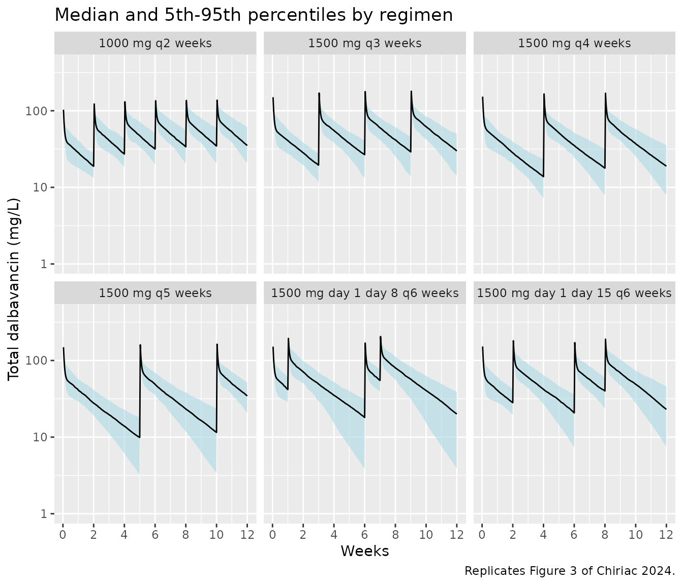
The PK/PD index is the free AUC over the last 24 h before redosing (Methods 4.3). The AUC is taken here before the last redose inside the 12-week window (week 12, or week 10 for the 5-week interval) and computed with PKNCA.
win <- sim_reg |>
  dplyr::filter(time >= window_end - 24, time <= window_end, !is.na(Cc)) |>
  dplyr::select(regimen, id, time, Cc)

dose_reg <- dplyr::bind_rows(lapply(names(regimens), function(nm) {
  tidyr::expand_grid(id = seq_len(200L), time = regimens[[nm]]$doses) |>
    dplyr::mutate(regimen = nm, amt = regimens[[nm]]$amt)
}))
dose_reg$regimen <- factor(dose_reg$regimen, levels = names(regimens))

intervals_reg <- tibble::tibble(
  regimen = factor(names(regimens), levels = names(regimens)),
  start = vapply(regimens, function(r) r$end - 24, numeric(1)),
  end = vapply(regimens, function(r) r$end, numeric(1)),
  auclast = TRUE
)

nca_reg <- PKNCA::pk.nca(PKNCA::PKNCAdata(
  PKNCA::PKNCAconc(win, Cc ~ time | regimen + id),
  PKNCA::PKNCAdose(dose_reg, amt ~ time | regimen + id),
  intervals = intervals_reg
))
auc_reg <- as.data.frame(nca_reg) |>
  dplyr::filter(PPTESTCD == "auclast") |>
  dplyr::select(regimen, id, auc24 = PPORRES)
stopifnot(nrow(auc_reg) == 6L * 200L, !anyNA(auc_reg$auc24))

mics <- c(0.016, 0.032, 0.064, 0.125, 0.25, 0.5, 1, 2)
pta <- tidyr::expand_grid(auc_reg, pb = 93:99, mic = mics) |>
  dplyr::group_by(regimen, pb, mic) |>
  dplyr::summarise(pta = 100 * mean(auc24 * (1 - pb / 100) / mic > 27.1), .groups = "drop")
ggplot(pta, aes(factor(mic), pta, colour = factor(pb), group = factor(pb))) +
  geom_line() +
  geom_point(shape = 15) +
  facet_wrap(~regimen, ncol = 3) +
  labs(
    x = "MIC (mg/L)", y = "PTA fAUC24h/MIC > 27.1 (%)", colour = "PB (%)",
    title = "Probability of target attainment for stasis",
    caption = "Replicates Figure 4 of Chiriac 2024."
  ) +
  theme(axis.text.x = element_text(angle = 45, hjust = 1))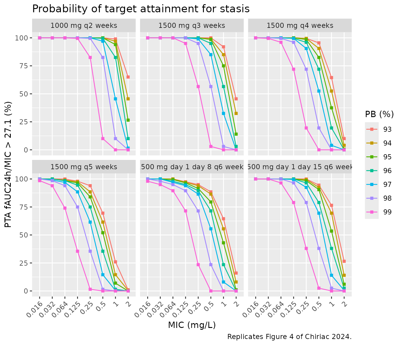
The PTA values below were digitised by the maintainers from Figure 4 at the two extreme protein-binding scenarios, on the steep part of each curve where the comparison is informative.
fig4 <- tibble::tribble(
  ~regimen,                         ~pb, ~mic,  ~pta_paper,
  "1000 mg q2 weeks",               99,  0.25,  85,
  "1000 mg q2 weeks",               99,  0.5,   12,
  "1000 mg q2 weeks",               93,  2,     75,
  "1500 mg q3 weeks",               99,  0.125, 96,
  "1500 mg q3 weeks",               99,  0.25,  66,
  "1500 mg q3 weeks",               93,  1,     94,
  "1500 mg q3 weeks",               93,  2,     53,
  "1500 mg q4 weeks",               99,  0.125, 76,
  "1500 mg q4 weeks",               99,  0.25,  21,
  "1500 mg q4 weeks",               93,  1,     68,
  "1500 mg q4 weeks",               93,  2,     12,
  "1500 mg q5 weeks",               99,  0.064, 82,
  "1500 mg q5 weeks",               99,  0.125, 45,
  "1500 mg q5 weeks",               93,  0.5,   78,
  "1500 mg q5 weeks",               93,  1,     35,
  "1500 mg day 1 day 8 q6 weeks",   99,  0.064, 92,
  "1500 mg day 1 day 8 q6 weeks",   99,  0.125, 73,
  "1500 mg day 1 day 8 q6 weeks",   99,  0.25,  28,
  "1500 mg day 1 day 8 q6 weeks",   93,  1,     67,
  "1500 mg day 1 day 8 q6 weeks",   93,  2,     20,
  "1500 mg day 1 day 15 q6 weeks",  99,  0.125, 86,
  "1500 mg day 1 day 15 q6 weeks",  99,  0.25,  43,
  "1500 mg day 1 day 15 q6 weeks",  93,  1,     81,
  "1500 mg day 1 day 15 q6 weeks",  93,  2,     32
)
fig4_cmp <- fig4 |>
  dplyr::mutate(regimen = factor(regimen, levels = names(regimens))) |>
  dplyr::inner_join(pta, by = c("regimen", "pb", "mic")) |>
  dplyr::mutate(diff = pta - pta_paper)
stopifnot(nrow(fig4_cmp) == nrow(fig4))

fig4_cmp |>
  dplyr::rename(
    "Regimen" = regimen, "PB (%)" = pb, "MIC (mg/L)" = mic,
    "PTA, Figure 4 (%)" = pta_paper, "PTA, model (%)" = pta,
    "Difference (points)" = diff
  ) |>
knitr::kable(digits = c(0, 0, 3, 0, 0, 0), caption = "PTA for stasis: digitised Figure 4 vs. 200 simulated patients per regimen.")| Regimen | PB (%) | MIC (mg/L) | PTA, Figure 4 (%) | PTA, model (%) | Difference (points) |
|---|---|---|---|---|---|
| 1000 mg q2 weeks | 99 | 0.250 | 85 | 82 | -2 |
| 1000 mg q2 weeks | 99 | 0.500 | 12 | 10 | -2 |
| 1000 mg q2 weeks | 93 | 2.000 | 75 | 65 | -10 |
| 1500 mg q3 weeks | 99 | 0.125 | 96 | 95 | -1 |
| 1500 mg q3 weeks | 99 | 0.250 | 66 | 56 | -10 |
| 1500 mg q3 weeks | 93 | 1.000 | 94 | 92 | -2 |
| 1500 mg q3 weeks | 93 | 2.000 | 53 | 46 | -8 |
| 1500 mg q4 weeks | 99 | 0.125 | 76 | 72 | -4 |
| 1500 mg q4 weeks | 99 | 0.250 | 21 | 20 | -2 |
| 1500 mg q4 weeks | 93 | 1.000 | 68 | 64 | -4 |
| 1500 mg q4 weeks | 93 | 2.000 | 12 | 10 | -2 |
| 1500 mg q5 weeks | 99 | 0.064 | 82 | 74 | -8 |
| 1500 mg q5 weeks | 99 | 0.125 | 45 | 36 | -10 |
| 1500 mg q5 weeks | 93 | 0.500 | 78 | 70 | -8 |
| 1500 mg q5 weeks | 93 | 1.000 | 35 | 26 | -9 |
| 1500 mg day 1 day 8 q6 weeks | 99 | 0.064 | 92 | 90 | -2 |
| 1500 mg day 1 day 8 q6 weeks | 99 | 0.125 | 73 | 72 | -2 |
| 1500 mg day 1 day 8 q6 weeks | 99 | 0.250 | 28 | 24 | -4 |
| 1500 mg day 1 day 8 q6 weeks | 93 | 1.000 | 67 | 64 | -2 |
| 1500 mg day 1 day 8 q6 weeks | 93 | 2.000 | 20 | 16 | -4 |
| 1500 mg day 1 day 15 q6 weeks | 99 | 0.125 | 86 | 79 | -7 |
| 1500 mg day 1 day 15 q6 weeks | 99 | 0.250 | 43 | 38 | -5 |
| 1500 mg day 1 day 15 q6 weeks | 93 | 1.000 | 81 | 76 | -4 |
| 1500 mg day 1 day 15 q6 weeks | 93 | 2.000 | 32 | 26 | -6 |
# A PTA from 200 patients has a binomial SE of up to 3.5 points, the
# digitisation about 2 points; a 20% error in CL or V shifts the steep part of
# these curves by 20-40 points. Centre and robust envelope, not the worst row.
stopifnot(
  median(abs(fig4_cmp$diff)) < 8,
  quantile(abs(fig4_cmp$diff), 0.9) < 20
)

# Results 2.3: at 99% protein binding and the 0.125 mg/L ECOFF, only 1000 mg
# q2 weeks and 1500 mg q3 weeks reach PTA >= 90%. The two passing regimens sit
# at about 95-100% and the best failing one near 80%, each several binomial SEs
# from the 90% line.
pta_ecoff <- pta |> dplyr::filter(pb == 99, mic == 0.125)
stopifnot(nrow(pta_ecoff) == 6L)
passing <- as.character(pta_ecoff$regimen[pta_ecoff$pta >= 90])
stopifnot(setequal(passing, c("1000 mg q2 weeks", "1500 mg q3 weeks")))
The simulated curves follow Figure 4, and the paper’s headline result is reproduced: at 99% protein binding and an MIC of 0.125 mg/L only 1000 mg every 2 weeks and 1500 mg every 3 weeks keep the PTA at or above 90% (Results 2.3). The simulated PTA sits 1-10 points below the digitised values throughout, most for the 5-week interval. That regimen has only one complete interval before its week-10 redose; when the same calculation is moved to later intervals of a longer dose train, its PTA at 99% binding and 0.125 mg/L rises from about 37% towards 42%, closer to the figure’s 45%. The paper’s PTA was therefore probably evaluated nearer steady state than the 12 weeks plotted in Figure 3, which the paper does not state.
Assumptions and deviations
- Infusion duration. Not reported; the 30-minute infusion of the product label is assumed. It affects only the first hour after each dose.
- Monolix omega scale. Table 2 reports omega for CL, V1 and V2 as Monolix does, as the standard deviation of the log-normal random effect; the packaged variances are omega squared.
-
Fixed Q. Q = 0.476 L/h is fixed in the source
(Results 2.2, Table 2 with no RSE) to the value of Buckwalter 2005 and
is encoded with
fixed(). No IIV on Q is reported. - Albumin unit. Table 1 prints albumin as 42.5 +/- 5.7 ‘mg/dL’; the value is physiologically g/L. Albumin was not retained in the model.
- Table S5 redose. Table S5 does not say before which redose its AUC24h was taken; the AUC before the third 6-week cycle reproduces all 13 rows within 1.5%, so that reading is used. One patient received 1000 mg instead of 1500 mg (Results 2.1) but is not identified; every patient is simulated at 1500 mg, and all 13 rows still agree.
- PTA window. The AUC window for Figure 4 is taken before the last redose inside the 12-week window of Figure 3. The paper does not state the simulation horizon for the PTA; see the comment under the Figure 4 comparison.
- Figure 5 (cumulative fraction of response). Not replicated: it weights the PTA curves by the EUCAST S. aureus dalbavancin MIC distribution, which the paper cites but does not print.
- Week-6 trough. The simulated mean week-6 concentration exceeds the observed mean of 13.2 mg/L; the observed value is depressed by the half-quantification-limit imputation of below-limit samples (Methods 4.2).
- No erratum or correction notice was found for this article (EuropePMC search, 2026-10-31).