Teclistamab bell-shaped trimer QSP (Gevertz 2025)
Source:vignettes/articles/Gevertz_2025_teclistamab.Rmd
Gevertz_2025_teclistamab.RmdModel and source
- Citation: Gevertz JL, Kareva I. Using Virtual Patients to Evaluate Dosing Strategies for Bispecifics With a Bell-Shaped Efficacy Curve. CPT Pharmacometrics Syst Pharmacol. 2025;14(12):2139-2148. doi:10.1002/psp4.70105. Model equations (1)-(18) and Table S1 are in Supporting Information Data S1; the authors’ MATLAB implementation is at https://github.com/jgevertz/teclistamab (commit e6dc5479). The time-varying clearance component and the 74 kg reference weight come from Miao et al. (2023) Target Oncol 18:667-684 (reference 5 of Data S1), see modellib(‘Miao_2023_teclistamab’).
- Description: QSP. Semi-mechanistic PK/PD model of teclistamab, a
BCMA x CD3 bispecific T-cell engager, in relapsed/refractory multiple
myeloma, built to locate the peak of the bell-shaped trimer-versus-dose
curve. Free drug follows two-compartment disposition with first-order
subcutaneous absorption and a clearance that decays exponentially from
the first dose, and distributes into a bone-marrow (tumour
microenvironment) compartment. Drug binds CD3 (on T cells, produced in a
thymus compartment) and soluble BCMA in plasma, and CD3, soluble BCMA
and membrane-bound BCMA in bone marrow, by mass action, forming dimers
and trimers. Only the bone-marrow drug-CD3-membrane BCMA trimer
(
trimer, the pharmacologically active trimer, PAT) is efficacious. The initial conditions are the authors’ pre-equilibration starting values, not the drug-free steady state: the authors run the model drug-free for 50 days before the first dose, so dose at day 50 to reproduce the published simulations. Inter-individual variability on the five virtual-patient attributes (Cl1, kshed, baseline membrane BCMA, k1bm and baseline bone-marrow CD3) reproduces the paper’s virtual population. Parameter values and equations are the published Table S1 and Eqs (1)-(18). The published figures were produced by the authors’ code, which uses a lower membrane BCMA internalisation rate (0.554/day, not 2/day) and CD3 internalisation rate (1.584/day, not 16.6/day) among other differences; with the Table S1 values the median PAT peak of the virtual population moves from about 1.5-1.8 mg/kg to about 5 mg/kg weekly. The validation article rebuilds the code configuration and reproduces the paper’s 1.8 mg/kg Q1W and 3 mg/kg Q2W optima. - Article: https://doi.org/10.1002/psp4.70105
- Model equations and parameter table: Supporting Information Data S1 of the article.
- Authors’ MATLAB code: https://github.com/jgevertz/teclistamab (commit
e6dc5479).
Gevertz and Kareva build a semi-mechanistic PK/PD model of teclistamab, a BCMA x CD3 bispecific T-cell engager, to ask which dose maximises the pharmacologically active trimer (PAT: drug + CD3 + membrane BCMA in the bone marrow). Because only the trimer is active, the PAT-versus-dose curve is bell-shaped: too little drug forms few trimers, and too much drug saturates CD3 and BCMA separately as dimers. The paper finds the median normalised PAT AUC over 1200 virtual patients peaks at 1.8 mg/kg for weekly (Q1W) and 3 mg/kg for every-two-weeks (Q2W) subcutaneous dosing, close to the approved 1.5 mg/kg Q1W regimen.
Population
No model was fitted to patient-level data. The PK backbone comes from
the MajesTEC-1 population PK analysis (Miao 2023, see
modellib("Miao_2023_teclistamab")) and from Girgis 2022,
whose mean plasma PK at 0.72 and 1.5 mg/kg SC is reproduced in Figure
2A. Target-binding and turnover parameters are literature values (Table
S1). The virtual population is 1200 patients with relapsed/refractory
multiple myeloma, each defined by independent lognormal draws of five
attributes (Figure S2): the time-independent clearance Cl1, the BCMA
shedding rate kshed, the baseline membrane BCMA in the bone marrow, the
plasma-to-bone-marrow drug distribution rate k1bm, and the baseline
bone-marrow CD3.
readModelDb("Gevertz_2025_teclistamab_qsp")()$population
#> $species
#> [1] "human"
#>
#> $n_subjects
#> [1] NA
#>
#> $disease_state
#> [1] "relapsed/refractory multiple myeloma (virtual patients)"
#>
#> $dose_range
#> [1] "0.1-10 mg/kg SC Q1W or Q2W after step-up doses of 0.06 and 0.3 mg/kg one week apart (Figure 5); 0.72 and 1.5 mg/kg SC Q1W for the PK benchmark (Figure 2)"
#>
#> $notes
#> [1] "No model was fitted to subject-level data. Structural PK values are taken or derived from the MajesTEC-1 population PK analysis (Miao 2023) and from Girgis 2022, whose digitised mean plasma PK at 0.72 and 1.5 mg/kg SC is reproduced in Figure 2A; target-binding and turnover values are from the literature cited in Table S1. The virtual population is 1200 virtual patients, each defined by independent lognormal draws of Cl1, kshed, baseline membrane BCMA in bone marrow, k1bm and baseline bone-marrow CD3 (Figure S2), chosen to mimic the size of a Phase 3 trial."
Source trace
All equations are Supporting Information Data S1 Eqs (1)-(18); all
values are Table S1 of Data S1 unless stated. The in-file comments in
inst/modeldb/specificDrugs/Gevertz_2025_teclistamab_qsp.R
give the same information line by line.
| Model element | Value | Source |
|---|---|---|
d/dt(depot), d/dt(central),
d/dt(peripheral1)
|
– | Eqs (4), (5), (6) |
d/dt(target_cd3_thymus),
d/dt(target_cd3_central), d/dt(target)
|
– | Eqs (1), (2), (3) |
d/dt(complex), d/dt(drug_cd3_central),
d/dt(complex_cd3_sbcma)
|
– | Eqs (7), (8), (9) |
d/dt(target_bcma_bonemarrow),
d/dt(target_bonemarrow),
d/dt(target_cd3_bonemarrow)
|
– | Eqs (10), (11), (12) |
d/dt(bonemarrow) |
– | Eq (13) |
d/dt(drug_cd3_bonemarrow),
d/dt(complex_bonemarrow),
d/dt(drug_bcma_bonemarrow)
|
– | Eqs (14), (15), (16) |
d/dt(complex_cd3_sbcma_bonemarrow),
d/dt(trimer)
|
– | Eqs (17), (18) |
Synthesis rates ksyn = baseline x loss rate
|
– | Data S1 text after Eq (13); Table S1 kth1 for the thymus |
cl = Cl1 + Clvar exp(-delta t) |
– | Table S1 Cl1 row; form as coded by the authors |
lka (k01) |
0.2 1/day | Table S1 |
lvc (V1) |
3 L | Table S1 ‘3-4 L’; k10 = Cl1/V1 = 0.17 and k12 = Cl2/V1 = 0.13 both give 3 L |
lvp (V2) |
1.34 L | Table S1 |
lq (Cl2) |
0.4 L/day | Table S1 |
lcl_exp_inf (Cl1) |
0.5 L/day | Table S1 |
lcl_exp_component (Clvar) |
0.547 L/day | Table S1 cites ref 5 (Miao 2023 Table 2, CL2) |
lcl_exp_kdes (delta) |
0.1 1/day | Table S1 |
vbm (Vbm) |
2.2 L | Table S1 |
lktr_ab_c_bm (k1bm), ktr_ab_bm_c
(kbm1) |
0.1, 0.001 1/day | Table S1 |
kon_cd3, koff_cd3
|
10 1/nM/day, 285 1/day | Table S1 kon3,p, koff3,p |
kon_sbcma, koff_sbcma
|
111 1/nM/day, 20 1/day | Table S1 kon,sB, koff,sB |
kon_mbcma, koff_mbcma
|
111 1/nM/day, 20 1/day | Table S1 kon,mB, koff,mB |
ktr_cd3_thymus_c (kth1) |
0.5 1/day | Table S1 |
kint_cd3 (kint3) |
16.6 1/day | Table S1 |
ktr_cd3_bm_c, ktr_cd3_c_bm (k3,bm1,
k3,1bm) |
0.1, 0.01 1/day | Table S1 |
lkshed (kshed) |
0.05 1/day | Table S1 |
kint_bcma (kint,mB) |
2 1/day | Table S1 |
kdeg_sbcma (k10,sB) |
0.04 1/day | Table S1 |
ktr_sbcma_bm_c, ktr_sbcma_c_bm (kB,bm1,
kB,1bm) |
0.1, 0.1 1/day | Table S1 |
kel_complex_bm (kout) |
0.01 1/day | Table S1 |
bl_cd3_thymus, bl_cd3_central,
lbl_cd3_bm
|
0.001, 0.01, 0.1 nM | Table S1 nonzero initial conditions |
bl_sbcma, lbl_mbcma_bm,
bl_sbcma_bm
|
20, 50, 3 nM | Table S1 nonzero initial conditions |
etalcl_exp_inf |
0.518 | Figure S2A, mean 6.0676, SD 5 (mL/kg/day) |
etalkshed |
1.085 | Figure S2B, mean 0.05, SD 0.07 |
etalbl_mbcma_bm |
0.148 | Figure S2C, mean 50, SD 20 |
etalktr_ab_c_bm |
0.0392 | Figure S2D, mean 0.1, SD 0.02 |
etalbl_cd3_bm |
0.00995 | Figure S2E, mean 0.1, SD 0.01 |
Each variance is log(1 + (SD / mean)^2), the log-scale
variance of a lognormal distribution with that arithmetic mean and
SD.
Dosing helpers
Doses are in mg/kg in the paper. Teclistamab is 146 kDa (Methods), so
1 mg is 6.849 nmol, and a mg/kg dose is converted at the 74 kg reference
weight that the authors’ code uses. Every regimen starts with step-up
doses of 0.06 and 0.3 mg/kg one week apart, followed by ten treatment
doses Q1W or Q2W from day 14. The authors run the model drug-free for 50
days before the first dose, so here the first dose is at model time 50
and results are reported against time since the first dose,
t = time - 50.
mw_kda <- 146
ref_wt <- 74
t_eq <- 50
mgkg_to_nmol <- function(mgkg) mgkg * ref_wt * 1e6 / (mw_kda * 1000)

# Simulation horizon used by the authors: all doses plus one more interval
horizon <- function(freq_wk) 14 + 7 * freq_wk * 11

make_regimen <- function(id, dose, freq_wk, dt_obs = 0.5) {
  ii <- 7 * freq_wk
  doses <- data.frame(
    id = id, time = t_eq + c(0, 7, 14 + ii * (0:9)),
    amt = mgkg_to_nmol(c(0.06, 0.3, rep(dose, 10))), evid = 1L, cmt = "depot"
  )
  obs <- data.frame(
    id = id, time = t_eq + seq(0, horizon(freq_wk), by = dt_obs),
    amt = NA_real_, evid = 0L, cmt = "central"
  )
  bind_rows(doses, obs)
}
Model as published
The packaged model uses the Table S1 values and the printed Eqs (1)-(18). Figure 2 of the paper plots free plasma drug (in ng/mL) and the PAT for the 0.72 and 1.5 mg/kg SC Q1W regimens at the nominal parameter values.
mod <- readModelDb("Gevertz_2025_teclistamab_qsp")
mod_typ <- rxode2::zeroRe(mod)
#> ℹ parameter labels from comments will be replaced by 'label()'

# With the random effects zeroed, rxode2 notes that a multi-subject solve has
# no omega; that is intended here (typical values, or etas supplied per
# patient), so only that one message is muffled.
solve_quiet <- function(...) {
  withCallingHandlers(
    rxode2::rxSolve(..., returnType = "data.frame"),
    warning = function(w) {
      if (grepl("without 'omega'", conditionMessage(w), fixed = TRUE)) invokeRestart("muffleWarning")
    }
  )
}

ev_fig2 <- bind_rows(
  make_regimen(1, 0.72, 1, dt_obs = 0.1),
  make_regimen(2, 1.5, 1, dt_obs = 0.1)
) |>
  filter(time <= t_eq + 80)
lab_fig2 <- c(`1` = "0.72 mg/kg SC Q1W", `2` = "1.5 mg/kg SC Q1W")

sim_pub <- solve_quiet(mod_typ, ev_fig2) |>
  mutate(t = time - t_eq, regimen = lab_fig2[as.character(id)], config = "Table S1 (packaged)")
#> ℹ omega/sigma items treated as zero: 'etalcl_exp_inf', 'etalkshed', 'etalbl_mbcma_bm', 'etalktr_ab_c_bm', 'etalbl_cd3_bm'
Authors’ code configuration
The published figures were produced by the authors’ MATLAB code,
which differs from Table S1 and the printed equations in the places
listed under “Assumptions and deviations”. The block below rebuilds that
configuration from the packaged model with ini() and
model() overrides, so the figures can be compared
directly.
mod_code <- mod |>
  rxode2::ini(
    lcl_exp_inf = log(0.449),
    kint_cd3 = 1.584,
    kint_bcma = 0.693 / 1.25,
    kon_cd3 = 285 / 28.03,
    kon_sbcma = 20 / 0.18,
    kon_mbcma = 20 / 0.18
  ) |>
  rxode2::model({
    # Drug-sBCMA complexes in plasma cleared at the drug elimination rate k10
    d/dt(complex) <- kon_sbcma * target * central - koff_sbcma * complex -
      kon_cd3 * target_cd3_central * complex + koff_cd3 * complex_cd3_sbcma - kel * complex
    d/dt(complex_cd3_sbcma) <- kon_sbcma * target * drug_cd3_central - koff_sbcma * complex_cd3_sbcma +
      kon_cd3 * target_cd3_central * complex - koff_cd3 * complex_cd3_sbcma -
      kint_cd3 * complex_cd3_sbcma - kel * complex_cd3_sbcma
    # sBCMA enters the marrow at the drug rate k1bm with the V1/Vbm volume ratio
    d/dt(target_bonemarrow) <- kshed * target_bcma_bonemarrow - ktr_sbcma_bm_c * target_bonemarrow -
      kon_sbcma * target_bonemarrow * bonemarrow + koff_sbcma * complex_bonemarrow -
      kon_sbcma * target_bonemarrow * drug_cd3_bonemarrow + koff_sbcma * complex_cd3_sbcma_bonemarrow +
      vc / vbm * ktr_ab_c_bm * target
    # Bone-marrow drug-sBCMA dimer cleared at kout
    d/dt(complex_bonemarrow) <- kon_sbcma * target_bonemarrow * bonemarrow - koff_sbcma * complex_bonemarrow -
      kon_cd3 * target_cd3_bonemarrow * complex_bonemarrow + koff_cd3 * complex_cd3_sbcma_bonemarrow -
      kel_complex_bm * complex_bonemarrow
  })
#> ℹ parameter labels from comments will be replaced by 'label()'
#> ℹ change initial estimate of `lcl_exp_inf` to `-0.800732391239883`
#> ℹ change initial estimate of `kint_cd3` to `1.584`
#> ℹ change initial estimate of `kint_bcma` to `0.5544`
#> ℹ change initial estimate of `kon_cd3` to `10.1676774884053`
#> ℹ change initial estimate of `kon_sbcma` to `111.111111111111`
#> ℹ change initial estimate of `kon_mbcma` to `111.111111111111`
mod_code_typ <- rxode2::zeroRe(mod_code)

sim_code <- solve_quiet(mod_code_typ, ev_fig2) |>
  mutate(t = time - t_eq, regimen = lab_fig2[as.character(id)], config = "Authors' code")
#> ℹ omega/sigma items treated as zero: 'etalcl_exp_inf', 'etalkshed', 'etalbl_mbcma_bm', 'etalktr_ab_c_bm', 'etalbl_cd3_bm'
Figure 2A: plasma PK
The points are the Girgis 2022 mean plasma concentrations as
digitised by the authors and stored in their code
(trimer_teclistimab_vs_data.m), shifted by 14 days to the
start of treatment dosing.
girgis <- data.frame(
  regimen = rep(c("0.72 mg/kg SC Q1W", "1.5 mg/kg SC Q1W"), c(7, 6)),
  t = c(c(0, 0.1, 1, 2, 3, 5, 7), c(0, 0.1, 1, 2, 3, 7)) + 14,
  conc = c(
    1252.630175, 1326.291716, 3118.900845, 4159.151398, 4951.204559, 3977.371187, 4621.028168,
    1571.719325, 1712.376561, 5347.643161, 7335.807348, 8488.477506, 7923.179002
  )
)

fig2 <- bind_rows(sim_pub, sim_code)

ggplot(filter(fig2, t > 0, Cc * mw_kda >= 10), aes(t, Cc * mw_kda, colour = regimen, linetype = config)) +
  geom_line() +
  geom_point(data = girgis, aes(t, conc, colour = regimen), inherit.aes = FALSE) +
  geom_hline(yintercept = c(369, 2272, 6028), linetype = "dotted") +
  scale_y_log10() +
  labs(
    x = "Time since first step-up dose (day)", y = "Free plasma teclistamab (ng/mL)",
    colour = NULL, linetype = NULL,
    caption = "Replicates Figure 2A of Gevertz 2025. Dotted lines: EC50, EC90 and max EC90."
  )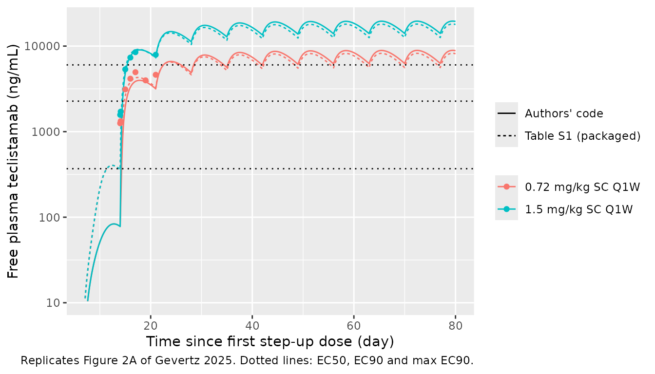
Figure 2B: pharmacologically active trimer
ggplot(filter(fig2, t > 0, trimer >= 1e-3), aes(t, trimer, colour = regimen, linetype = config)) +
  geom_line() +
  scale_y_log10() +
  labs(
    x = "Time since first step-up dose (day)", y = "PAT in bone marrow (nM)",
    colour = NULL, linetype = NULL,
    caption = "Replicates Figure 2B of Gevertz 2025."
  )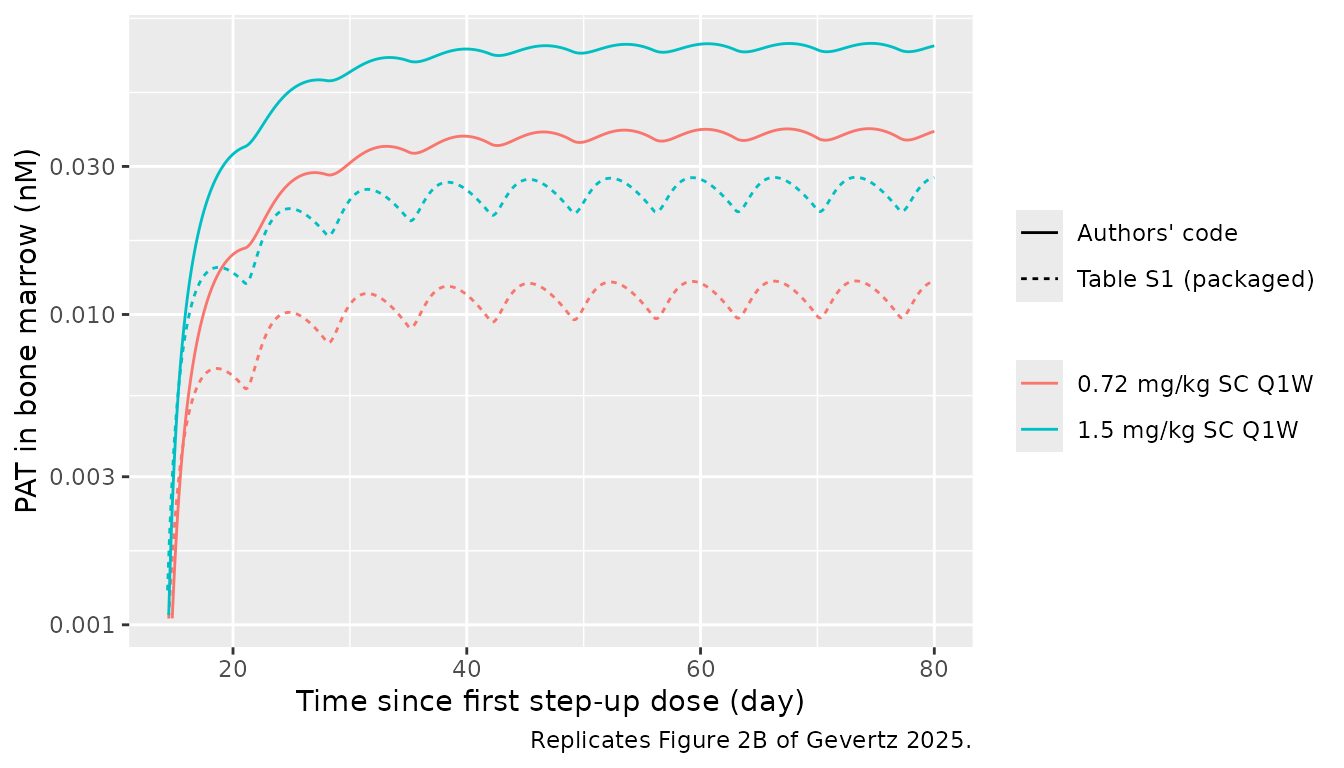
Figure 2B shows the PAT reaching about 0.04 nM at 0.72 mg/kg and 0.07 nM at 1.5 mg/kg by day 80. The authors’ code configuration reproduces this. The Table S1 values give a PAT about 3.5 times lower, because membrane BCMA (and with it the PAT) is internalised at 2/day rather than 0.554/day.
fig2_ss <- fig2 |>
  filter(abs(t - 77) < 1e-6) |>
  select(config, regimen, Cc, trimer) |>
  mutate(Cc_ngml = Cc * mw_kda)
fig2_ss |>
  select(config, regimen, Cc_ngml, trimer) |>
  rename(
    Configuration = config, Regimen = regimen,
    "Free plasma drug at day 77 (ng/mL)" = Cc_ngml, "PAT at day 77 (nM)" = trimer
  ) |>
knitr::kable(digits = c(0, 0, 0, 4))| Configuration | Regimen | Free plasma drug at day 77 (ng/mL) | PAT at day 77 (nM) |
|---|---|---|---|
| Table S1 (packaged) | 0.72 mg/kg SC Q1W | 5603 | 0.0099 |
| Table S1 (packaged) | 1.5 mg/kg SC Q1W | 12587 | 0.0217 |
| Authors’ code | 0.72 mg/kg SC Q1W | 6259 | 0.0371 |
| Authors’ code | 1.5 mg/kg SC Q1W | 14048 | 0.0713 |
pat_code <- setNames(fig2_ss$trimer[fig2_ss$config == "Authors' code"],
                     fig2_ss$regimen[fig2_ss$config == "Authors' code"])
stopifnot(
  # Figure 2B plateaus, read off the published log axis
  abs(pat_code[["0.72 mg/kg SC Q1W"]] / 0.04 - 1) < 0.15,
  abs(pat_code[["1.5 mg/kg SC Q1W"]] / 0.07 - 1) < 0.15
)
The 1.5 mg/kg data are tracked closely. The day-14 points sit above both curves, as they do in the published Figure 2A, because they are pre-dose values from a study without the step-up schedule.
Virtual population
Each virtual patient draws its five attributes independently from
lognormal distributions whose arithmetic mean is the nominal value and
whose SD is given in Figure S2. The model’s random effects are centred
so that the nominal value is the median; to reproduce the paper’s
mean-preserving draws, each eta is sampled here from
N(-omega^2 / 2, omega^2) and passed to
rxSolve() as a fixed per-patient value. The authors’ code
centres Cl1 on 0.449 L/day (Figure S2A mean 6.0676 mL/kg/day at 74 kg),
which is the value the code configuration uses.
n_vp <- 100
omega <- c(
  etalcl_exp_inf = 0.518232, etalkshed = 1.085189, etalbl_mbcma_bm = 0.148420,
  etalktr_ab_c_bm = 0.039221, etalbl_cd3_bm = 0.009950
)
set.seed(20251)
vp_eta <- as.data.frame(lapply(omega, function(w) rnorm(n_vp, -w / 2, sqrt(w))))
vp_eta$vp <- seq_len(n_vp)

# Arithmetic means of the sampled attributes against Figure S2
vp_check <- data.frame(
  attribute = c("Cl1 (mL/kg/day)", "kshed (1/day)", "mBbm0 (nM)", "k1bm (1/day)", "CD3bm0 (nM)"),
  paper_mean = c(6.0676, 0.05, 50, 0.1, 0.1),
  paper_sd = c(5, 0.07, 20, 0.02, 0.01)
)
vp_values <- cbind(
  0.449 * 1000 / ref_wt * exp(vp_eta$etalcl_exp_inf),
  0.05 * exp(vp_eta$etalkshed),
  50 * exp(vp_eta$etalbl_mbcma_bm),
  0.1 * exp(vp_eta$etalktr_ab_c_bm),
  0.1 * exp(vp_eta$etalbl_cd3_bm)
)
vp_check$sample_mean <- colMeans(vp_values)
vp_check$sample_sd <- apply(vp_values, 2, sd)
vp_check |>
  rename(
    Attribute = attribute, "Figure S2 mean" = paper_mean, "Figure S2 SD" = paper_sd,
    "Sampled mean" = sample_mean, "Sampled SD" = sample_sd
  ) |>
knitr::kable(digits = 4)| Attribute | Figure S2 mean | Figure S2 SD | Sampled mean | Sampled SD |
|---|---|---|---|---|
| Cl1 (mL/kg/day) | 6.0676 | 5.00 | 6.1506 | 4.9751 |
| kshed (1/day) | 0.0500 | 0.07 | 0.0510 | 0.0537 |
| mBbm0 (nM) | 50.0000 | 20.00 | 45.9601 | 16.1925 |
| k1bm (1/day) | 0.1000 | 0.02 | 0.1011 | 0.0177 |
| CD3bm0 (nM) | 0.1000 | 0.01 | 0.0995 | 0.0104 |
With 100 draws the sampled kshed SD is noisy (its CV is 140%), but the means agree with Figure S2.
Figure 5: dose sweep
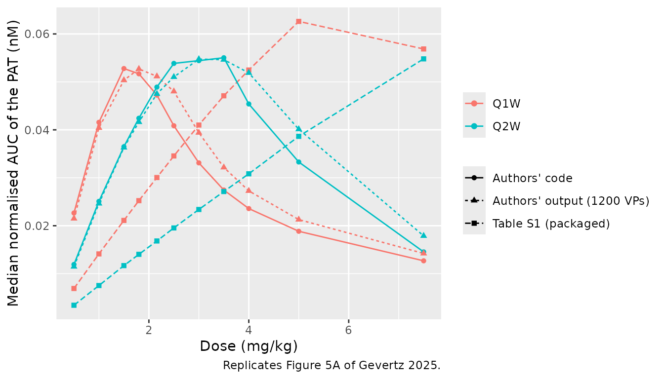
The paper sweeps 20 doses from 0.1 to 10 mg/kg for Q1W and Q2W and reports the median, over virtual patients, of the PAT AUC over the whole simulation (all doses plus one interval), divided by the simulation length. A subset of 11 doses around the peak is simulated here for each schedule. Each dose x schedule arm is the same 100 virtual patients.
doses <- c(0.5, 1, 1.5, 1.8, 2.16, 2.5, 3, 3.5, 4, 5, 7.5)
arms <- expand.grid(vp = seq_len(n_vp), dose = doses, freq_wk = 1:2)
arms$id <- seq_len(nrow(arms))
arms$arm <- sprintf("%s mg/kg Q%dW", arms$dose, arms$freq_wk)

ev_sweep <- bind_rows(Map(make_regimen, arms$id, arms$dose, arms$freq_wk)) |>
  arrange(id, time, desc(evid))
params_sweep <- arms |>
  left_join(vp_eta, by = "vp") |>
  select(id, all_of(names(omega)))

solve_sweep <- function(m) {
  solve_quiet(m, ev_sweep, params = params_sweep) |>
    select(id, time, Cc, trimer, target, target_bcma_bonemarrow,
           drug_cd3_bonemarrow, complex_bonemarrow, drug_bcma_bonemarrow,
           complex_cd3_sbcma_bonemarrow) |>
    left_join(arms, by = "id") |>
    mutate(t = time - t_eq)
}
sweep_code <- solve_sweep(mod_code_typ)
sweep_pub <- solve_sweep(mod_typ)
PKNCA: AUC of the PAT
The PAT AUC is computed with PKNCA over [0, horizon]
with the linear trapezoidal rule, as the authors’ MATLAB
trapz() does. Small negative solver undershoots are set to
zero first, as the authors’ code also does.
pat_auc <- function(sw) {
  conc <- sw |>
    filter(!is.na(trimer)) |>
    mutate(trimer = pmax(trimer, 0)) |>
    select(id, arm, freq_wk, dose, t, trimer)
  intervals <- data.frame(
    freq_wk = 1:2, start = 0, end = horizon(1:2), auclast = TRUE
  )
  conc_obj <- PKNCA::PKNCAconc(conc, trimer ~ t | freq_wk + dose + arm + id)
  dat <- PKNCA::PKNCAdata(conc_obj, intervals = intervals,
                          options = list(auc.method = "linear"))
  PKNCA::pk.nca(dat)
}
nca_code <- pat_auc(sweep_code)
#> No dose information provided, calculations requiring dose will return NA.
nca_pub <- pat_auc(sweep_pub)
#> No dose information provided, calculations requiring dose will return NA.
The authors’ deposited output file
(output_teclistamab_VCT_parallel.mat) stores the median
un-normalised PAT AUC over all 1200 virtual patients at every swept
dose. The values at the 11 doses simulated here are compared below;
normalised values are these divided by 91 days (Q1W) or 168 days
(Q2W).
ref_auc <- tibble::tribble(
  ~dose, ~q1w, ~q2w,
  0.5, 1.9561546, 1.9273954,
  1, 3.6769656, 4.1375960,
  1.5, 4.5818599, 6.0995342,
  1.8, 4.7958474, 6.9935881,
  2.16, 4.6553422, 7.9792257,
  2.5, 4.3696357, 8.5726394,
  3, 3.5857448, 9.1963168,
  3.5, 2.9269314, 9.1777850,
  4, 2.4814512, 8.7152296,
  5, 1.9366015, 6.7412843,
  7.5, 1.2939786, 3.0042709
) |>
  pivot_longer(c(q1w, q2w), names_to = "sched", values_to = "auclast") |>
  mutate(freq_wk = ifelse(sched == "q1w", 1L, 2L), arm = sprintf("%s mg/kg Q%dW", dose, freq_wk)) |>
  select(arm, auclast)

cmp <- nlmixr2lib::ncaComparisonTable(
  simulated = nca_code,
  reference = as.data.frame(ref_auc),
  by = "arm",
  params = "auclast",
  units = c(auclast = "nM*day"),
  tolerance_pct = 20
)
knitr::kable(
  cmp,
  caption = "Median PAT AUC, authors' code configuration (100 virtual patients) vs the authors' output file (1200 virtual patients). * differs by >20%."
)| NCA parameter | arm | Reference | Simulated | % diff |
|---|---|---|---|---|
| AUClast (nM*day) | 0.5 mg/kg Q1W | 1.96 | 2.06 | +5.4% |
| AUClast (nM*day) | 0.5 mg/kg Q2W | 1.93 | 2 | +3.9% |
| AUClast (nM*day) | 1 mg/kg Q1W | 3.68 | 3.78 | +2.9% |
| AUClast (nM*day) | 1 mg/kg Q2W | 4.14 | 4.21 | +1.8% |
| AUClast (nM*day) | 1.5 mg/kg Q1W | 4.58 | 4.8 | +4.8% |
| AUClast (nM*day) | 1.5 mg/kg Q2W | 6.1 | 6.13 | +0.5% |
| AUClast (nM*day) | 1.8 mg/kg Q1W | 4.8 | 4.7 | -1.9% |
| AUClast (nM*day) | 1.8 mg/kg Q2W | 6.99 | 7.13 | +1.9% |
| AUClast (nM*day) | 2.16 mg/kg Q1W | 4.66 | 4.3 | -7.6% |
| AUClast (nM*day) | 2.16 mg/kg Q2W | 7.98 | 8.22 | +3.0% |
| AUClast (nM*day) | 2.5 mg/kg Q1W | 4.37 | 3.72 | -14.9% |
| AUClast (nM*day) | 2.5 mg/kg Q2W | 8.57 | 9.05 | +5.5% |
| AUClast (nM*day) | 3 mg/kg Q1W | 3.59 | 3.01 | -16.0% |
| AUClast (nM*day) | 3 mg/kg Q2W | 9.2 | 9.14 | -0.6% |
| AUClast (nM*day) | 3.5 mg/kg Q1W | 2.93 | 2.5 | -14.7% |
| AUClast (nM*day) | 3.5 mg/kg Q2W | 9.18 | 9.25 | +0.7% |
| AUClast (nM*day) | 4 mg/kg Q1W | 2.48 | 2.15 | -13.5% |
| AUClast (nM*day) | 4 mg/kg Q2W | 8.72 | 7.63 | -12.5% |
| AUClast (nM*day) | 5 mg/kg Q1W | 1.94 | 1.71 | -11.4% |
| AUClast (nM*day) | 5 mg/kg Q2W | 6.74 | 5.59 | -17.0% |
| AUClast (nM*day) | 7.5 mg/kg Q1W | 1.29 | 1.15 | -10.8% |
| AUClast (nM*day) | 7.5 mg/kg Q2W | 3 | 2.44 | -18.7% |
med_auc <- function(nca, label) {
  as.data.frame(nca$result) |>
    filter(PPTESTCD == "auclast") |>
    group_by(freq_wk, dose) |>
    summarise(nauc = median(PPORRES) / horizon(freq_wk[1]), .groups = "drop") |>
    mutate(config = label)
}
fig5 <- bind_rows(
  med_auc(nca_code, "Authors' code"),
  med_auc(nca_pub, "Table S1 (packaged)"),
  ref_auc |>
    tidyr::separate(arm, c("dose", "x", "sched"), sep = " ", convert = TRUE) |>
    mutate(freq_wk = ifelse(sched == "Q1W", 1L, 2L), nauc = auclast / horizon(freq_wk),
           config = "Authors' output (1200 VPs)") |>
    select(freq_wk, dose, nauc, config)
) |>
  mutate(schedule = paste0("Q", freq_wk, "W"))

ggplot(fig5, aes(dose, nauc, colour = schedule, linetype = config, shape = config)) +
  geom_line() +
  geom_point() +
  labs(
    x = "Dose (mg/kg)", y = "Median normalised AUC of the PAT (nM)",
    colour = NULL, linetype = NULL, shape = NULL,
    caption = "Replicates Figure 5A of Gevertz 2025."
  )
optimum <- fig5 |>
  group_by(config, schedule) |>
  summarise(
    optimal_dose = dose[which.max(nauc)],
    near_optimal = paste(range(dose[nauc >= 0.9 * max(nauc)]), collapse = "-"),
    peak_nauc = max(nauc),
    .groups = "drop"
  )
optimum |>
  rename(
    Configuration = config, Schedule = schedule, "Optimal dose (mg/kg)" = optimal_dose,
    "Within 10% of peak (mg/kg)" = near_optimal, "Peak normalised AUC (nM)" = peak_nauc
  ) |>
knitr::kable(digits = 4)| Configuration | Schedule | Optimal dose (mg/kg) | Within 10% of peak (mg/kg) | Peak normalised AUC (nM) |
|---|---|---|---|---|
| Authors’ code | Q1W | 1.5 | 1.5-1.8 | 0.0528 |
| Authors’ code | Q2W | 3.5 | 2.5-3.5 | 0.0550 |
| Authors’ output (1200 VPs) | Q1W | 1.8 | 1.5-2.5 | 0.0527 |
| Authors’ output (1200 VPs) | Q2W | 3.0 | 2.5-4 | 0.0547 |
| Table S1 (packaged) | Q1W | 5.0 | 5-7.5 | 0.0626 |
| Table S1 (packaged) | Q2W | 7.5 | 7.5-7.5 | 0.0548 |
opt_code <- optimum |> filter(config == "Authors' code")
stopifnot(
  # Table S2 full population: Q1W optimum 1.8 (near-optimal 1.3-2.5),
  # Q2W optimum 3 (near-optimal 2.5-4)
  opt_code$optimal_dose[opt_code$schedule == "Q1W"] >= 1.3,
  opt_code$optimal_dose[opt_code$schedule == "Q1W"] <= 2.5,
  opt_code$optimal_dose[opt_code$schedule == "Q2W"] >= 2.5,
  opt_code$optimal_dose[opt_code$schedule == "Q2W"] <= 4,
  # Peak median normalised AUC of Figure 5A, about 0.053 (Q1W) and 0.055 (Q2W)
  abs(opt_code$peak_nauc / c(0.0527, 0.0547) - 1) < 0.15
)
The authors’ code configuration reproduces the paper’s result: the median PAT AUC peaks inside the Table S2 near-optimal ranges (1.3-2.5 mg/kg Q1W and 2.5-4 mg/kg Q2W) at the published height. The curve is flat near its peak (in the authors’ output, 1.5 and 1.8 mg/kg Q1W differ by 5%, and 3 and 3.5 mg/kg Q2W by 0.2%), so with 100 virtual patients the sampled optimum can land one swept dose away from the published 1.8 and 3 mg/kg. The packaged Table S1 configuration does not reproduce the paper: its median PAT peaks at 5 mg/kg Q1W and at the top of the swept range, 7.5 mg/kg, for Q2W. That shift comes almost entirely from the membrane BCMA internalisation rate (Table S1 2/day against the code’s 0.554/day), with a smaller contribution from the CD3 internalisation rate (16.6/day against 1.584/day). The printed-equation differences and the rounded association rates change the curve by only a few percent.
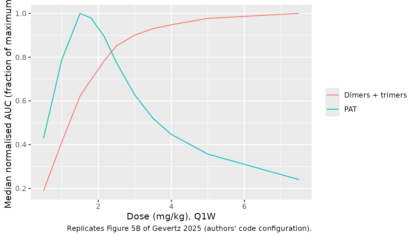
Figure 5B: dimers plus trimers
If every drug-bound complex in the bone marrow were active, the dose-response would be monotone (Emax-like) rather than bell-shaped.
fig5b <- sweep_code |>
  mutate(
    all_complexes = pmax(drug_cd3_bonemarrow + complex_bonemarrow + drug_bcma_bonemarrow +
      complex_cd3_sbcma_bonemarrow + trimer, 0),
    pat = pmax(trimer, 0)
  ) |>
  group_by(id, dose, freq_wk) |>
  summarise(
    auc_all = sum(diff(t) * (head(all_complexes, -1) + tail(all_complexes, -1)) / 2) / max(t),
    auc_pat = sum(diff(t) * (head(pat, -1) + tail(pat, -1)) / 2) / max(t),
    .groups = "drop"
  ) |>
  group_by(dose, freq_wk) |>
  summarise(across(c(auc_all, auc_pat), median), .groups = "drop")

ggplot(filter(fig5b, freq_wk == 1), aes(dose)) +
  geom_line(aes(y = auc_pat / max(auc_pat), colour = "PAT")) +
  geom_line(aes(y = auc_all / max(auc_all), colour = "Dimers + trimers")) +
  labs(
    x = "Dose (mg/kg), Q1W", y = "Median normalised AUC (fraction of maximum)", colour = NULL,
    caption = "Replicates Figure 5B of Gevertz 2025 (authors' code configuration)."
  )
Two-group stratification by baseline soluble BCMA
The paper splits virtual patients at the median plasma soluble BCMA at the end of the pre-equilibration (the first dose). Table S2 gives optimal doses of 1.5 (low sBCMA) and 2.5 (high sBCMA) mg/kg Q1W, and 3 and 3.5 mg/kg Q2W.
baseline <- sweep_code |>
  filter(t == 0, dose == doses[1], freq_wk == 1) |>
  distinct(vp, target, target_bcma_bonemarrow)
cut_sbcma <- median(baseline$target)
baseline <- baseline |> mutate(stratum = ifelse(target > cut_sbcma, "High sBCMA", "Low sBCMA"))

c(median_sBp = cut_sbcma, median_mBbm = median(baseline$target_bcma_bonemarrow))
#>  median_sBp median_mBbm
#>    18.33506    43.07561

strata <- as.data.frame(nca_code$result) |>
  filter(PPTESTCD == "auclast") |>
  left_join(arms |> select(id, vp), by = "id") |>
  left_join(baseline |> select(vp, stratum), by = "vp") |>
  group_by(stratum, freq_wk, dose) |>
  summarise(nauc = median(PPORRES) / horizon(freq_wk[1]), .groups = "drop")

strata |>
  group_by(stratum, freq_wk) |>
  summarise(optimal_dose = dose[which.max(nauc)], peak_nauc = max(nauc), .groups = "drop") |>
  mutate(table_s2 = c(1.5, 3, 2.5, 3.5)[match(paste(stratum, freq_wk), c(
    "Low sBCMA 1", "Low sBCMA 2", "High sBCMA 1", "High sBCMA 2"
  ))]) |>
  rename(
    Stratum = stratum, "Schedule (weeks)" = freq_wk, "Optimal dose (mg/kg)" = optimal_dose,
    "Peak normalised AUC (nM)" = peak_nauc, "Table S2 optimal dose (mg/kg)" = table_s2
  ) |>
knitr::kable(digits = 4)| Stratum | Schedule (weeks) | Optimal dose (mg/kg) | Peak normalised AUC (nM) | Table S2 optimal dose (mg/kg) |
|---|---|---|---|---|
| High sBCMA | 1 | 2.16 | 0.0557 | 2.5 |
| High sBCMA | 2 | 4.00 | 0.0590 | 3.5 |
| Low sBCMA | 1 | 1.50 | 0.0567 | 1.5 |
| Low sBCMA | 2 | 3.00 | 0.0572 | 3.0 |
ggplot(strata, aes(dose, nauc, colour = stratum)) +
  geom_line() +
  geom_point() +
  facet_wrap(~ paste0("Q", freq_wk, "W")) +
  labs(
    x = "Dose (mg/kg)", y = "Median normalised AUC of the PAT (nM)", colour = NULL,
    caption = "Replicates Figure S5 of Gevertz 2025 (authors' code configuration)."
  )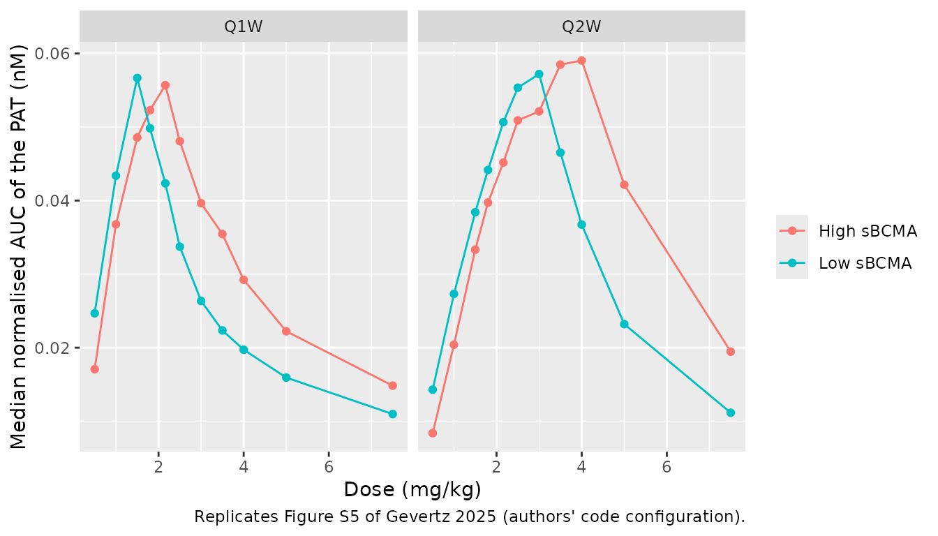
Figure S4 reports pre-treatment medians of 17.3 nM soluble BCMA in plasma and 42.3 nM membrane BCMA in the marrow, close to the medians above. As in Table S2, the low-sBCMA stratum is optimal at 1.5 mg/kg Q1W and 3 mg/kg Q2W, and the high-sBCMA optima fall inside the Table S2 ranges (1.5-2.5 mg/kg Q1W, 3-5 mg/kg Q2W). As in Figure S5, the high-sBCMA stratum reaches a higher PAT AUC and peaks at a dose at or above the low-sBCMA stratum.
PKNCA: free plasma drug at steady state
Girgis 2022, as quoted in the paper, predicts a steady-state trough of at least 6000 ng/mL at 0.72 mg/kg SC Q1W. The steady-state dosing interval (days 77-84 after the first step-up dose, the last of the ten treatment doses) is analysed below for the typical patient of each configuration.
ev_pk <- bind_rows(
  make_regimen(1, 0.72, 1, dt_obs = 0.1),
  make_regimen(2, 1.5, 1, dt_obs = 0.1)
)
pk <- bind_rows(
  solve_quiet(mod_code_typ, ev_pk) |> mutate(config = "Authors' code"),
  solve_quiet(mod_typ, ev_pk) |> mutate(config = "Table S1 (packaged)")
) |>
  mutate(t = time - t_eq, treatment = lab_fig2[as.character(id)], Cc = pmax(Cc, 0) * mw_kda) |>
  filter(!is.na(Cc)) |>
  select(config, treatment, id, t, Cc)
#> ℹ omega/sigma items treated as zero: 'etalcl_exp_inf', 'etalkshed', 'etalbl_mbcma_bm', 'etalktr_ab_c_bm', 'etalbl_cd3_bm'
#> ℹ omega/sigma items treated as zero: 'etalcl_exp_inf', 'etalkshed', 'etalbl_mbcma_bm', 'etalktr_ab_c_bm', 'etalbl_cd3_bm'
pk <- bind_rows(pk, pk |> distinct(config, treatment, id) |> mutate(t = 0, Cc = 0)) |>
  distinct(config, treatment, id, t, .keep_all = TRUE) |>
  arrange(config, treatment, id, t)

dose_pk <- ev_pk |>
  filter(evid == 1) |>
  mutate(t = time - t_eq, treatment = lab_fig2[as.character(id)]) |>
  tidyr::crossing(config = c("Authors' code", "Table S1 (packaged)")) |>
  select(config, treatment, id, t, amt)

conc_obj <- PKNCA::PKNCAconc(pk, Cc ~ t | config + treatment + id)
dose_obj <- PKNCA::PKNCAdose(dose_pk, amt ~ t | config + treatment + id)
intervals <- data.frame(start = 77, end = 84, cmax = TRUE, cmin = TRUE, cav = TRUE)
nca_pk <- PKNCA::pk.nca(PKNCA::PKNCAdata(conc_obj, dose_obj, intervals = intervals))

cmp_pk <- nlmixr2lib::ncaComparisonTable(
  simulated = as.data.frame(nca_pk$result) |> filter(config == "Authors' code", treatment == "0.72 mg/kg SC Q1W"),
  reference = data.frame(cmin = 6000),
  params = "cmin",
  units = c(cmin = "ng/mL"),
  tolerance_pct = 20
)
knitr::kable(cmp_pk, caption = "Steady-state trough at 0.72 mg/kg Q1W, authors' code configuration vs the Girgis 2022 benchmark quoted in the paper. * differs by >20%.")| NCA parameter | Reference | Simulated | % diff |
|---|---|---|---|
| Cmin (ng/mL) | 6000 | 6260 | +4.3% |
as.data.frame(nca_pk$result) |>
  filter(PPTESTCD %in% c("cmax", "cmin", "cav")) |>
  select(config, treatment, PPTESTCD, PPORRES) |>
  pivot_wider(names_from = PPTESTCD, values_from = PPORRES) |>
  rename(
    Configuration = config, Regimen = treatment,
    "Cmax (ng/mL)" = cmax, "Cmin (ng/mL)" = cmin, "Cav (ng/mL)" = cav
  ) |>
knitr::kable(digits = 0)| Configuration | Regimen | Cmax (ng/mL) | Cmin (ng/mL) | Cav (ng/mL) |
|---|---|---|---|---|
| Authors’ code | 0.72 mg/kg SC Q1W | 8913 | 6259 | 7949 |
| Authors’ code | 1.5 mg/kg SC Q1W | 19581 | 14048 | 17571 |
| Table S1 (packaged) | 0.72 mg/kg SC Q1W | 8236 | 5603 | 7273 |
| Table S1 (packaged) | 1.5 mg/kg SC Q1W | 18086 | 12587 | 16075 |
The Girgis benchmark comes from a different model and a different simulated patient, so it is a plausibility check rather than an identity.
Assumptions and deviations
-
Published table and equations versus the authors’
code. The packaged model follows Table S1 and the printed Eqs
(1)-(18). The authors’ MATLAB code, which produced every published
figure, differs as follows. The maintainers ship the printed values and
rebuild the code configuration in this article (
mod_codeabove):-
kint_bcma(kint,mB): Table S1 2/day; code0.693 / 1.25= 0.554/day (a 30 h BCMA half-life, inside the 24-36 h the Methods quote). This is the difference that moves the PAT peak. -
kint_cd3(kint3): Table S1 16.6/day; code 1.584/day. -
lcl_exp_inf(Cl1): Table S1 0.5 L/day; code 0.449 L/day (Miao 2023 CL1, and the Figure S2A mean of 6.0676 mL/kg/day at 74 kg). - Association rates: Table S1 10 and 111 1/nM/day; code
koff / KD= 10.17 and 111.1 1/nM/day. - Eqs (7) and (9): the plasma drug-sBCMA dimer and inactive trimer are
cleared at
k10,sB; the code clears them at the drug elimination ratek10. - Eq (11): soluble BCMA enters the marrow at
kB,1bm sBp; the code uses(V1 / Vbm) k1bm sBp, which conserves mass across the two volumes and uses the drug’s (virtual-patient-specific) distribution rate. - Eq (15): the bone-marrow drug-sBCMA dimer has no clearance; the code
clears it at
kout.
-
-
Synthesis rates. Table S1 lists
ksyn,mB = 19.8andksyn,bm = 19.8nM/day, which disagree with the Data S1 definitionsksyn,mB = mBbm(0) (kint,mB + kshed)andksyn,CD3 = CD3bm(0) kint3(102.5 and 1.66 nM/day with the Table S1 rates). The model uses the definitions, which hold each target at its baseline as the text intends. The tabulated 19.8 equals50 (log(2) / 2 + 0.05), which suggests an earlier BCMA half-life of 2 days; the code computes all three synthesis rates from the definitions. -
V1. Table S1 gives “3-4 L”. The tabulated
k10 = Cl1 / V1 = 0.17andk12 = Cl2 / V1 = 0.13both require 3 L, as does the code. -
Time-dependent clearance. Table S1 writes
Cl1 = Clvar exp(-delta t)with Clvar from Miao 2023. The model implementsCl1 + Clvar exp(-delta t)with Clvar = 0.547 L/day, which is how the code applies it and matches the additive decomposition of Miao 2023.tis time since the first dose. -
Peripheral elimination. Eq (6) eliminates drug from
the peripheral compartment at
k10as well as from plasma. This is carried as printed (the code does the same). -
Bone-marrow CD3 binding. Eqs (12)-(18) use
kon3,bmandkoff3,bm, which Table S1 does not list. The plasma values are used, as in the code. - Initial conditions and pre-equilibration. The model starts from the Table S1 initial conditions, which are not a steady state; the authors solve the drug-free system for 50 days before the first dose, and doses should be given at day 50 to reproduce the paper. The soluble BCMA pools are still drifting at day 50 (the slowest mode has a half-life of about 40 days), so the baseline depends on the equilibration length, as it does in the paper.
-
Virtual-patient code details. In the dose-sweep
code the authors equilibrate each virtual patient with
ksyn,mB = kint,mB mBbm(0)(no shedding term) and then reset membrane BCMA and bone-marrow CD3 to the virtual patient’s values at the first dose. These steps are not reproduced here; they lower the pre-treatment soluble BCMA slightly (Figure S4 median 17.3 nM against 18.3 nM here). - Body weight. The paper does not state a body weight; mg/kg doses are converted at the 74 kg used in the authors’ code (also the Miao 2023 reference weight).
-
Virtual population. The model’s etas are
median-centred; the paper’s draws are mean-preserving, so this article
samples etas from
N(-omega^2 / 2, omega^2). 100 virtual patients per arm are used instead of 1200, and 11 of the 20 swept doses. -
Residual error. The paper’s simulations are
deterministic;
propSdis fixed to 0. - No erratum or correction notice for the article was found (checked 2026-11-11).