Apremilast popPK and PASI / sPGA exposure-response in Japanese and non-Japanese psoriasis (Okubo 2021)
Source:vignettes/articles/Okubo_2021_apremilast.Rmd
Okubo_2021_apremilast.RmdModel and source
Okubo 2021 reports a population PK (PPK) model of oral apremilast, a phosphodiesterase 4 inhibitor, fitted to pooled Japanese and non-Japanese data, followed by three exposure-response (E-R) models that link the individual steady-state AUC from that PPK model to clinical response. Each is packaged as its own model:
-
Okubo_2021_apremilast: the one-compartment PPK model (Table 4). -
Okubo_2021_apremilast_pasi75: longitudinal logistic E-R model for PASI-75 (Table S2). -
Okubo_2021_apremilast_pasi50: longitudinal logistic E-R model for PASI-50 (Table S2). -
Okubo_2021_apremilast_spga: longitudinal logistic E-R model for sPGA response (score 0 or 1) (Table S2).
nms <- c(
  "Okubo_2021_apremilast", "Okubo_2021_apremilast_pasi75",
  "Okubo_2021_apremilast_pasi50", "Okubo_2021_apremilast_spga"
)
uis <- setNames(lapply(nms, function(n) rxode2::rxode(readModelDb(n))), nms)
#> ℹ parameter labels from comments will be replaced by 'label()'- Citation: Okubo Y, Ohtsuki M, Komine M, Imafuku S, Kassir N, Petric R, Nemoto O. Population pharmacokinetic and exposure-response analysis of apremilast in Japanese subjects with moderate to severe psoriasis. J Dermatol. 2021;48(11):1652-1664. doi:10.1111/1346-8138.16068
- Article: https://doi.org/10.1111/1346-8138.16068 (open access; the supporting information holds Tables S1-S3, Appendices S1-S5 and Figures S1-S3)
Population
The PPK analysis pooled 5704 quantifiable apremilast concentrations from 517 subjects in nine studies (Okubo 2021 Results 3.2 and Table 1): 104 Japanese adults with moderate to severe plaque psoriasis in the phase 2b study PSOR-011 (apremilast 20 or 30 mg twice daily), 233 non-Japanese psoriasis patients in the phase 2b PSOR-005 (10, 20 or 30 mg twice daily) and phase 3 PSOR-008/ESTEEM 1 (30 mg twice daily) studies, and 180 non-Japanese subjects in six phase 1 studies (mostly healthy adults; one study in patients with psoriasis, psoriatic arthritis or rheumatoid arthritis on methotrexate). Study-level baseline demographics are in Okubo 2021 Table 3: Japanese patients averaged 51.4 years and 70.2 kg (75% male), while the non-Japanese psoriasis patients averaged 46.5-49.1 years and about 95 kg (63-69% male). Overall 359 of 517 subjects (69%) were male.
The E-R models used 9087 PASI-75 / PASI-50 observations from 1433 subjects and 9094 sPGA observations from 1442 subjects in PSOR-005, PSOR-008/ESTEEM 1 and PSOR-011, over weeks 2-24, 2-16 and 2-40 respectively (Methods 2.5, Results 3.3).
str(uis[["Okubo_2021_apremilast"]]$population)
#> List of 11
#>  $ species       : chr "human"
#>  $ n_subjects    : int 517
#>  $ n_studies     : int 9
#>  $ age_range     : chr "Study means 28.0-52.4 years; PK-024 enrolled healthy adults 65-85 years (Okubo 2021 Tables 1 and 3)"
#>  $ weight_range  : chr "Study means 70.2-96.3 kg (Okubo 2021 Table 3)"
#>  $ sex_female_pct: num 30.6
#>  $ race_ethnicity: Named num [1:4] 20.1 66.7 10.4 2.7
#>   ..- attr(*, "names")= chr [1:4] "Japanese" "Caucasian" "Black" "Other"
#>  $ disease_state : chr "Moderate to severe plaque psoriasis (104 Japanese patients in PSOR-011; 233 non-Japanese patients in PSOR-005 a"| __truncated__
#>  $ dose_range    : chr "Oral apremilast 10, 20 or 30 mg twice daily (phase 2b/3); 20-50 mg single or 30-50 mg twice-daily doses (phase 1)."
#>  $ regions       : chr "Japan, USA, Canada, UK, Europe, Australia"
#>  $ notes         : chr "Okubo 2021 Results 3.2: 5752 samples from 517 subjects, 48 below the LOQ of 1.00 ng/mL excluded, leaving 5704 ("| __truncated__
Source trace
Every ini() value carries an in-file comment naming its
source; the table collects them.
| Model | Parameter / equation | Value | Source location |
|---|---|---|---|
| PPK |
lcl (CL/F, healthy female non-Japanese, 45 y) |
log(9.25) L/h | Table 4 |
| PPK |
lvc (Vc/F at 82 kg) |
log(115) L | Table 4 |
| PPK |
lka (Ka) |
log(1.83) 1/h | Table 4 |
| PPK |
ltlag (lag time) |
log(0.290) h | Table 4 |
| PPK | e_dis_psoriasis_cl |
0.834 | Table 4, footnote a |
| PPK |
e_sexm_cl (male) |
1.25 | Table 4, footnote b |
| PPK | e_race_japanese_cl |
1.17 | Table 4, footnote c |
| PPK |
e_age_cl on (AGE/45) |
-0.148 | Table 4, footnote d |
| PPK |
e_wt_vc on (WT/82) |
0.591 | Table 4, footnote e |
| PPK |
etalcl, etalvc, etalka
|
38.0%, 27.1%, 83.4% CV | Table 4 (converted with log(1 + CV^2)) |
| PPK |
propSd, addSd
|
0.365, 0.658 ng/mL | Table 4 ‘Error model’ |
| PPK | One compartment, first-order absorption with lag | n/a | Results 3.2; Appendix S2-S3 |
| PASI-75 |
bsl_pbo, asym_pbo, lkpbo
|
-7.83, 5.38, log(0.183) 1/week | Table S2 |
| PASI-75 |
emax, lauc50
|
3.38, log(1733) ng*h/mL
|
Table S2 |
| PASI-50 |
bsl_pbo, asym_pbo, lkpbo
|
-5.84, 4.50, log(0.282) 1/week | Table S2 |
| PASI-50 |
emax, lauc50
|
2.91, log(1656) ng*h/mL
|
Table S2 |
| sPGA |
bsl_pbo, asym_pbo, lkpbo
|
-8.81, 5.87, log(0.579) 1/week | Table S2 |
| sPGA |
emax, lauc50
|
4.58, log(1110) ng*h/mL
|
Table S2 |
| sPGA |
e_race_japanese_bsl_pbo, _asym_pbo,
_emax
|
0.682, 0.716, 0.661 | Table S2 ‘If Japanese’ rows |
| sPGA |
lkdrug (drug-effect onset) |
log(0.0540) 1/week | Not printed; back-solved from Table S1 and Results 3.3 (see below) |
| E-R | logit = intercept + placebo x (1 - exp(-K t)) + Emax x AUC / (E50 + AUC) | n/a | Appendix S5; Table S2 definitions |
Population PK
Covariate effects quoted in the text
Results 3.2 translates each covariate effect into a percentage change. These follow from the encoded coefficients alone, so they are checked to the rounding of the printed percentages.
th <- uis[["Okubo_2021_apremilast"]]$theta
claims <- tibble::tribble(
  ~claim, ~model, ~paper,
  "Vc/F at 45.5 kg vs 82 kg", (45.5 / 82)^th[["e_wt_vc"]], 1 - 0.29,
  "Vc/F at 102 kg vs 82 kg", (102 / 82)^th[["e_wt_vc"]], 1 + 0.14,
  "CL/F at 19 y vs 45 y", (19 / 45)^th[["e_age_cl"]], 1 + 0.14,
  "CL/F at 80 y vs 45 y", (80 / 45)^th[["e_age_cl"]], 1 - 0.08,
  "CL/F psoriasis vs healthy", th[["e_dis_psoriasis_cl"]], 1 - 0.17,
  "CL/F male vs female", th[["e_sexm_cl"]], 1.25,
  "CL/F Japanese vs non-Japanese", th[["e_race_japanese_cl"]], 1.17
)
knitr::kable(claims, digits = 3, caption = "Covariate ratios: model vs Okubo 2021 Results 3.2.")| claim | model | paper |
|---|---|---|
| Vc/F at 45.5 kg vs 82 kg | 0.706 | 0.71 |
| Vc/F at 102 kg vs 82 kg | 1.138 | 1.14 |
| CL/F at 19 y vs 45 y | 1.136 | 1.14 |
| CL/F at 80 y vs 45 y | 0.918 | 0.92 |
| CL/F psoriasis vs healthy | 0.834 | 0.83 |
| CL/F male vs female | 1.250 | 1.25 |
| CL/F Japanese vs non-Japanese | 1.170 | 1.17 |
Typical-value steady state
For a linear one-compartment model the steady-state AUC over one dosing interval is exactly dose / CL. A typical Japanese male psoriasis patient (51 years, 70 kg) at 30 mg twice daily is solved to steady state and the simulated AUCtau is compared with that closed form.
mod_pk <- readModelDb("Okubo_2021_apremilast")
tau <- 12
n_dose <- 28
t_last <- (n_dose - 1) * tau
obs_grid <- t_last + c(0, 0.25, 0.5, 0.75, 1, 1.5, 2, 2.5, 3, 4, 5, 6, 8, 10, 12)

typ <- data.frame(WT = 70, AGE = 51, SEXF = 0, RACE_JAPANESE = 1, DIS_PSORIASIS = 1)
ev_typ <- bind_rows(
  data.frame(id = 1L, time = (seq_len(n_dose) - 1) * tau, amt = 30, evid = 1L, cmt = "depot"),
  data.frame(id = 1L, time = obs_grid, amt = 0, evid = 0L, cmt = "central")
) |>
  arrange(time, desc(evid)) |>
  cross_join(typ)
sim_typ <- rxode2::rxSolve(rxode2::zeroRe(mod_pk), events = ev_typ,
                           rtol = 1e-10, atol = 1e-12, returnType = "data.frame")
#> ℹ parameter labels from comments will be replaced by 'label()'
#> ℹ omega/sigma items treated as zero: 'etalcl', 'etalvc', 'etalka'
cl_typ <- sim_typ$cl[1]
auc_typ <- with(sim_typ, sum(diff(time) * (head(Cc, -1) + tail(Cc, -1)) / 2))
auc_exact <- 1000 * 30 / cl_typ
c(CL_L_per_h = cl_typ, AUCtau_trapezoid = auc_typ, AUCtau_dose_over_CL = auc_exact)
#>          CL_L_per_h    AUCtau_trapezoid AUCtau_dose_over_CL
#>            11.07538          2710.10685          2708.71012
# 28 doses at a 7.5 h half-life is steady state to < 1e-10; the residual is
# the linear-trapezoid error on the 15-point grid, measured at about 0.05%.
stopifnot(abs(auc_typ / auc_exact - 1) < 0.005)
Virtual cohort
Observed data are not public. Virtual psoriasis cohorts follow the Table 3 study means and CVs for PSOR-011 (Japanese) and PSOR-005 / PSOR-008 (non-Japanese); age and weight are drawn from normal distributions truncated to plausible adult ranges. 150 subjects per arm.
set.seed(20211116)
n_arm <- 150
arms <- tibble::tribble(
  ~treatment, ~dose_mg, ~japanese, ~age_m, ~age_cv, ~wt_m, ~wt_cv, ~male,
  "Japanese 20 mg BID", 20, 1L, 51.4, 0.241, 70.2, 0.182, 0.750,
  "Japanese 30 mg BID", 30, 1L, 51.4, 0.241, 70.2, 0.182, 0.750,
  "PSOR-005 10 mg BID", 10, 0L, 46.5, 0.286, 96.3, 0.223, 0.627,
  "PSOR-005 20 mg BID", 20, 0L, 46.5, 0.286, 96.3, 0.223, 0.627,
  "PSOR-005 30 mg BID", 30, 0L, 46.5, 0.286, 96.3, 0.223, 0.627,
  "ESTEEM 1 30 mg BID", 30, 0L, 49.1, 0.276, 94.9, 0.212, 0.687
)
rtrunc <- function(n, m, s, lo, hi) {
  x <- rnorm(n, m, s)
  while (any(bad <- x < lo | x > hi)) x[bad] <- rnorm(sum(bad), m, s)
  x
}
cohort <- arms |>
  mutate(arm = row_number()) |>
  rowwise() |>
  reframe(
    treatment = treatment, dose_mg = dose_mg, RACE_JAPANESE = japanese,
    AGE = rtrunc(n_arm, age_m, age_m * age_cv, 20, 85),
    WT = rtrunc(n_arm, wt_m, wt_m * wt_cv, 40, 180),
    SEXF = as.integer(runif(n_arm) > male)
  ) |>
  mutate(id = row_number(), DIS_PSORIASIS = 1L)

events <- bind_rows(
  cohort |> cross_join(data.frame(time = (seq_len(n_dose) - 1) * tau)) |>
    mutate(amt = dose_mg, evid = 1L, cmt = "depot"),
  cohort |> cross_join(data.frame(time = obs_grid)) |>
    mutate(amt = 0, evid = 0L, cmt = "central")
) |>
  arrange(id, time, desc(evid))
stopifnot(n_distinct(events$id) == nrow(arms) * n_arm)Figure 3: CL/F in Japanese vs non-Japanese psoriasis patients
indiv <- sim |>
  distinct(id, treatment, dose_mg, cl, vc) |>
  mutate(population = ifelse(grepl("^Japanese", treatment), "Japanese", "Non-Japanese"))
ggplot(indiv, aes(population, cl)) +
  geom_boxplot(outlier.shape = NA) +
  geom_jitter(width = 0.15, alpha = 0.2, size = 0.6) +
  labs(x = NULL, y = "CL/F (L/h)",
       caption = "Replicates Figure 3 of Okubo 2021 (virtual cohort).")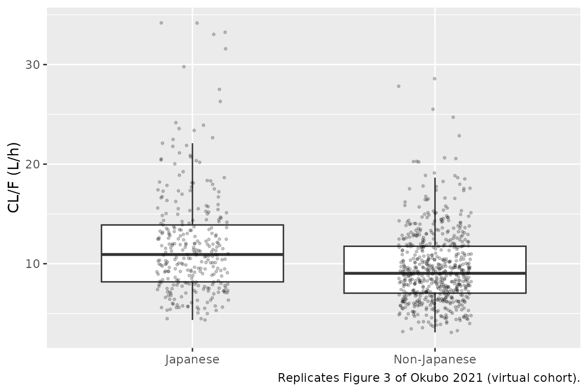
indiv |>
  group_by(population) |>
  summarise(median_CL = median(cl), .groups = "drop") |>
knitr::kable(digits = 2, caption = "Median simulated CL/F by population.")| population | median_CL |
|---|---|
| Japanese | 10.93 |
| Non-Japanese | 9.04 |
Figure 4: steady-state profiles
sim |>
  filter(dose_mg %in% c(20, 30), !grepl("ESTEEM", treatment)) |>
  mutate(
    population = ifelse(grepl("^Japanese", treatment), "Japanese", "Non-Japanese (PSOR-005)"),
    regimen = paste(dose_mg, "mg BID"),
    tad = time - t_last
  ) |>
  group_by(population, regimen, tad) |>
  summarise(
    Q05 = quantile(Cc, 0.05), Q50 = median(Cc), Q95 = quantile(Cc, 0.95),
    .groups = "drop"
  ) |>
  ggplot(aes(tad, Q50, colour = population, fill = population)) +
  geom_ribbon(aes(ymin = Q05, ymax = Q95), alpha = 0.15, colour = NA) +
  geom_line() +
  facet_wrap(~regimen) +
  labs(x = "Time after morning dose at steady state (h)",
       y = "Apremilast (ng/mL)", colour = NULL, fill = NULL,
       caption = "Replicates Figure 4 of Okubo 2021: median and 90% interval.")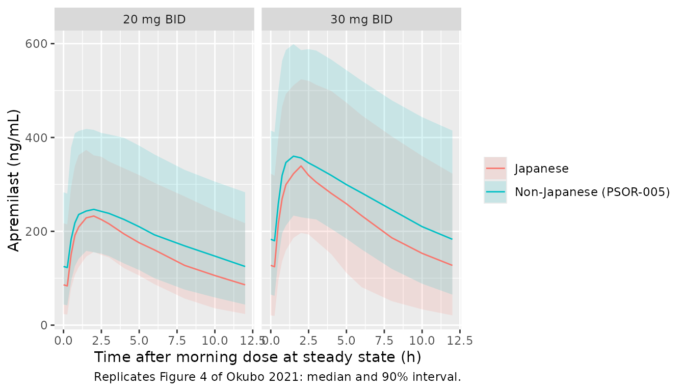
PKNCA: steady-state exposure
sim_nca <- sim |>
  filter(!is.na(Cc)) |>
  select(id, time, Cc, treatment)
dose_df <- events |>
  filter(evid == 1) |>
  select(id, time, amt, treatment)
conc_obj <- PKNCA::PKNCAconc(sim_nca, Cc ~ time | treatment + id)
dose_obj <- PKNCA::PKNCAdose(dose_df, amt ~ time | treatment + id)
intervals <- data.frame(
  start = t_last, end = t_last + tau,
  cmax = TRUE, cmin = TRUE, tmax = TRUE, auclast = TRUE
)
nca_res <- PKNCA::pk.nca(PKNCA::PKNCAdata(conc_obj, dose_obj, intervals = intervals))
Okubo 2021 Table 5 gives the model-predicted geometric means of AUCtau,ss, Cmax,ss and Cmin,ss in the E-R populations; these are the most direct check of the encoded model.
table5 <- tibble::tribble(
  ~treatment, ~auclast, ~cmax, ~cmin,
  "Japanese 20 mg BID", 1939.2, 240.3, 87.2,
  "Japanese 30 mg BID", 2727.2, 341.8, 120.3,
  "PSOR-005 10 mg BID", 1098.9, 124.0, 58.7,
  "PSOR-005 20 mg BID", 2185.2, 247.7, 115.6,
  "PSOR-005 30 mg BID", 3337.2, 376.7, 178.3,
  "ESTEEM 1 30 mg BID", 3352.4, 377.0, 179.9
)
cmp5 <- nlmixr2lib::ncaComparisonTable(
  simulated = nca_res,
  reference = table5,
  by = "treatment",
  params = c("auclast", "cmax", "cmin"),
  units = c(auclast = "ng*h/mL", cmax = "ng/mL", cmin = "ng/mL"),
  tolerance_pct = 20
)
knitr::kable(cmp5, caption = "Simulated (median) vs Okubo 2021 Table 5 (model-predicted geometric mean). * differs by >20%.")| NCA parameter | treatment | Reference | Simulated | % diff |
|---|---|---|---|---|
| Cmax (ng/mL) | Japanese 20 mg BID | 240 | 240 | -0.1% |
| Cmax (ng/mL) | Japanese 30 mg BID | 342 | 348 | +1.8% |
| Cmax (ng/mL) | PSOR-005 10 mg BID | 124 | 123 | -0.8% |
| Cmax (ng/mL) | PSOR-005 20 mg BID | 248 | 251 | +1.2% |
| Cmax (ng/mL) | PSOR-005 30 mg BID | 377 | 367 | -2.6% |
| Cmax (ng/mL) | ESTEEM 1 30 mg BID | 377 | 379 | +0.6% |
| Cmin (ng/mL) | Japanese 20 mg BID | 87.2 | 83.7 | -4.0% |
| Cmin (ng/mL) | Japanese 30 mg BID | 120 | 125 | +3.5% |
| Cmin (ng/mL) | PSOR-005 10 mg BID | 58.7 | 56.6 | -3.6% |
| Cmin (ng/mL) | PSOR-005 20 mg BID | 116 | 123 | +6.2% |
| Cmin (ng/mL) | PSOR-005 30 mg BID | 178 | 180 | +0.9% |
| Cmin (ng/mL) | ESTEEM 1 30 mg BID | 180 | 191 | +6.3% |
| AUClast (ng*h/mL) | Japanese 20 mg BID | 1940 | 1840 | -5.3% |
| AUClast (ng*h/mL) | Japanese 30 mg BID | 2730 | 2670 | -2.1% |
| AUClast (ng*h/mL) | PSOR-005 10 mg BID | 1100 | 1070 | -2.6% |
| AUClast (ng*h/mL) | PSOR-005 20 mg BID | 2190 | 2320 | +6.3% |
| AUClast (ng*h/mL) | PSOR-005 30 mg BID | 3340 | 3240 | -2.9% |
| AUClast (ng*h/mL) | ESTEEM 1 30 mg BID | 3350 | 3400 | +1.4% |
nca_df <- as.data.frame(nca_res)
auc_med <- nca_df |>
  filter(PPTESTCD == "auclast") |>
  group_by(treatment) |>
  summarise(sim = median(PPORRES), .groups = "drop") |>
  left_join(table5 |> select(treatment, ref = auclast), by = "treatment") |>
  mutate(pct_diff = 100 * (sim / ref - 1))
auc_med
#> # A tibble: 6 × 4
#>   treatment            sim   ref pct_diff
#>   <chr>              <dbl> <dbl>    <dbl>
#> 1 ESTEEM 1 30 mg BID 3398. 3352.     1.38
#> 2 Japanese 20 mg BID 1836. 1939.    -5.31
#> 3 Japanese 30 mg BID 2670. 2727.    -2.11
#> 4 PSOR-005 10 mg BID 1070. 1099.    -2.62
#> 5 PSOR-005 20 mg BID 2323. 2185.     6.29
#> 6 PSOR-005 30 mg BID 3239. 3337.    -2.95
# Structural: a wrong CL, covariate factor or unit moves AUC by tens of
# percent. The cohort is a demographic approximation, so the arm medians
# are compared to the centre of Table 5, not to its extremes.
stopifnot(abs(median(auc_med$pct_diff)) < 10, max(abs(auc_med$pct_diff)) < 20)
Okubo 2021 Table 2 also reports the observed non-compartmental week-20 values in the intensive-sampling Japanese subset (n = 21 and 20). They are shown for context only: the subset is small, AUCtau rises less than dose-proportionally between 20 and 30 mg in those data, and the trapezoid AUCtau there extrapolates the 12 h concentration from 8 h. The model’s own predictions in Table 5 sit below the observed 20 mg Cmax as well (240 vs 304 ng/mL), so the starred 20 mg Cmax row reflects that subset rather than the encoding.
table2 <- tibble::tribble(
  ~treatment, ~auclast, ~cmax, ~cmin, ~tmax,
  "Japanese 20 mg BID", 1957, 304, 90.8, 2.03,
  "Japanese 30 mg BID", 2397, 374, 104, 2.00
)
cmp2 <- nlmixr2lib::ncaComparisonTable(
  simulated = nca_res,
  reference = table2,
  by = "treatment",
  params = c("auclast", "cmax", "cmin", "tmax"),
  units = c(auclast = "ng*h/mL", cmax = "ng/mL", cmin = "ng/mL", tmax = "h"),
  tolerance_pct = 20
)
cmp2 <- cmp2[grepl("^Japanese", cmp2$treatment), ]
knitr::kable(cmp2, caption = "Simulated (median) vs Okubo 2021 Table 2 (observed NCA, Japanese, week 20). * differs by >20%.")| NCA parameter | treatment | Reference | Simulated | % diff |
|---|---|---|---|---|
| Cmax (ng/mL) | Japanese 20 mg BID | 304 | 240 | -21.1%* |
| Cmax (ng/mL) | Japanese 30 mg BID | 374 | 348 | -6.9% |
| Cmin (ng/mL) | Japanese 20 mg BID | 90.8 | 83.7 | -7.8% |
| Cmin (ng/mL) | Japanese 30 mg BID | 104 | 125 | +19.7% |
| Tmax (h) | Japanese 20 mg BID | 2.03 | 2 | -1.5% |
| Tmax (h) | Japanese 30 mg BID | 2 | 2 | +0.0% |
| AUClast (ng*h/mL) | Japanese 20 mg BID | 1960 | 1840 | -6.2% |
| AUClast (ng*h/mL) | Japanese 30 mg BID | 2400 | 2670 | +11.4% |
Exposure-response
Week-16 probabilities (Table S1 and Results 3.3)
The E-R models are logistic in the logit
intercept + placebo x (1 - exp(-K t)) + Emax x AUC / (E50 + AUC)
with t in weeks and AUC the individual
AUCtau,ss. Okubo 2021 prints 29 week-16 response probabilities at fixed
AUC values (Table S1 and Results 3.3). The models are deterministic
given the AUC, so each printed value is reproduced to its one-decimal
rounding.
printed <- tibble::tribble(
  ~endpoint, ~RACE_JAPANESE, ~AUC_APREMILAST, ~paper_pct, ~source,
  "pasi75", 0L, 0, 6.1, "Table S1 placebo",
  "pasi75", 0L, 1065.4, 19.0, "Results 3.3 / Table S1",
  "pasi75", 0L, 2030.6, 28.6, "Results 3.3",
  "pasi75", 0L, 3169.2, 36.5, "Results 3.3",
  "pasi75", 0L, 2136.5, 29.5, "Table S1",
  "pasi75", 0L, 3213.4, 36.8, "Table S1",
  "pasi75", 1L, 1840.5, 27.0, "Table S1",
  "pasi75", 1L, 2720.3, 33.8, "Table S1",
  "pasi75", 1L, 1065.4, 19.0, "Table S1",
  "pasi50", 0L, 0, 20.0, "Table S1 placebo",
  "pasi50", 0L, 1065.4, 43.8, "Results 3.3 / Table S1",
  "pasi50", 0L, 2030.6, 55.3, "Results 3.3",
  "pasi50", 0L, 3169.2, 62.8, "Results 3.3",
  "pasi50", 0L, 2136.5, 56.2, "Table S1",
  "pasi50", 0L, 3213.4, 63.0, "Table S1",
  "pasi50", 1L, 1840.5, 53.6, "Table S1",
  "pasi50", 1L, 2720.3, 60.3, "Table S1",
  "spga", 0L, 0, 5.0, "Table S1 placebo",
  "spga", 1L, 0, 14.1, "Table S1 placebo",
  "spga", 0L, 1065.4, 16.2, "Results 3.3 / Table S1",
  "spga", 0L, 2030.6, 22.7, "Results 3.3",
  "spga", 0L, 3169.2, 27.3, "Results 3.3",
  "spga", 0L, 2136.5, 23.2, "Table S1",
  "spga", 0L, 3213.4, 27.5, "Table S1",
  "spga", 1L, 1065.4, 27.9, "Table S1",
  "spga", 1L, 1840.5, 32.9, "Table S1",
  "spga", 1L, 2720.3, 36.3, "Table S1",
  "spga", 1L, 2030.6, 33.8, "Results 3.3",
  "spga", 1L, 3169.2, 37.5, "Results 3.3"
)

er_models <- list(
  pasi75 = readModelDb("Okubo_2021_apremilast_pasi75"),
  pasi50 = readModelDb("Okubo_2021_apremilast_pasi50"),
  spga = readModelDb("Okubo_2021_apremilast_spga")
)
er_out <- c(pasi75 = "prob_pasi75", pasi50 = "prob_pasi50", spga = "prob_spga01")

# Solve one E-R model on a data frame of observation rows (one row per id).
# The E-R models have no random effects by design (Table S2), so rxode2's
# notice about a multi-subject solve without omega is expected and muffled.
muffle_no_omega <- function(w) {
  if (grepl("without 'omega'", conditionMessage(w))) invokeRestart("muffleWarning")
}
solve_er <- function(endpoint, df) {
  ev <- df |> mutate(evid = 0L, amt = 0)
  out <- withCallingHandlers(
    rxode2::rxSolve(er_models[[endpoint]], events = ev, returnType = "data.frame"),
    warning = muffle_no_omega
  )
  if (is.null(out$id)) out$id <- 1L
  stopifnot(nrow(out) == nrow(ev))
  out[[er_out[[endpoint]]]][match(ev$id, out$id)]
}

printed <- printed |>
  group_by(endpoint) |>
  group_modify(function(d, k) {
    d$model_pct <- 100 * solve_er(
      k$endpoint,
      d |> mutate(id = row_number(), time = 16) |> select(id, time, AUC_APREMILAST, RACE_JAPANESE)
    )
    d
  }) |>
  ungroup() |>
  mutate(diff_pp = model_pct - paper_pct)
knitr::kable(printed, digits = 2, caption = "Week-16 response probability (%): model vs Okubo 2021.")| endpoint | RACE_JAPANESE | AUC_APREMILAST | paper_pct | source | model_pct | diff_pp |
|---|---|---|---|---|---|---|
| pasi50 | 0 | 0.0 | 20.0 | Table S1 placebo | 19.95 | -0.05 |
| pasi50 | 0 | 1065.4 | 43.8 | Results 3.3 / Table S1 | 43.78 | -0.02 |
| pasi50 | 0 | 2030.6 | 55.3 | Results 3.3 | 55.32 | 0.02 |
| pasi50 | 0 | 3169.2 | 62.8 | Results 3.3 | 62.76 | -0.04 |
| pasi50 | 0 | 2136.5 | 56.2 | Table S1 | 56.22 | 0.02 |
| pasi50 | 0 | 3213.4 | 63.0 | Table S1 | 62.97 | -0.03 |
| pasi50 | 1 | 1840.5 | 53.6 | Table S1 | 53.55 | -0.05 |
| pasi50 | 1 | 2720.3 | 60.3 | Table S1 | 60.34 | 0.04 |
| pasi75 | 0 | 0.0 | 6.1 | Table S1 placebo | 6.08 | -0.02 |
| pasi75 | 0 | 1065.4 | 19.0 | Results 3.3 / Table S1 | 18.98 | -0.02 |
| pasi75 | 0 | 2030.6 | 28.6 | Results 3.3 | 28.61 | 0.01 |
| pasi75 | 0 | 3169.2 | 36.5 | Results 3.3 | 36.52 | 0.02 |
| pasi75 | 0 | 2136.5 | 29.5 | Table S1 | 29.49 | -0.01 |
| pasi75 | 0 | 3213.4 | 36.8 | Table S1 | 36.77 | -0.03 |
| pasi75 | 1 | 1840.5 | 27.0 | Table S1 | 26.95 | -0.05 |
| pasi75 | 1 | 2720.3 | 33.8 | Table S1 | 33.78 | -0.02 |
| pasi75 | 1 | 1065.4 | 19.0 | Table S1 | 18.98 | -0.02 |
| spga | 0 | 0.0 | 5.0 | Table S1 placebo | 5.02 | 0.02 |
| spga | 1 | 0.0 | 14.1 | Table S1 placebo | 14.11 | 0.01 |
| spga | 0 | 1065.4 | 16.2 | Results 3.3 / Table S1 | 16.21 | 0.01 |
| spga | 0 | 2030.6 | 22.7 | Results 3.3 | 22.66 | -0.04 |
| spga | 0 | 3169.2 | 27.3 | Results 3.3 | 27.32 | 0.02 |
| spga | 0 | 2136.5 | 23.2 | Table S1 | 23.20 | 0.00 |
| spga | 0 | 3213.4 | 27.5 | Table S1 | 27.46 | -0.04 |
| spga | 1 | 1065.4 | 27.9 | Table S1 | 27.93 | 0.03 |
| spga | 1 | 1840.5 | 32.9 | Table S1 | 32.89 | -0.01 |
| spga | 1 | 2720.3 | 36.3 | Table S1 | 36.31 | 0.01 |
| spga | 1 | 2030.6 | 33.8 | Results 3.3 | 33.77 | -0.03 |
| spga | 1 | 3169.2 | 37.5 | Results 3.3 | 37.55 | 0.05 |
# Printed to 0.1 percentage point; the largest difference is about 0.05.
stopifnot(max(abs(printed$diff_pp)) < 0.1)
The sPGA rows are what pin the unprinted drug-effect onset rate. With the drug term undelayed, the ten treated sPGA rows are overpredicted by 14-34 percentage points. All ten instead require the drug term to stand at the same fraction of its full size at week 16, whatever the AUC or race:
logit <- function(p) log(p / (1 - p))
th_s <- rxode2::rxode(er_models$spga)$theta
frac <- printed |>
  filter(endpoint == "spga", AUC_APREMILAST > 0) |>
  mutate(
    bsl = th_s[["bsl_pbo"]] * th_s[["e_race_japanese_bsl_pbo"]]^RACE_JAPANESE,
    pbo = th_s[["asym_pbo"]] * th_s[["e_race_japanese_asym_pbo"]]^RACE_JAPANESE *
      (1 - exp(-exp(th_s[["lkpbo"]]) * 16)),
    drug_full = th_s[["emax"]] * th_s[["e_race_japanese_emax"]]^RACE_JAPANESE *
      AUC_APREMILAST / (exp(th_s[["lauc50"]]) + AUC_APREMILAST),
    fraction = (logit(paper_pct / 100) - bsl - pbo) / drug_full
  ) |>
  select(RACE_JAPANESE, AUC_APREMILAST, paper_pct, fraction)
knitr::kable(frac, digits = 4, caption = "Fraction of the sPGA drug term needed at week 16.")| RACE_JAPANESE | AUC_APREMILAST | paper_pct | fraction |
|---|---|---|---|
| 0 | 1065.4 | 16.2 | 0.5783 |
| 0 | 2030.6 | 22.7 | 0.5792 |
| 0 | 3169.2 | 27.3 | 0.5782 |
| 0 | 2136.5 | 23.2 | 0.5785 |
| 0 | 3213.4 | 27.5 | 0.5791 |
| 1 | 1065.4 | 27.9 | 0.5777 |
| 1 | 1840.5 | 32.9 | 0.5789 |
| 1 | 2720.3 | 36.3 | 0.5784 |
| 1 | 2030.6 | 33.8 | 0.5792 |
| 1 | 3169.2 | 37.5 | 0.5776 |
Figure 5: probability of response at week 16 vs exposure
grid_auc <- seq(0, 6000, by = 50)
fig5 <- tidyr::expand_grid(endpoint = names(er_models), RACE_JAPANESE = 0:1,
                           AUC_APREMILAST = grid_auc) |>
  group_by(endpoint) |>
  group_modify(function(d, k) {
    d$prob <- solve_er(k$endpoint, d |> mutate(id = row_number(), time = 16) |>
                         select(id, time, AUC_APREMILAST, RACE_JAPANESE))
    d
  }) |>
  ungroup() |>
  mutate(
    endpoint = factor(endpoint, c("pasi75", "pasi50", "spga"),
                      c("PASI-75", "PASI-50", "sPGA 0/1")),
    population = ifelse(RACE_JAPANESE == 1, "Japanese", "Non-Japanese")
  )
ggplot(fig5, aes(AUC_APREMILAST, 100 * prob, linetype = population)) +
  geom_line() +
  facet_wrap(~endpoint) +
  labs(x = "AUCtau,ss (ng*h/mL)", y = "Probability of response at week 16 (%)",
       linetype = NULL,
       caption = "Replicates the model curves of Figure 5 of Okubo 2021.")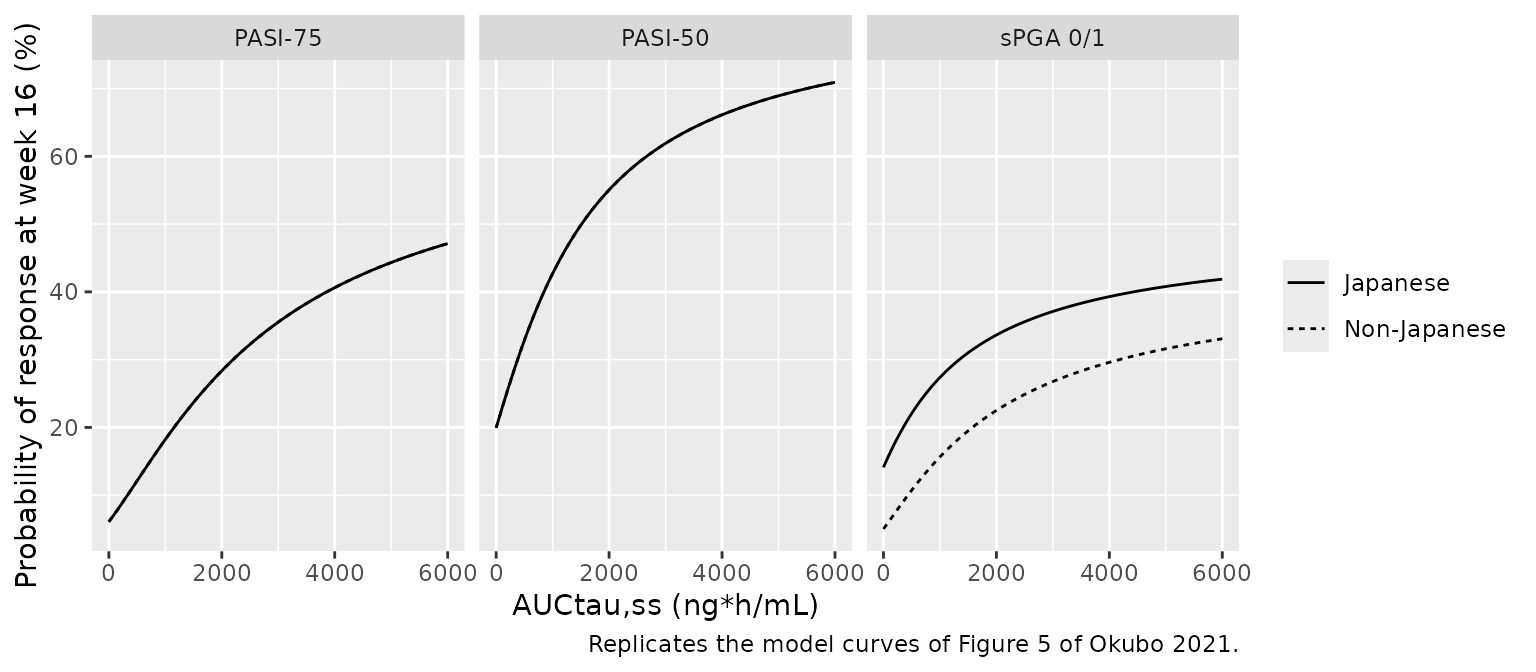
Figure S3: response over time
Typical-value time courses at the median non-Japanese AUC for each dose (Results 3.3), for comparison with the population predictions in Okubo 2021 Figure S3.
dose_auc <- tibble::tribble(
  ~regimen, ~AUC_APREMILAST,
  "Placebo", 0,
  "10 mg BID", 1065.4,
  "20 mg BID", 2030.6,
  "30 mg BID", 3169.2
)
figS3 <- tidyr::expand_grid(endpoint = names(er_models), dose_auc,
                            time = seq(0, 24, by = 0.5)) |>
  mutate(RACE_JAPANESE = 0L) |>
  group_by(endpoint) |>
  group_modify(function(d, k) {
    d$prob <- solve_er(k$endpoint, d |> mutate(id = row_number()) |>
                         select(id, time, AUC_APREMILAST, RACE_JAPANESE))
    d
  }) |>
  ungroup() |>
  mutate(endpoint = factor(endpoint, c("pasi75", "pasi50", "spga"),
                           c("PASI-75", "PASI-50", "sPGA 0/1")))
ggplot(figS3, aes(time, 100 * prob, colour = regimen)) +
  geom_line() +
  facet_wrap(~endpoint) +
  labs(x = "Time (weeks)", y = "Probability of response (%)", colour = NULL,
       caption = "Compare with Figure S3 of Okubo 2021 (population predictions).")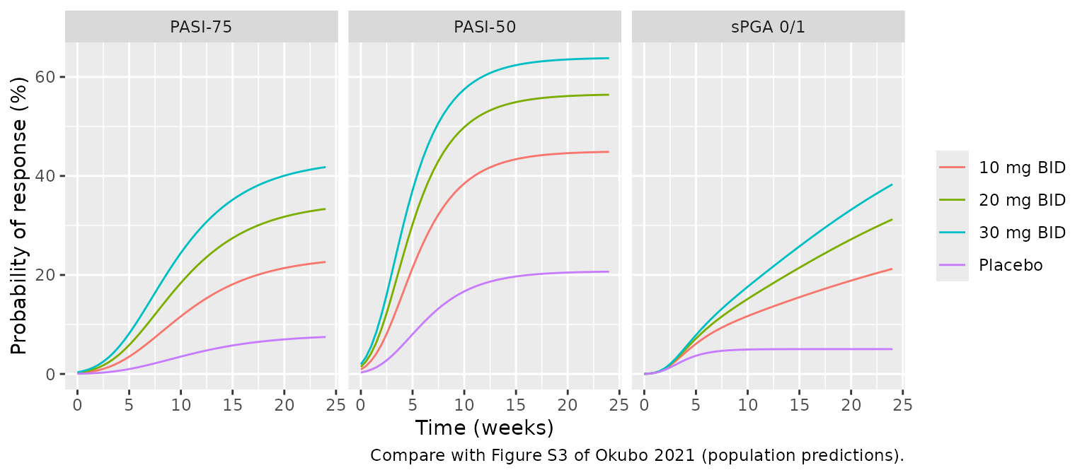
The sPGA curves rise steadily to week 24 rather than reaching their plateau by week 8 as the PASI curves do, which is the shape Figure S3C shows (30 mg twice daily: about 6% at week 4, 16% at week 8 and 40% at week 24).
PPK to E-R: arm-level week-16 response
Individual AUCtau,ss values from the virtual PK cohort (dose / CL) drive the three E-R models. The mean predicted probability per arm is shown next to the observed week-16 response rates the Discussion quotes for the 30 mg twice-daily arms; this is context, not a gate, because the observed rates come from single trials.
cohort_auc <- indiv |>
  mutate(AUC_APREMILAST = 1000 * dose_mg / cl,
         RACE_JAPANESE = as.integer(population == "Japanese"),
         time = 16)
arm_pred <- lapply(names(er_models), function(ep) {
  cohort_auc |>
    mutate(prob = solve_er(ep, cohort_auc |> select(id, time, AUC_APREMILAST, RACE_JAPANESE)),
           endpoint = ep)
}) |>
  bind_rows() |>
  group_by(treatment, endpoint) |>
  summarise(pred_pct = 100 * mean(prob), .groups = "drop") |>
  tidyr::pivot_wider(names_from = endpoint, values_from = pred_pct)
observed <- tibble::tribble(
  ~treatment, ~obs_pasi75, ~obs_spga,
  "Japanese 30 mg BID", 28.2, 29.6,
  "PSOR-005 30 mg BID", 40.9, 33.0,
  "ESTEEM 1 30 mg BID", 33.1, 21.7
)
arm_pred |>
  left_join(observed, by = "treatment") |>
  dplyr::rename(
    "Arm" = treatment,
    "PASI-75 model (%)" = pasi75, "PASI-50 model (%)" = pasi50,
    "sPGA model (%)" = spga, "PASI-75 observed (%)" = obs_pasi75,
    "sPGA observed (%)" = obs_spga
  ) |>
knitr::kable(digits = 1, caption = "Week-16 response: mean model prediction over the virtual cohort vs observed rates quoted in the Okubo 2021 Discussion.")| Arm | PASI-50 model (%) | PASI-75 model (%) | sPGA model (%) | PASI-75 observed (%) | sPGA observed (%) |
|---|---|---|---|---|---|
| ESTEEM 1 30 mg BID | 63.5 | 37.9 | 28.0 | 33.1 | 21.7 |
| Japanese 20 mg BID | 53.8 | 27.7 | 33.0 | NA | NA |
| Japanese 30 mg BID | 59.3 | 33.4 | 35.8 | 28.2 | 29.6 |
| PSOR-005 10 mg BID | 44.4 | 19.8 | 16.6 | NA | NA |
| PSOR-005 20 mg BID | 57.0 | 30.8 | 23.8 | NA | NA |
| PSOR-005 30 mg BID | 62.7 | 36.9 | 27.4 | 40.9 | 33.0 |
Assumptions and deviations
-
sPGA drug-effect onset rate (
lkdrug) is back-solved, not printed. Appendix S5 states that the sPGA E-R model has “an Emax-type effect model with an exponential delay component”, but Table S2 lists no rate for it. The maintainers back-solved it from the ten treated week-16 sPGA probabilities printed in Table S1 and Results 3.3. Every one of them requires the drug term to be 0.5784 of its full size at week 16 (rounding interval 0.5783-0.5786, across AUC values from 1065 to 3213ng*h/mLand both races), which with a first-order onset1 - exp(-kdrug t)giveskdrug = -log(1 - 0.5784) / 16 = 0.0540per week. Figure S3C supports the gradual onset; a constant scaling of the drug term by 0.58 would instead overpredict the early weeks (about 18% at week 4 for 30 mg) and underpredict week 24. The value happens to sit next to the printed K placebo of 0.579 per week; the maintainers treat that as a coincidence of digits, since a drug onset at 0.579 per week would be complete by week 16 and cannot reproduce Table S1. - PASI drug effect is undelayed. Appendix S5 says the PASI models have “a placebo parameter with an exponential delay term applied to the drug effect term”. Taken literally (the placebo onset also multiplying the drug term), the week-16 PASI-75 probability at 30 mg would be 33.9%, not the printed 36.5%. All 17 printed PASI-75 / PASI-50 probabilities are reproduced to rounding with the exponential onset on the placebo term only and the Emax drug term at full size, and this form also matches the early weeks of Figure S3A-B, so it is the form encoded.
- CL/F-Vc/F covariance not reported. The paper estimated a block variance on CL/F and Vc/F (Results 3.2) but Table 4 prints only the two variances, so the block is encoded as diagonal (correlation 0).
-
BSV scale. Table 4 prints between-subject
variability as a percentage; it is read as a CV and converted with
omega^2 = log(1 + CV^2). Reading it as100 * omegainstead would change the CL/F variance from 0.135 to 0.144 and the Ka variance from 0.528 to 0.696. - Fixed-zero random effects omitted. The lag time (Table 4) and every E-R parameter (Table S2) carried a between-subject variability fixed to 0; these are encoded without an eta. The E-R models therefore have no random effects, and their probabilities are typical-subject (population) predictions given the AUC.
-
Residual error of the E-R models. The source
likelihood is Bernoulli with no residual error; each E-R model carries a
placeholder additive residual (
addSd_prob_* = 0.001, held constant) so the nlmixr2 observation machinery accepts the model. It is not from the source. -
Disease reference category. The PPK model codes
disease as psoriasis, healthy or other (psoriatic or rheumatoid
arthritis in one phase 1 study), and only the psoriasis effect was
retained;
DIS_PSORIASIS = 0therefore covers both healthy and ‘other’ subjects. -
Sex coding. The paper codes male = 1 and prints a
1.25-fold CL/F for males. It is encoded on the canonical
SEXFase_sexm_cl^(1 - SEXF), so the 9.25 L/h typical value is the female value, as in the paper. - Subject count. Results 3.2 gives 517 subjects; the Table 4 caption prints n = 533. The population metadata uses 517, which is also the sum of the Table 3 study sizes.
- Virtual cohort. Age and body weight are normal with the Table 3 study means and CVs, truncated to 20-85 years and 40-180 kg; sex is Bernoulli with the Table 3 male fraction. Race, disease status and dose are set per arm. The paper’s E-R populations (Table 5: n = 89-613 per arm) are not reproduced in size.
- Errata. No correction notice for doi:10.1111/1346-8138.16068 was found in Europe PMC as of 2026-10-02.