Isatuximab with or without dexamethasone: M-protein and PFS (Thai 2023)
Source:vignettes/articles/Thai_2023_isatuximab.Rmd
Thai_2023_isatuximab.RmdModel and source
Thai 2023 developed a joint model of serum M-protein kinetics and progression-free survival (PFS) for single-agent isatuximab, with or without dexamethasone, in relapsed/refractory multiple myeloma (RRMM). It used the model to simulate the 10 and 20 mg/kg weekly-then-biweekly (qw-q2w) regimens, with and without dexamethasone, in Japanese patients, and so supported the Japanese approval of isatuximab +/- dexamethasone without an extra trial.
- Citation: Thai HT, Koiwai K, Shitara Y, Kazama H, Fau JB, Semiond D, Veyrat-Follet C. Model-based simulation to support the approval of isatuximab alone or with dexamethasone for the treatment of relapsed/refractory multiple myeloma in Japanese patients. CPT Pharmacometrics Syst Pharmacol. 2023;12(12):1846-1858. doi:10.1002/psp4.12947. Isatuximab PK layer: Fau JB et al. CPT Pharmacometrics Syst Pharmacol. 2020;9(11):649-658. doi:10.1002/psp4.12561.
- Article: https://doi.org/10.1002/psp4.12947 (open access; Appendix S1 holds the Monolix model code).
The model has four layers, all in one file because the authors fitted the M-protein and PFS parts jointly:
Isatuximab PK. The Fau 2020 two-compartment model with parallel time-varying linear and Michaelis-Menten elimination (also available on its own as
modellib("Fau_2020_isatuximab")). Thai 2023 used individual post-hoc PK parameters from it; here its population parameters and between-subject variability are embedded as fixed values, converted from hours to days.Dexamethasone K-PD. Dexamethasone concentrations were not measured, so doses enter a virtual compartment with a fixed elimination rate constant (2.42 /day) and volume (76.3 L).
-
Serum M-protein. A Claret tumor-growth-inhibition model:
where and are the isatuximab and dexamethasone molar concentrations (umol/L).
-
PFS. A log-logistic baseline hazard multiplied by baseline covariates and by the instantaneous M-protein slope:
Population
The model was fitted to 201 patients with RRMM and measurable serum M-protein from two single-agent isatuximab trials (Thai 2023 Tables 1-2): the multinational phase II NCT01084252 (n = 170; 3 mg/kg q2w to 20 mg/kg qw-q2w, 38 of them with weekly dexamethasone 40 mg) and the Japanese phase I/II NCT02812706 (n = 31; 10 or 20 mg/kg qw-q2w). Median age was 66 years (range 37-84), 46.3% were women, and median weight was 70 kg. Race was 70.6% White, 6.0% Black, 15.9% Asian. The median baseline serum M-protein was 28.1 g/L, albumin 35 g/L and beta-2-microglobulin 4.53 mg/L. IgG myeloma made up 69.2% and 15.4% had plasmacytomas. The analysis used 1774 serum M-protein observations (median 9 per patient).
str(rxode2::rxode(readModelDb("Thai_2023_isatuximab"))$population)
#> ℹ parameter labels from comments will be replaced by 'label()'
#> List of 14
#>  $ species       : chr "human"
#>  $ n_subjects    : int 201
#>  $ n_observations: int 1774
#>  $ n_studies     : int 2
#>  $ age_range     : chr "37-84 years"
#>  $ age_median    : chr "66 years"
#>  $ weight_range  : chr "37.6-153 kg"
#>  $ weight_median : chr "70.0 kg"
#>  $ sex_female_pct: num 46.3
#>  $ race_ethnicity: Named num [1:4] 70.6 6 15.9 7.5
#>   ..- attr(*, "names")= chr [1:4] "White" "Black" "Asian" "Other"
#>  $ disease_state : chr "Relapsed/refractory multiple myeloma with measurable serum M-protein (>= 2 serum M-protein values including bas"| __truncated__
#>  $ dose_range    : chr "Isatuximab IV 3 mg/kg q2w, 10 mg/kg q2w, 10 mg/kg q2w-q4w, 10 mg/kg qw-q2w or 20 mg/kg qw-q2w (qw-q2w = weekly "| __truncated__
#>  $ regions       : chr "Non-Japanese multinational phase II (NCT01084252, n = 170) and Japanese phase I/II (NCT02812706, n = 31)."
#>  $ notes         : chr "Baseline demographics from Thai 2023 Table 2 (median baseline B2M 4.53 mg/L, albumin 35 g/L, serum M-protein 28"| __truncated__
Source trace
| Equation / parameter | Value | Source location |
|---|---|---|
| M-protein ODE (Claret, Emax isatuximab + linear dexamethasone on shrinkage) | – | Methods equation; Appendix S1 mlxtran dM
|
| PFS log-logistic hazard with dM/dt link | – | Methods equations; Appendix S1 mlxtran haz
|
| Molar conversions, MW 150000 and 392.46 g/mol | – | Appendix S1 mlxtran CiM, CdM,
MW_ISA, MW_DEX
|
| Dexamethasone K-PD, KDEd = 2.42 /day, V = 76.3 L | fixed | Appendix S1 mlxtran KDEd, Cd=Ad/76.3
|
Isatuximab PK (lcl … etalkm) |
fixed | Fau 2020 Table S3, as in Fau_2020_isatuximab (Appendix
S1 ‘Pharmacokinetic model for isatuximab’) |
lrbase (M0) |
27 g/L | Table 3 |
e_nigg_rbase (beta1, non-IgG) |
-0.255 | Table 3 |
e_alb_rbase (beta2, ALBN) |
-1.83 | Table 3 |
e_alpr_rbase (beta3, ALKN) |
-0.233 | Table 3 |
e_lines_rbase (beta4, LINE) |
0.21 | Table 3 |
e_japan_rbase (beta5, Japanese study) |
-0.216 | Table 3 |
lp (KL) |
0.00531 /day | Table 3 |
e_nonrefractory_len_p (beta6, REF_Len = N) |
-0.514 | Table 3 |
lkkillmax (KD) |
0.0396 /day | Table 3 |
e_mcprot_kkillmax (beta7, MPROT) |
-0.56 | Table 3 |
llambda (R) |
0.0192 /day | Table 3 |
lec50 (EC50) |
1.13 umol/L (170 mg/L) | Table 3; Results text |
lslope_dexamethasone (k) |
5.47 L/umol | Table 3 |
etalrbase, etalp,
etalkkillmax, etallambda,
etalec50
|
omega 39.8, 94.7, 87, 113, 123% | Table 3 |
addSd, propSd
|
0.477 g/L, 7.21% | Table 3 |
llambda_pfs (Te) |
272 days | Table 3 |
lgamma_pfs (s) |
1.56 | Table 3 |
e_dexamethasone_pfs (beta8) |
-0.363 | Table 3 |
e_emd_pfs (beta9, PCYTOMA) |
0.799 | Table 3 |
e_b2m_pfs (beta10, B2MG) |
-1.76e-7 | Table 3 |
e_mprotein_slope_pfs (beta11, SlopeM) |
6.65 | Table 3 |
Simulation set-up
Isatuximab is given as 3-hour infusions on days 0, 7, 14 and 21, then
every 14 days. Dexamethasone is 40 mg weekly (20 mg for patients aged 75
or older), dosed into depot_kpd. Simulations run for 88
weeks with weekly M-protein observations.
mod <- readModelDb("Thai_2023_isatuximab")
tmax <- 616
isa_days <- c(0, 7, 14, 21, seq(28, tmax, by = 14))
obs_days <- seq(0, tmax, by = 7)

# One subject's events. dex_stop = Inf gives dexamethasone throughout;
# dex_stop = NA gives no dexamethasone.
make_events <- function(id, wt, mgkg, age, dex_stop) {
  isa <- data.frame(id = id, time = isa_days, amt = mgkg * wt, cmt = "central",
                    evid = 1, rate = mgkg * wt / 0.125)
  obs <- data.frame(id = id, time = obs_days, amt = NA_real_, cmt = "mprotein",
                    evid = 0, rate = NA_real_)
  out <- rbind(isa, obs)
  if (!is.na(dex_stop)) {
    dex_days <- seq(0, tmax - 1, by = 7)
    dex_days <- dex_days[dex_days < dex_stop]
    dex <- data.frame(id = id, time = dex_days, amt = ifelse(age >= 75, 20, 40),
                      cmt = "depot_kpd", evid = 1, rate = 0)
    out <- rbind(out, dex)
  }
  # The PFS dexamethasone indicator is 1 while the patient is on dexamethasone.
  out$CONMED_DEXAMETHASONE <- as.integer(!is.na(dex_stop) & out$time < dex_stop)
  out[order(out$time, -out$evid), ]
}
Typical-patient covariate effects (Figure S6)
Figure S6 of Thai 2023 shows the M-protein and PFS curves of a typical patient on isatuximab 20 mg/kg qw-q2w, varying one covariate at a time. The typical patient here has the Table 2 medians, IgG myeloma, no plasmacytoma, the non-Japanese study, lenalidomide-refractory disease and no dexamethasone; the two unreported centring values (ALKN, number of prior lines) are at their references.
typ_cov <- data.frame(WT = 70, B2M = 4.53, MM_NIGG = 0, ALB = 35, ALPR = 1,
  N_PRIOR_LINES = 4, REGION_JAPAN = 0, REFRACTORY_LEN = 1, MCPROT = 28.1,
  DIS_EMD = 0, FORM_ISA_P2F2 = 1, RACE_ASIAN = 0, SEXF = 0, AGE = 66)
scenarios <- list(
  "Typical"                  = list(),
  "Non-IgG MM"               = list(MM_NIGG = 1),
  "Not lenalidomide-refractory" = list(REFRACTORY_LEN = 0),
  "Albumin 25 g/L"           = list(ALB = 25),
  "Baseline M-protein 70 g/L" = list(MCPROT = 70),
  "Plasmacytoma"             = list(DIS_EMD = 1),
  "Dexamethasone"            = list(dex = TRUE)
)
typ <- bind_rows(lapply(names(scenarios), function(nm) {
  sc <- scenarios[[nm]]
  cv <- typ_cov
  for (v in setdiff(names(sc), "dex")) cv[[v]] <- sc[[v]]
  ev <- make_events(1, cv$WT, 20, cv$AGE, if (isTRUE(sc$dex)) Inf else NA)
  ev <- cbind(ev, cv[rep(1, nrow(ev)), ])
  s <- rxSolve(rxode2::zeroRe(mod), ev, returnType = "data.frame")
  s$scenario <- nm
  s
}))
#> ℹ parameter labels from comments will be replaced by 'label()'
#> ℹ omega/sigma items treated as zero: 'etalcl', 'etacl_time_max', 'etalcl_t50', 'etalcl_time_hill', 'etalvc', 'etalq', 'etalvp', 'etalvmax', 'etalkm', 'etalrbase', 'etalp', 'etalkkillmax', 'etallambda', 'etalec50'
#> ℹ parameter labels from comments will be replaced by 'label()'
#> ℹ omega/sigma items treated as zero: 'etalcl', 'etacl_time_max', 'etalcl_t50', 'etalcl_time_hill', 'etalvc', 'etalq', 'etalvp', 'etalvmax', 'etalkm', 'etalrbase', 'etalp', 'etalkkillmax', 'etallambda', 'etalec50'
#> ℹ parameter labels from comments will be replaced by 'label()'
#> ℹ omega/sigma items treated as zero: 'etalcl', 'etacl_time_max', 'etalcl_t50', 'etalcl_time_hill', 'etalvc', 'etalq', 'etalvp', 'etalvmax', 'etalkm', 'etalrbase', 'etalp', 'etalkkillmax', 'etallambda', 'etalec50'
#> ℹ parameter labels from comments will be replaced by 'label()'
#> ℹ omega/sigma items treated as zero: 'etalcl', 'etacl_time_max', 'etalcl_t50', 'etalcl_time_hill', 'etalvc', 'etalq', 'etalvp', 'etalvmax', 'etalkm', 'etalrbase', 'etalp', 'etalkkillmax', 'etallambda', 'etalec50'
#> ℹ parameter labels from comments will be replaced by 'label()'
#> ℹ omega/sigma items treated as zero: 'etalcl', 'etacl_time_max', 'etalcl_t50', 'etalcl_time_hill', 'etalvc', 'etalq', 'etalvp', 'etalvmax', 'etalkm', 'etalrbase', 'etalp', 'etalkkillmax', 'etallambda', 'etalec50'
#> ℹ parameter labels from comments will be replaced by 'label()'
#> ℹ omega/sigma items treated as zero: 'etalcl', 'etacl_time_max', 'etalcl_t50', 'etalcl_time_hill', 'etalvc', 'etalq', 'etalvp', 'etalvmax', 'etalkm', 'etalrbase', 'etalp', 'etalkkillmax', 'etallambda', 'etalec50'
#> ℹ parameter labels from comments will be replaced by 'label()'
#> ℹ omega/sigma items treated as zero: 'etalcl', 'etacl_time_max', 'etalcl_t50', 'etalcl_time_hill', 'etalvc', 'etalq', 'etalvp', 'etalvmax', 'etalkm', 'etalrbase', 'etalp', 'etalkkillmax', 'etallambda', 'etalec50'
typ <- typ |> distinct(scenario, time, .keep_all = TRUE)

ggplot(typ, aes(time / 7, mprotein, colour = scenario)) +
  geom_line() +
  labs(x = "Time (weeks)", y = "Serum M-protein (g/L)", colour = NULL,
       caption = "Replicates the M-protein panels of Figure S6 of Thai 2023.")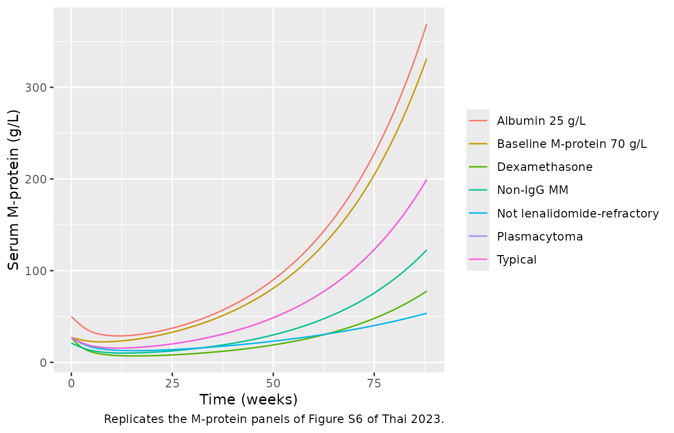
ggplot(typ, aes(time / 7, surv_pfs, colour = scenario)) +
  geom_line() +
  labs(x = "Time (weeks)", y = "PFS probability", colour = NULL,
       caption = "Replicates the PFS panels of Figure S6 of Thai 2023.")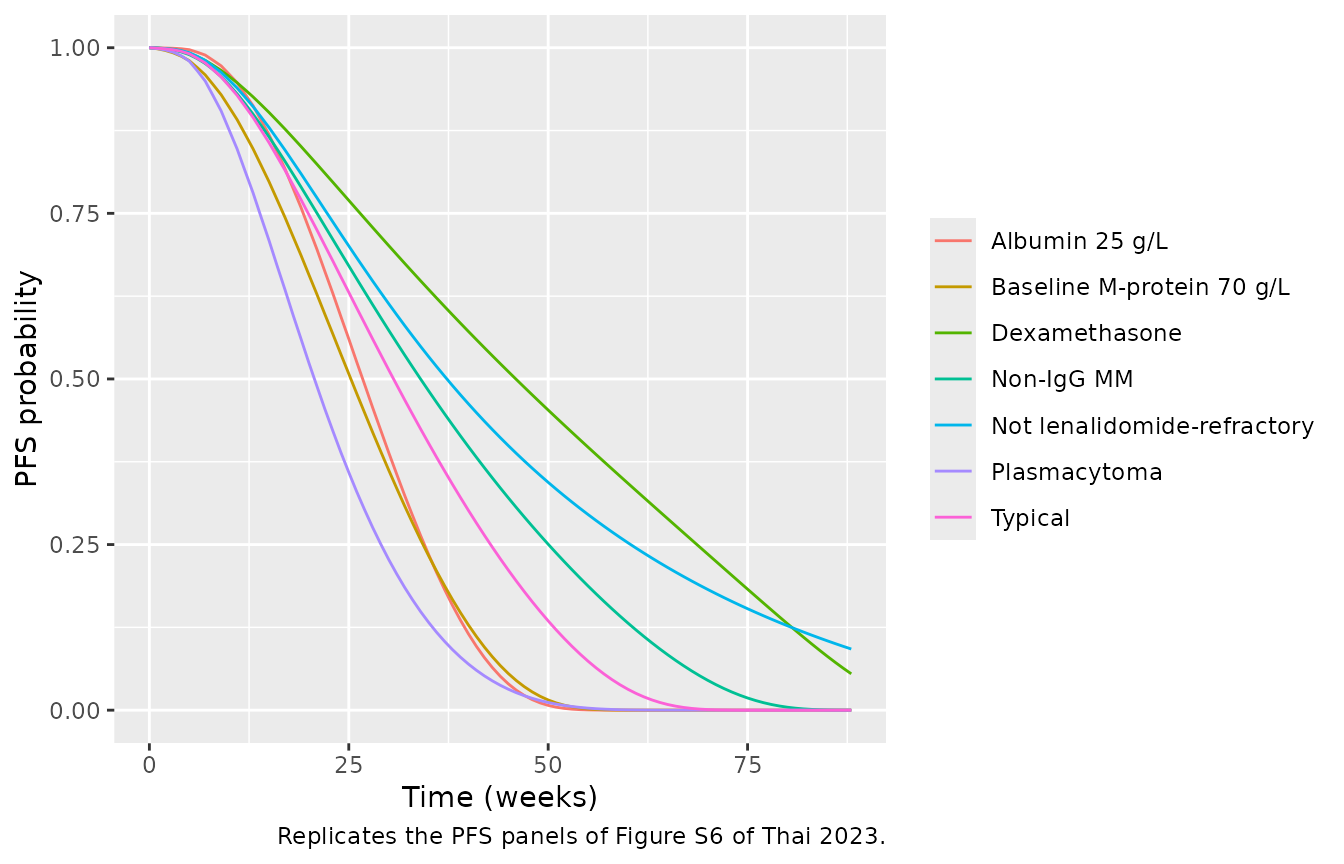
typ_sum <- typ |>
  group_by(scenario) |>
  summarise(
    m_80wk = mprotein[time == 560],
    median_pfs_wk = time[which(surv_pfs <= 0.5)[1]] / 7,
    .groups = "drop"
  ) |>
  mutate(ratio_to_typical = m_80wk / m_80wk[scenario == "Typical"])
typ_sum |>
  dplyr::rename("Scenario" = scenario, "M-protein at 80 weeks (g/L)" = m_80wk,
                "Median PFS (weeks)" = median_pfs_wk,
                "M-protein ratio to typical" = ratio_to_typical) |>
knitr::kable(digits = 2)| Scenario | M-protein at 80 weeks (g/L) | Median PFS (weeks) | M-protein ratio to typical |
|---|---|---|---|
| Albumin 25 g/L | 274.18 | 27 | 1.85 |
| Baseline M-protein 70 g/L | 246.37 | 26 | 1.66 |
| Dexamethasone | 57.67 | 46 | 0.39 |
| Non-IgG MM | 91.03 | 34 | 0.61 |
| Not lenalidomide-refractory | 44.83 | 38 | 0.30 |
| Plasmacytoma | 148.12 | 21 | 1.00 |
| Typical | 148.12 | 31 | 1.00 |
r <- setNames(typ_sum$ratio_to_typical, typ_sum$scenario)
stopifnot(
  # Figure S6: the not-refractory curve ends at about 65 g/L against about
  # 215 g/L (ratio ~0.30); the non-IgG curve at about 140 g/L (ratio ~0.65).
  # These are deterministic typical-value solves.
  r[["Not lenalidomide-refractory"]] > 0.2, r[["Not lenalidomide-refractory"]] < 0.4,
  r[["Non-IgG MM"]] > 0.5, r[["Non-IgG MM"]] < 0.75,
  # Figure S6: the typical PFS curve crosses 0.5 at roughly 30 weeks.
  typ_sum$median_pfs_wk[typ_sum$scenario == "Typical"] > 25,
  typ_sum$median_pfs_wk[typ_sum$scenario == "Typical"] < 36
)
The covariate contrasts match Figure S6 closely. The covariates on M0 (IgG type, albumin, ALKN, prior lines, Japanese study) scale the whole M-protein curve, because the ODE is linear in M. The non-IgG contrast is stronger than exp(-0.255) = 0.775 because non-IgG myeloma also lowers isatuximab clearance in the Fau 2020 PK layer. The typical curve itself regrows more slowly than Figure S6 (about 150 g/L at 80 weeks against about 215 g/L; see Assumptions and deviations).
Virtual cohort
Two hundred virtual patients are drawn to resemble Table 2. Each regimen is simulated in the same patients with the same random effects, so the arms differ only by treatment.
set.seed(2023)
n <- 200
rtrunc_lnorm <- function(n, med, sdlog, lo, hi) pmin(pmax(exp(rnorm(n, log(med), sdlog)), lo), hi)
cohort <- data.frame(
  id = seq_len(n),
  WT = rtrunc_lnorm(n, 70, 0.2, 37.6, 153),
  AGE = pmin(pmax(rnorm(n, 66, 9), 37), 84),
  B2M = rtrunc_lnorm(n, 4.53, 0.6, 1.32, 19.5),
  ALB = pmin(pmax(rnorm(n, 35, 5), 18), 48),
  ALPR = rtrunc_lnorm(n, 1, 0.4, 0.2, 5),
  N_PRIOR_LINES = pmin(pmax(round(rtrunc_lnorm(n, 4, 0.45, 1, 11)), 1), 11),
  REGION_JAPAN = rbinom(n, 1, 31 / 201),
  REFRACTORY_LEN = rbinom(n, 1, 0.85),
  MCPROT = rtrunc_lnorm(n, 28.1, 0.6, 6, 84),
  MM_NIGG = rbinom(n, 1, 62 / 201),
  DIS_EMD = rbinom(n, 1, 0.154),
  SEXF = rbinom(n, 1, 0.463),
  FORM_ISA_P2F2 = 1
)
cohort$RACE_ASIAN <- cohort$REGION_JAPAN

arms <- tibble::tribble(
  ~arm,                       ~mgkg, ~dex_stop,
  "Isa 10 mg/kg qw-q2w",      10,    NA,
  "Isa 20 mg/kg qw-q2w",      20,    NA,
  "Isa 20 mg/kg qw-q2w + Dex", 20,   Inf,
  "Isa 20 mg/kg + Dex 0-3M",  20,    84,
  "Isa 20 mg/kg + Dex 0-6M",  20,    168
)

sim_arm <- function(mgkg, dex_stop) {
  ev <- bind_rows(lapply(seq_len(n), function(i) {
    make_events(i, cohort$WT[i], mgkg, cohort$AGE[i], dex_stop)
  }))
  ev <- left_join(ev, select(cohort, -AGE), by = "id")
  rxode2::rxSetSeed(20231)
  rxSolve(mod, ev, returnType = "data.frame")
}
sims <- bind_rows(lapply(seq_len(nrow(arms)), function(k) {
  s <- sim_arm(arms$mgkg[k], arms$dex_stop[k])
  s$arm <- arms$arm[k]
  s
})) |>
  distinct(arm, id, time, .keep_all = TRUE)
#> ℹ parameter labels from comments will be replaced by 'label()'
Change in serum M-protein at week 8 (Figures 2a and 3a)
wk8 <- sims |>
  filter(time %in% c(0, 56)) |>
  select(arm, id, time, mprotein) |>
  pivot_wider(names_from = time, values_from = mprotein, names_prefix = "t") |>
  mutate(pct_change = 100 * (t56 / t0 - 1)) |>
  left_join(select(cohort, id, REGION_JAPAN), by = "id")

wk8 |>
  filter(arm %in% arms$arm[1:3]) |>
  ggplot(aes(arm, pmin(pct_change, 100))) +
  geom_boxplot(outlier.shape = NA) +
  coord_cartesian(ylim = c(-100, 100)) +
  labs(x = NULL, y = "Change from baseline in serum M-protein at week 8 (%)",
       caption = "Replicates Figures 2a and 3a of Thai 2023 (all patients).")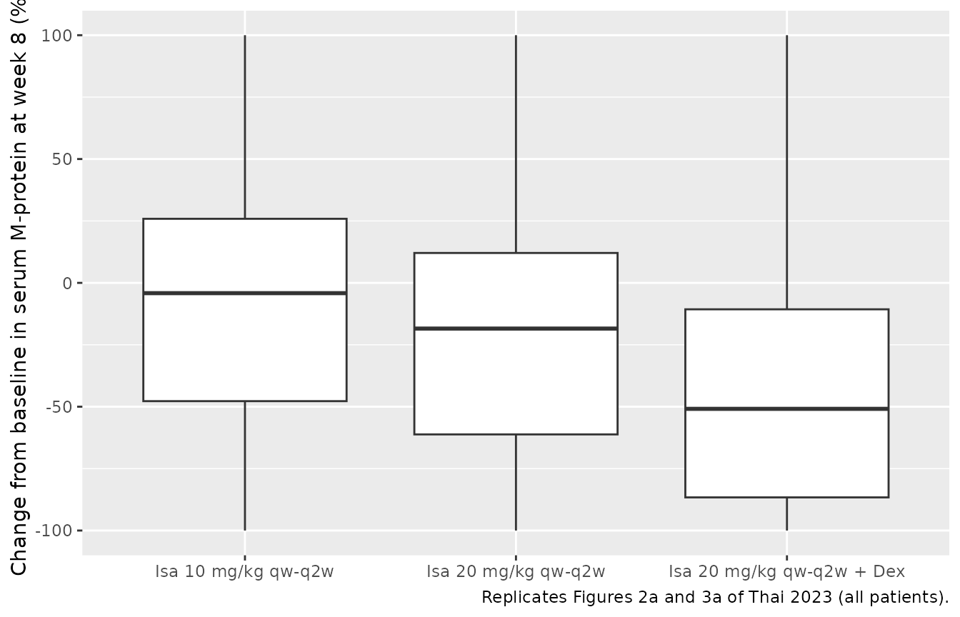
PFS (Figures 2b and 3c, Table 4)
The population PFS curve is the mean of the individual survival curves.
pfs <- sims |>
  group_by(arm, time) |>
  summarise(surv = mean(surv_pfs), .groups = "drop")

pfs |>
  filter(arm %in% arms$arm[1:3]) |>
  ggplot(aes(time / 7, surv, colour = arm)) +
  geom_line() +
  labs(x = "Time (weeks)", y = "PFS probability", colour = NULL,
       caption = "Replicates Figures 2b and 3c of Thai 2023 (all patients).")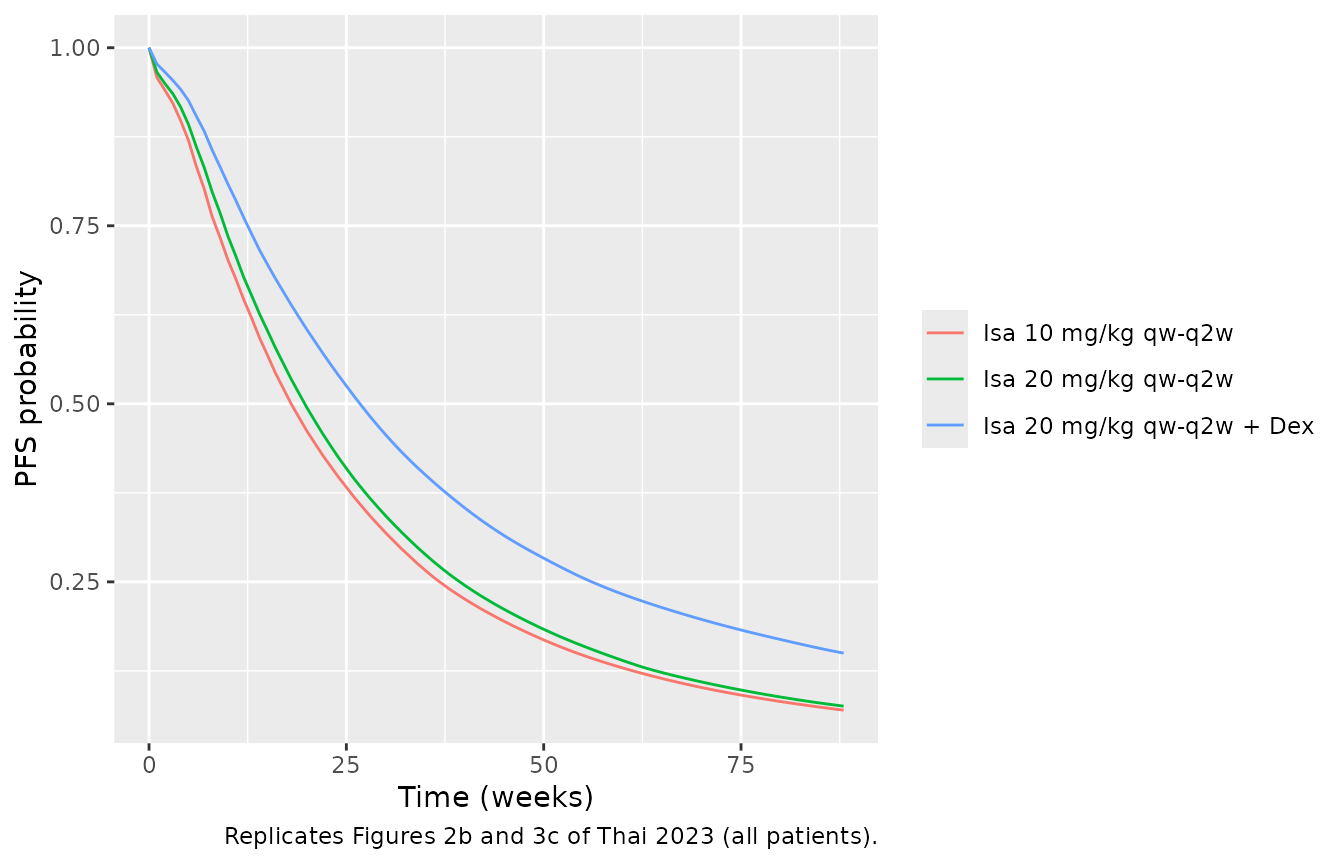
median_pfs <- function(time, surv) time[which(surv <= 0.5)[1]] / 7
pfs_med <- pfs |>
  group_by(arm) |>
  summarise(median_pfs_wk = median_pfs(time, surv), .groups = "drop")
Comparison with the published simulations
published <- tibble::tribble(
  ~arm,                       ~pub_wk8, ~pub_pfs,
  "Isa 10 mg/kg qw-q2w",      -22,      19.3 - 2.4,
  "Isa 20 mg/kg qw-q2w",      -30,      19.3,
  "Isa 20 mg/kg qw-q2w + Dex", -54,     25.6,
  "Isa 20 mg/kg + Dex 0-3M",  NA,       20.9,
  "Isa 20 mg/kg + Dex 0-6M",  NA,       21.3
)
cmp <- wk8 |>
  group_by(arm) |>
  summarise(sim_wk8 = median(pct_change), .groups = "drop") |>
  left_join(pfs_med, by = "arm") |>
  left_join(published, by = "arm") |>
  mutate(arm = factor(arm, levels = arms$arm)) |>
  arrange(arm)
cmp |>
  dplyr::rename("Regimen (all patients)" = arm,
                "Week-8 M-protein change, simulated (median %)" = sim_wk8,
                "Week-8 M-protein change, Thai 2023 (median %)" = pub_wk8,
                "Median PFS, simulated (weeks)" = median_pfs_wk,
                "Median PFS, Thai 2023 (weeks)" = pub_pfs) |>
knitr::kable(digits = 1)| Regimen (all patients) | Week-8 M-protein change, simulated (median %) | Median PFS, simulated (weeks) | Week-8 M-protein change, Thai 2023 (median %) | Median PFS, Thai 2023 (weeks) |
|---|---|---|---|---|
| Isa 10 mg/kg qw-q2w | -4.2 | 19 | -22 | 16.9 |
| Isa 20 mg/kg qw-q2w | -18.5 | 20 | -30 | 19.3 |
| Isa 20 mg/kg qw-q2w + Dex | -50.9 | 27 | -54 | 25.6 |
| Isa 20 mg/kg + Dex 0-3M | -50.9 | 23 | NA | 20.9 |
| Isa 20 mg/kg + Dex 0-6M | -50.9 | 26 | NA | 21.3 |
Published values: week-8 changes from the Results text (Figures 2a and 3a); median PFS from Table 4. The 10 mg/kg median PFS is the 20 mg/kg value minus the reported 2.4-week gain.
paired <- wk8 |>
  select(arm, id, pct_change) |>
  pivot_wider(names_from = arm, values_from = pct_change)
pfs_of <- function(a) cmp$median_pfs_wk[cmp$arm == a]
stopifnot(
  # Structural: monotherapy median PFS near the published 19.3 weeks.
  abs(pfs_of("Isa 20 mg/kg qw-q2w") - 19.3) < 5,
  # Dexamethasone prolongs PFS, and full-duration dexamethasone more than
  # 3 months of it.
  pfs_of("Isa 20 mg/kg qw-q2w + Dex") > pfs_of("Isa 20 mg/kg qw-q2w"),
  pfs_of("Isa 20 mg/kg qw-q2w + Dex") >= pfs_of("Isa 20 mg/kg + Dex 0-3M"),
  # Paired within patient (same random effects): the higher dose and the
  # added dexamethasone lower week-8 M-protein for the median patient.
  median(paired[["Isa 20 mg/kg qw-q2w"]] - paired[["Isa 10 mg/kg qw-q2w"]]) < 0,
  median(paired[["Isa 20 mg/kg qw-q2w + Dex"]] - paired[["Isa 20 mg/kg qw-q2w"]]) < 0
)
Median PFS is close to Table 4 for isatuximab 20 mg/kg alone (about 20 against 19.3 weeks) and with dexamethasone (about 27 against 25.6 weeks), and the week-8 decrease with dexamethasone is close to the published 54%. The week-8 decrease on isatuximab alone is smaller than published (about 18% against 30% at 20 mg/kg, and about 4% against 22% at 10 mg/kg), and the short-duration dexamethasone arms keep more of the full-duration PFS gain than Table 4 reports. The virtual cohort draws covariates that the paper does not report (lenalidomide-refractory fraction, number of prior lines, ALKN), uses population rather than individual PK, and reads the between-subject variability as Monolix standard deviations (see Assumptions and deviations), so these centres can move by several percentage points or weeks.
Japanese patients (Figure 3b and 3d)
wk8 |>
  filter(REGION_JAPAN == 1, arm %in% arms$arm[2:3]) |>
  group_by(arm) |>
  summarise(n = n(), median_wk8_change = median(pct_change), .groups = "drop") |>
  dplyr::rename("Regimen (Japanese patients)" = arm, "N" = n,
                "Week-8 M-protein change (median %)" = median_wk8_change) |>
knitr::kable(digits = 1)| Regimen (Japanese patients) | N | Week-8 M-protein change (median %) |
|---|---|---|
| Isa 20 mg/kg qw-q2w | 31 | -31.7 |
| Isa 20 mg/kg qw-q2w + Dex | 31 | -62.3 |
Thai 2023 reports medians of -43% (isatuximab alone) and -67% (with dexamethasone) in Japanese patients. The virtual Japanese subgroup shows a smaller decrease on isatuximab alone (about -32%) and a similar one with dexamethasone (about -62%); with about 30 Japanese patients these medians are imprecise.
Isatuximab exposure (PKNCA)
Thai 2023 reports no NCA. As a check on the embedded PK layer, PKNCA computes the first-week Cmax and AUC of the typical patient at each dose.
nca_typ <- bind_rows(lapply(c(10, 20), function(d) {
  ev <- et(amt = d * 70, time = 0, cmt = "central", rate = d * 70 / 0.125) |>
    et(seq(0, 7, by = 0.125), cmt = "central")
  ev <- cbind(as.data.frame(ev), typ_cov[rep(1, nrow(as.data.frame(ev))), ])
  ev$CONMED_DEXAMETHASONE <- 0
  s <- rxSolve(rxode2::zeroRe(mod), ev, returnType = "data.frame")
  s$treatment <- paste(d, "mg/kg")
  s$id <- 1
  s
}))
#> ℹ parameter labels from comments will be replaced by 'label()'
#> ℹ omega/sigma items treated as zero: 'etalcl', 'etacl_time_max', 'etalcl_t50', 'etalcl_time_hill', 'etalvc', 'etalq', 'etalvp', 'etalvmax', 'etalkm', 'etalrbase', 'etalp', 'etalkkillmax', 'etallambda', 'etalec50'
#> ℹ parameter labels from comments will be replaced by 'label()'
#> ℹ omega/sigma items treated as zero: 'etalcl', 'etacl_time_max', 'etalcl_t50', 'etalcl_time_hill', 'etalvc', 'etalq', 'etalvp', 'etalvmax', 'etalkm', 'etalrbase', 'etalp', 'etalkkillmax', 'etallambda', 'etalec50'
conc <- nca_typ |>
  filter(!is.na(Cc)) |>
  distinct(treatment, time, .keep_all = TRUE) |>
  select(id, treatment, time, Cc)
dose <- data.frame(id = 1, treatment = c("10 mg/kg", "20 mg/kg"), time = 0,
                   amt = c(700, 1400))
pc <- PKNCAconc(conc, Cc ~ time | treatment + id)
pd <- PKNCAdose(dose, amt ~ time | treatment + id)
intervals <- data.frame(start = 0, end = 7, cmax = TRUE, auclast = TRUE)
nca <- pk.nca(PKNCAdata(pc, pd, intervals = intervals))
nca_tab <- as.data.frame(nca$result) |>
  filter(PPTESTCD %in% c("cmax", "auclast")) |>
  select(treatment, PPTESTCD, PPORRES) |>
  pivot_wider(names_from = PPTESTCD, values_from = PPORRES)
nca_tab |>
  dplyr::rename("Dose" = treatment, "Cmax (mg/L)" = cmax,
                "AUC0-7 days (mg*day/L)" = auclast) |>
knitr::kable(digits = 1)| Dose | AUC0-7 days (mg*day/L) | Cmax (mg/L) |
|---|---|---|
| 10 mg/kg | 533.8 | 158.6 |
| 20 mg/kg | 1116.1 | 317.5 |
Assumptions and deviations
-
Covariate form. The paper prints no covariate
equations. Monolix log-normal parameters with continuous covariates are
encoded as
log(P) = log(Ppop) + beta * log(cov / reference). Figure S6 supports this: a linear MPROT term of -0.56 per g/L would remove almost all drug effect at high baseline M-protein, and the albumin P5 curve starts near 50 g/L, which matches (25/35)^-1.83 = 1.85 times 27 g/L. References are the Table 2 medians (albumin 35 g/L, baseline M-protein 28.1 g/L, B2M 4.53 mg/L). Albumin normalised to the upper limit of normal (ALBN) is entered as absolute albumin, since the ULN cancels in the ratio to the median. -
Unreported centring values. The medians of ALKN
(alkaline phosphatase / ULN) and of the number of prior lines are not
reported. The model centres ALKN on the ULN (
ALPR = 1) and prior lines on 4. A typical patient whose true medians differ two-fold would have M0 off by about 17%. -
New covariate columns. The maintainers registered
ALPR(alkaline phosphatase / ULN),N_PRIOR_LINES(continuous count of prior lines) andREFRACTORY_LEN(1 = lenalidomide-refractory). The paper’s effect is on ‘REF_Len = N’, so the model applies it as(1 - REFRACTORY_LEN). - Between-subject variability. Monolix reports omega as the standard deviation of the random effect; Table 3’s ‘Interindividual variability (%)’ is read as 100 * omega and squared (for example 1.23^2 = 1.51 for EC50). If the column were instead a CV, the variances would be log(1 + CV^2) (0.92 for EC50). Only the spread of individual curves depends on this choice, not the typical values. In the virtual cohort the CV reading moved the monotherapy week-8 median from about -18% to about -25% and the median PFS by about 2 weeks, so the published simulations do not settle it.
-
Residual error. Monolix’s default combined error
model
a + b*fis encoded withcombined1(). - Isatuximab PK. Thai 2023 drove the model with individual post-hoc PK parameters (typical values for 4 patients without PK). Here the Fau 2020 population model is embedded with its covariates and variability fixed. The Japanese trial was later found to have lower isatuximab clearance in a pooled PK analysis that is not reproduced here, so the Japanese-patient simulations use the Fau 2020 covariates only (Asian race on Vc).
-
Convention check.
checkModelConventions()warns thatcl_time_maxis not log-transformed. It is carried over unchanged fromFau_2020_isatuximab: CLm is a signed log-ratio with a normally distributed random effect, so a log transform would not fit. -
Hazard start time. The Monolix code switches the
hazard on at a per-patient time
Tstart, whose values are not given. The hazard here runs from the first dose. -
Numerical cap on the hazard. The log of the hazard
multiplier is capped at 50. When simulated M-protein regrows at several
g/L per day,
6.65 * dM/dtoverflowsexp(); at the cap, survival is already zero, so the cap only preventsInf/NaNvalues. -
B2M effect on PFS. beta10 = -1.76e-7 is negligible
under either a log or a linear covariate form (Thai 2023 describe it as
“extremely low”). It is encoded as
log(B2M / 4.53)for consistency. - Dexamethasone indicator. The PFS covariate ‘Dex = Y’ is the randomised arm. In the short-duration scenarios it is switched off when dexamethasone stops; the paper does not say how it handled this.
- Typical curve versus Figure S6. The typical patient’s M-protein falls to about 16 g/L at week 11 and reaches about 150 g/L at week 80, whereas Figure S6 shows a shallower nadir and about 215 g/L. The covariate contrasts and the typical median PFS (about 30 weeks) match the figure. The cause of the gap was not found; the figure’s typical patient may use different PK or covariate values from those assumed here.
- Table 2 typo. The ‘All’ column prints 31 (15.4%) non-IgG patients, a copy of the plasmacytoma row; the per-trial counts (56 + 6 = 62, 30.8%) are used.
- Virtual-cohort covariates not reported in the paper. The lenalidomide-refractory fraction (85%), the spread of ALKN and prior lines, and age are assumptions. Infusion duration (3 hours) is also assumed.
- No erratum to Thai 2023 was found (checked 2026-11-07).