Vestronidase alfa (Qi 2019)
Source:vignettes/articles/Qi_2019_vestronidaseAlfa.Rmd
Qi_2019_vestronidaseAlfa.RmdModel and source
mod <- readModelDb("Qi_2019_vestronidaseAlfa")
ui <- rxode2::rxode(mod)
#> ℹ parameter labels from comments will be replaced by 'label()'- Citation: Qi Y, McKeever K, Taylor J, Haller C, Song W, Jones SA, Shi J. Pharmacokinetic and Pharmacodynamic Modeling to Optimize the Dose of Vestronidase Alfa, an Enzyme Replacement Therapy for Treatment of Patients with Mucopolysaccharidosis Type VII: Results from Three Trials. Clin Pharmacokinet. 2019;58(5):673-683. doi:10.1007/s40262-018-0721-y. Erratum: Clin Pharmacokinet. 2019;58(5):685. doi:10.1007/s40262-018-0726-6 (corrects a ClinicalTrials.gov identifier in the Introduction; no parameter value is affected).
- Article: https://doi.org/10.1007/s40262-018-0721-y
- Erratum: https://doi.org/10.1007/s40262-018-0726-6
- Full text (open access): https://www.ncbi.nlm.nih.gov/pmc/articles/PMC6451706/
Vestronidase alfa (UX003) is a recombinant human beta-glucuronidase enzyme replacement therapy for mucopolysaccharidosis type VII (MPS VII, Sly syndrome). Qi 2019 pooled three trials to build a two-compartment population PK model and a sequential inhibitory-Imax exposure-response model for urinary glycosaminoglycan (uGAG) reduction, and used them to justify the approved 4 mg/kg every-other-week (QOW) regimen.
Population
The analysis pooled 23 subjects with MPS VII from three trials (Qi 2019 Table 1): 3 subjects from a phase I/II dose-titration study (NCT01856218, 1-4 mg/kg QOW), 8 subjects under 5 years of age from a phase II study (NCT02418455, 4 mg/kg QOW), and 12 subjects from a phase III blind-start placebo-controlled study (NCT02230566, 4 mg/kg QOW). Ages ranged from 1.7 to 25.3 years (median 10.1) and baseline body weights from 9.41 to 104.0 kg (median 24.8, mean 37.7). The cohort was 52% female and 61% White / 22% Other / 13% Asian / 4% Black. Fifteen subjects contributed intensively sampled PK profiles and eight contributed sparse profiles. All doses were given as approximately 4-hour intravenous infusions in which the first 2.5% of the total volume was infused over the first hour.
The same metadata is available programmatically:
str(ui$population)
#> List of 14
#>  $ species       : chr "human"
#>  $ n_subjects    : int 23
#>  $ n_studies     : int 3
#>  $ age_range     : chr "1.7-25.3 years"
#>  $ age_median    : chr "10.1 years (mean 11.0, SD 7.7)"
#>  $ weight_range  : chr "9.41-104.0 kg"
#>  $ weight_median : chr "24.8 kg (mean 37.7, SD 27.7)"
#>  $ sex_female_pct: num 52
#>  $ race_ethnicity: Named num [1:4] 61 13 4 22
#>   ..- attr(*, "names")= chr [1:4] "White" "Asian" "Black" "Other"
#>  $ disease_state : chr "Mucopolysaccharidosis type VII (MPS VII, Sly syndrome), an ultra-rare lysosomal storage disorder caused by beta"| __truncated__
#>  $ dose_range    : chr "Vestronidase alfa 1, 2, or 4 mg/kg by intravenous infusion every other week (QOW), infused over approximately 4"| __truncated__
#>  $ regions       : chr "Multinational (three clinical trials: NCT01856218, NCT02418455, NCT02230566)."
#>  $ sampling      : chr "15 subjects contributed intensively sampled PK profiles and 8 contributed sparse profiles (Qi 2019 Results). Ur"| __truncated__
#>  $ notes         : chr "Demographics from Qi 2019 Table 1 (overall column across the three studies: study 1 phase I/II, n = 3, ages 5.5"| __truncated__
Source trace
Every ini() entry carries an in-file comment naming its
source location in
inst/modeldb/specificDrugs/Qi_2019_vestronidaseAlfa.R. They
are collected here for review.
| Equation / parameter | Value | Source location |
|---|---|---|
lcl (CL) |
1.97 L/h | Table 2, point estimate (RSE 9.61%) |
lvc (Vc) |
1.52 L | Table 2, point estimate (RSE 9.64%) |
lq (Q) |
0.931 L/h | Table 2, point estimate (RSE 16.3%) |
lvp (Vp) |
3.11 L | Table 2, point estimate (RSE 4.23%) |
e_wt_cl_q |
0.587 | Table 2, “BWT on CL and Q” (RSE 12.4%) |
e_wt_vc_vp |
0.483 | Table 2, “BWT on Vc and Vp” (RSE 17.7%) |
| Reference weight 20 kg | n/a | Table 2 footnote b (“Centered on a body weight of 20 kg”) |
| Exponents estimated, not fixed | n/a | Table 2 footnote c (CIs exclude 0.75 / 1) |
etalcl, etalvc, etalq,
etalvp
|
0.170, 0.0944, 0.563, 0.0236 | Table 2, omega^2 column (reported directly) |
propSd |
sqrt(0.109) = 0.330 | Table 2, sigma^2 proportional = 0.109 (CV 33.0%) |
IIV model theta_i = theta_TV * exp(eta_i)
|
n/a | Methods, Population PK Modeling, first displayed equation |
Residual model DV = IPRED * (1 + eps)
|
n/a | Methods, Population PK Modeling, second displayed equation |
rbase_ucs, rbase_uds (I0) |
fixed at 0 | Methods, Exposure-Response Analysis (“I0 is the no-drug response and fixed to 0”) |
limax_ucs / limax_uds
|
82.0% / 76.9% | Table 4, Imax row |
lic50_ucs / lic50_uds
|
8.6 / 7.3 ug*h/mL | Table 4, IC50 row |
etalimax_ucs / etalimax_uds
|
7.9% / 8.7% CV | Table 4, IIV for Imax row |
addSd_uCSchange / addSd_uDSchange
|
6.1 / 6.4 | Table 4, additive residual error row |
I = I0 - Imax * AUC / (AUC + IC50) |
n/a | Methods, Exposure-Response Analysis, displayed equation |
Two transcription points are worth stating explicitly because both are easy to get wrong from a secondary source.
The omega values are variances, transcribed
directly. Table 2 reports omega^2 in its own
column, so no back-transformation from the CV% column is performed. That
matters here: Table 2 footnote d declares that the CV% column
uses CV = sqrt(exp(omega^2) - 1) only when
omega^2 > 0.15, and a plain
sqrt(omega^2) below that threshold. The column therefore
switches formula row by row (log-normal for CL and Q, plain SD for Vc
and Vp), and inverting it with a single formula would misstate the Vc
and Vp variances by a few percent.
The exposure-response equation carries a leading minus
sign. The displayed equation is
I = I0 - Imax * AUC / (AUC + IC50), verified against the
JATS MathML of the source XML. With I0 fixed at 0,
I is the percent change from baseline and is
therefore negative, which is what the Figure 4 axis (“% Change from
baseline”) shows.
Structural identities
These checks are deterministic: they compare the packaged model against quantities the paper derives from the very same parameters, so any disagreement is a transcription error rather than simulation noise. They are gated tightly.
# Typical values at the 20 kg reference weight, read back out of the model.
th <- setNames(ui$theta, names(ui$theta))
CL <- exp(th[["lcl"]]); Vc <- exp(th[["lvc"]])
Q  <- exp(th[["lq"]]);  Vp <- exp(th[["lvp"]])

# Terminal disposition half-life of a two-compartment model.
k10 <- CL / Vc; k12 <- Q / Vc; k21 <- Q / Vp
a <- k10 + k12 + k21
lambda_z <- (a - sqrt(a^2 - 4 * k10 * k21)) / 2
thalf <- log(2) / lambda_z

# Weight-normalised CL and Vss at the cohort median weight (24.8 kg). The paper
# normalises the 20 kg typical values by the median weight WITHOUT re-applying
# the allometric exponents -- see the note below.
wt_median <- 24.8
cl_per_kg  <- CL / wt_median
vss_per_kg <- (Vc + Vp) / wt_median

ident <- tibble::tibble(
  Quantity = c("Terminal half-life (h)",
               "CL normalised by median weight (L/h/kg)",
               "Vss = Vc + Vp normalised by median weight (L/kg)"),
  Model    = c(thalf, cl_per_kg, vss_per_kg),
  Published = c(3.6, 0.079, 0.19),
  Source   = c("Results, Population PK", "Results, Population PK", "Results, Population PK")
) |>
  mutate(`% diff` = 100 * (Model - Published) / Published)

knitr::kable(ident, digits = 3,
caption = "Model-internal identities against the values Qi 2019 derives from the same parameters.")| Quantity | Model | Published | Source | % diff |
|---|---|---|---|---|
| Terminal half-life (h) | 3.601 | 3.600 | Results, Population PK | 0.017 |
| CL normalised by median weight (L/h/kg) | 0.079 | 0.079 | Results, Population PK | 0.551 |
| Vss = Vc + Vp normalised by median weight (L/kg) | 0.187 | 0.190 | Results, Population PK | -1.740 |
stopifnot(
  abs(thalf - 3.6) / 3.6 < 0.01,          # paper rounds to 3.6 h; model gives 3.601
  abs(cl_per_kg - 0.079) / 0.079 < 0.01,
  abs(vss_per_kg - 0.19) / 0.19 < 0.02
)
Note that the paper’s per-kilogram values are the 20 kg typical values divided by the median weight, not allometrically rescaled to 24.8 kg. Rescaling would give CL = 1.97 * (24.8/20)^0.587 = 2.235 L/h, i.e. 0.0901 L/h/kg. The identity above reproduces the paper’s own arithmetic, and the allometric value is used everywhere a profile is actually simulated.
Event tables
Vestronidase alfa is infused over approximately 4 hours with the first 2.5% of the volume delivered in the first hour, so every dose is a two-rate infusion.
# Two-rate 4-hour infusion: 2.5% of the dose over hour 1, 97.5% over hours 1-4.
qi_dose_rows <- function(id, dose_mg, start_times, wt) {
  n <- length(start_times)
  tibble::tibble(
    # Interleave the two rate segments of each infusion: t0, t0 + 1 h.
    time = as.vector(rbind(start_times, start_times + 1)),
    amt  = rep(c(0.025 * dose_mg, 0.975 * dose_mg), times = n),
    rate = rep(c(0.025 * dose_mg / 1, 0.975 * dose_mg / 3), times = n),
    id = id, evid = 1L, cmt = "central", dvid = NA_integer_, WT = wt
  ) |>
    dplyr::select(id, time, amt, rate, evid, cmt, dvid, WT)
}

# Observation rows. The model declares three endpoints (Cc, uCSchange,
# uDSchange), so rxode2 requires each observation record to identify its
# endpoint. `dvid = 1L` selects Cc; every algebraic observable is still returned
# as a column, so one dvid = 1L grid yields the PK and both PD outputs.
qi_obs_rows <- function(id, times, wt) {
  tidyr::expand_grid(id = id, time = times) |>
    dplyr::transmute(id, time, amt = NA_real_, rate = NA_real_, evid = 0L,
                     cmt = NA_character_, dvid = 1L, WT = wt)
}

qi_solve <- function(events, ..., typical = TRUE) {
  args <- list(mod, as.data.frame(events), returnType = "data.frame",
               # rxode2's ODE->linCmt auto-conversion corrupts the dvid->cmt
               # mapping for multi-endpoint models.
               useLinCmt = FALSE, ...)
  if (typical) { args$omega <- NA; args$sigma <- NA }
  do.call(rxode2::rxSolve, args)
}
Replicating Table 3: alternative dosing regimens
Qi 2019 simulated three regimens at the cohort median weight of 24.8
kg and reported, for each, the maximum concentration and the time spent
above Kuptake = 0.3 ug/mL – the in vitro concentration at
which receptor-mediated cellular uptake reaches half its maximum. The
comparison of those times is the paper’s central dosing argument.
wt_sim <- 24.8
regimens <- tibble::tribble(
  ~regimen,        ~dose_mgkg, ~dose_times,
  "4 mg/kg QOW",   4,          c(0, 336),   # two doses per 4-week month
  "4 mg/kg Q4W",   4,          c(0),
  "8 mg/kg Q4W",   8,          c(0)
)

# One "subject" per regimen, solved over a full 4-week (672 h) month. The grid is
# dense around each infusion and coarse in the washout tail.
grid_fine <- c(seq(0, 48, by = 0.02), seq(336, 384, by = 0.02))
grid_tail <- c(seq(48, 336, by = 1), seq(384, 672, by = 1))
obs_times <- sort(unique(c(grid_fine, grid_tail)))

ev_t3 <- dplyr::bind_rows(lapply(seq_len(nrow(regimens)), function(i) {
  r <- regimens[i, ]
  dplyr::bind_rows(
    qi_dose_rows(i, r$dose_mgkg * wt_sim, r$dose_times[[1]], wt_sim),
    qi_obs_rows(i, obs_times, wt_sim)
  ) |>
    dplyr::mutate(regimen = r$regimen, dose_mgkg = r$dose_mgkg)
})) |>
  dplyr::arrange(id, time, dplyr::desc(evid))

# Test the frame directly: wrapping it in unique() would strip the very
# duplicates this asserts the absence of, making the check unfalsifiable.
stopifnot(!anyDuplicated(ev_t3[, c("id", "time", "evid")]))

sim_t3 <- qi_solve(ev_t3, keep = c("regimen", "dose_mgkg"))
#> ℹ parameter labels from comments will be replaced by 'label()'

kuptake <- 0.3
t3 <- sim_t3 |>
  dplyr::filter(!is.na(Cc)) |>
  dplyr::group_by(regimen) |>
  dplyr::summarise(
    cmax = max(Cc),
    # Total time above Kuptake within the 4-week month, summed over the
    # trapezoids between consecutive observation times.
    t_above = sum(diff(time) * ((head(Cc, -1) > kuptake) + (tail(Cc, -1) > kuptake)) / 2),
    auc_month = max(auc_tau),
    .groups = "drop"
  )

published_t3 <- tibble::tibble(
  regimen  = c("4 mg/kg QOW", "4 mg/kg Q4W", "8 mg/kg Q4W"),
  cmax_pub = c(11.3, 11.4, 21.5),
  t_pub    = c(30.1, 14.9, 18.1)
)

t3_cmp <- t3 |>
  dplyr::left_join(published_t3, by = "regimen") |>
  dplyr::mutate(cmax_diff = 100 * (cmax - cmax_pub) / cmax_pub,
                t_diff    = 100 * (t_above - t_pub) / t_pub)

t3_cmp |>
  dplyr::select(regimen, cmax, cmax_pub, cmax_diff, t_above, t_pub, t_diff) |>
  dplyr::rename("Regimen" = regimen,
                "Cmax simulated (ug/mL)" = cmax, "Cmax published" = cmax_pub,
                "Cmax % diff" = cmax_diff,
                "Time > Kuptake simulated (h)" = t_above,
                "Time > Kuptake published (h)" = t_pub,
                "Time % diff" = t_diff) |>
knitr::kable(digits = 2, caption = "Replication of Qi 2019 Table 3 at 24.8 kg.")| Regimen | Cmax simulated (ug/mL) | Cmax published | Cmax % diff | Time > Kuptake simulated (h) | Time > Kuptake published (h) | Time % diff |
|---|---|---|---|---|---|---|
| 4 mg/kg Q4W | 11.30 | 11.4 | -0.90 | 14.68 | 14.9 | -1.48 |
| 4 mg/kg QOW | 11.30 | 11.3 | -0.02 | 29.36 | 30.1 | -2.46 |
| 8 mg/kg Q4W | 22.59 | 21.5 | 5.09 | 18.34 | 18.1 | 1.33 |
# Deterministic typical-value solve, so these are tight bounds. Cmax for the
# 8 mg/kg arm is the loosest at about +5%: the model is strictly linear, so its
# Cmax is exactly twice the 4 mg/kg value, whereas the published Table 3 is the
# median of 500 stochastic profiles simulated per regimen and its 21.5 is 1.90x
# rather than 2.00x its own 11.3.
stopifnot(
  max(abs(t3_cmp$cmax_diff)) < 8,
  max(abs(t3_cmp$t_diff))    < 5
)

# The paper's own two summary claims about these numbers.
qow <- t3_cmp$t_above[t3_cmp$regimen == "4 mg/kg QOW"]
stopifnot(
  # "4 mg/kg Q4W ... 50% decrease" relative to 4 mg/kg QOW.
  abs((1 - t3_cmp$t_above[t3_cmp$regimen == "4 mg/kg Q4W"] / qow) - 0.50) < 0.05,
  # "8 mg/kg Q4W ... 40% decrease" relative to 4 mg/kg QOW.
  abs((1 - t3_cmp$t_above[t3_cmp$regimen == "8 mg/kg Q4W"] / qow) - 0.40) < 0.05
)
The Kuptake column of Table 3 is a
per-month quantity, not a per-dosing-interval one,
despite the table footnote reading “time (h) > 0.3 ug/mL in one
dosing interval”. This is unambiguous from the numbers themselves:
vestronidase alfa has a 3.6 h terminal half-life against a 336 h dosing
interval, so there is no accumulation whatsoever and a 4 mg/kg dose
produces an identical profile whether it is repeated every 2 or every 4
weeks. A per-dosing-interval reading would therefore force the 4 mg/kg
QOW and 4 mg/kg Q4W rows to be equal, whereas the published values
differ exactly two-fold (30.1 vs 14.9 h). Summing over the two QOW doses
in a 4-week month, as done above, reproduces all three published values
to within 3% and recovers both of the paper’s stated comparisons (a 50%
and a 40% reduction against QOW). The footnote is a labelling slip; the
modelling argument it supports is sound.
sim_t3 |>
  dplyr::filter(!is.na(Cc), time <= 384) |>
  ggplot(aes(time, pmax(Cc, 1e-4), colour = regimen)) +
  geom_line() +
  geom_hline(yintercept = kuptake, linetype = "dashed") +
  scale_y_log10() +
  labs(x = "Time (h)", y = "Serum vestronidase alfa (ug/mL)", colour = NULL,
       caption = "Kuptake = 0.3 ug/mL (dashed).") +
  theme(legend.position = "bottom")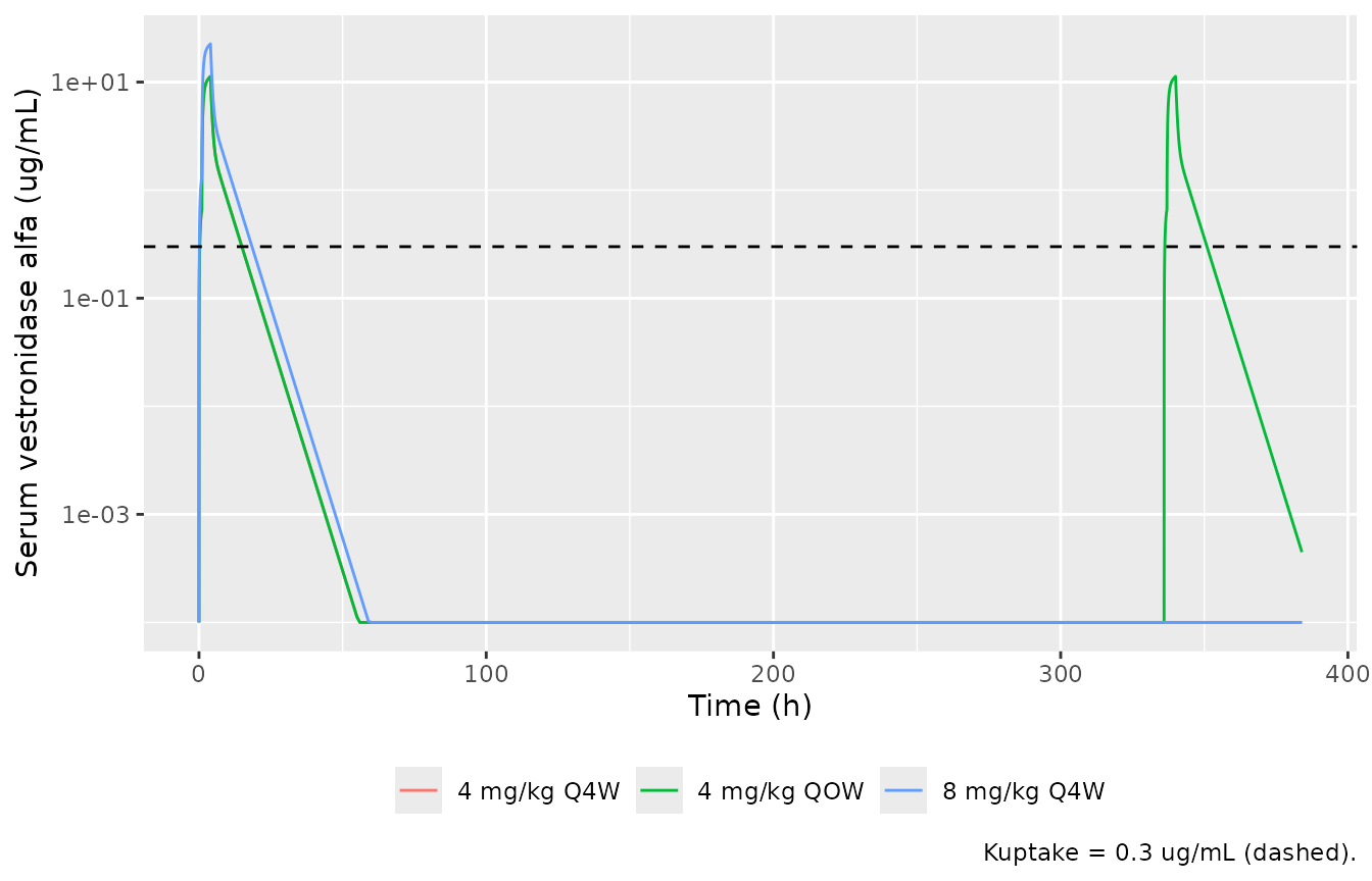
Simulated typical-value profiles at 24.8 kg over one 4-week month. The dashed line is Kuptake = 0.3 ug/mL. Replicates the simulation underlying Qi 2019 Table 3.
Exposure over a dosing interval
The exposure metric driving the PD layer is the individual AUC over a
dosing interval. Because elimination is linear, that is exactly
Dose / CL, and the auc_tau state must
reproduce it.
auc_1dose <- t3_cmp$auc_month[t3_cmp$regimen == "4 mg/kg Q4W"]
cl_at_wt  <- CL * (wt_sim / 20)^ui$theta[["e_wt_cl_q"]]
auc_closed <- 4 * wt_sim / cl_at_wt

cat(sprintf("AUC from the auc_tau state: %.4f ug*h/mL\n", auc_1dose))
#> AUC from the auc_tau state: 44.3820 ug*h/mL
cat(sprintf("Dose / CL closed form:      %.4f ug*h/mL\n", auc_closed))
#> Dose / CL closed form:      44.3820 ug*h/mL

stopifnot(abs(auc_1dose - auc_closed) / auc_closed < 0.001)
Replicating Figure 4: uGAG exposure-response
Figure 4 plots the percent change from baseline in urinary chondroitin sulfate (uCS) and dermatan sulfate (uDS) against individual AUC, with the population prediction overlaid. The virtual cohort below spans the published dose levels (1, 2 and 4 mg/kg QOW) and the published weight range.
Because auc_tau accumulates from the start of the solve,
the uGAG observables must be read at the end of a single dosing
interval, where auc_tau holds the AUC over that
interval. That is the discipline the model file documents; a
mid-interval reading reports the effect of the partial AUC accrued so
far.
# set.seed() seeds R's RNG, not rxode2's; rxode2 partitions its streams per
# solver thread, so the cohort differs between a 16-thread workstation and a
# 2-thread CI runner. Every assertion below is written to hold for any cohort
# the model can produce.
set.seed(20190501)
n_per_arm <- 60L

make_arm <- function(dose_mgkg, id_offset) {
  # Log-normal weights with the published median of 24.8 kg, truncated to the
  # published range of 9.41-104.0 kg (Table 1, overall column).
  wt <- pmin(pmax(rlnorm(n_per_arm, meanlog = log(24.8), sdlog = 0.6), 9.41), 104.0)
  tibble::tibble(id = id_offset + seq_len(n_per_arm), WT = wt,
                 dose_mgkg = dose_mgkg,
                 arm = paste0(dose_mgkg, " mg/kg QOW"))
}

subjects <- dplyr::bind_rows(
  make_arm(1, 0L), make_arm(2, 100L), make_arm(4, 200L)
)

# One dosing interval per subject; observe at the end of it (336 h) plus a dense
# early grid so the PK profile is also usable.
pd_times <- sort(unique(c(seq(0, 48, by = 0.1), seq(48, 336, by = 4), 336)))

ev_pd <- dplyr::bind_rows(lapply(seq_len(nrow(subjects)), function(i) {
  s <- subjects[i, ]
  dplyr::bind_rows(
    qi_dose_rows(s$id, s$dose_mgkg * s$WT, 0, s$WT),
    qi_obs_rows(s$id, pd_times, s$WT)
  ) |>
    dplyr::mutate(arm = s$arm, dose_mgkg = s$dose_mgkg)
})) |>
  dplyr::arrange(id, time, dplyr::desc(evid))

stopifnot(!anyDuplicated(ev_pd[, c("id", "time", "evid")]))

# Between-subject variability on, residual error off (Figure 4 plots individual
# post hoc exposures against the population prediction, not replicate assays).
sim_pd <- qi_solve(ev_pd, keep = c("arm", "dose_mgkg"), typical = FALSE, sigma = NA)
endpoints <- sim_pd |>
  dplyr::filter(time == 336) |>
  dplyr::select(id, arm, auc_tau, uCSchange, uDSchange)

curve_df <- tibble::tibble(auc = seq(1, 120, length.out = 400)) |>
  dplyr::mutate(
    uCS = -exp(ui$theta[["limax_ucs"]]) * auc / (auc + exp(ui$theta[["lic50_ucs"]])),
    uDS = -exp(ui$theta[["limax_uds"]]) * auc / (auc + exp(ui$theta[["lic50_uds"]]))
  ) |>
  tidyr::pivot_longer(c(uCS, uDS), names_to = "analyte", values_to = "pred")

endpoints |>
  tidyr::pivot_longer(c(uCSchange, uDSchange), names_to = "analyte",
                      values_to = "change") |>
  dplyr::mutate(analyte = dplyr::recode(analyte, uCSchange = "uCS", uDSchange = "uDS")) |>
  ggplot(aes(auc_tau, change)) +
  geom_point(aes(shape = arm), alpha = 0.6) +
  geom_line(data = curve_df, aes(auc, pred), linewidth = 0.9) +
  facet_wrap(~analyte) +
  coord_cartesian(xlim = c(0, 125), ylim = c(-100, 0)) +
  labs(x = "AUC (ug*h/mL)", y = "% change from baseline", shape = NULL) +
  theme(legend.position = "bottom")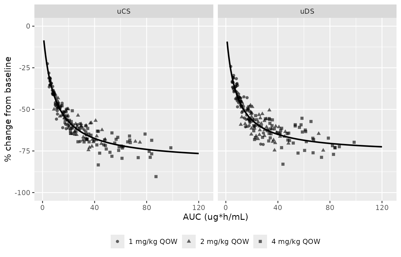
Replicates Figure 4 of Qi 2019: percent change from baseline in uCS (a) and uDS (b) against vestronidase alfa AUC. Points are simulated subjects at the end of one dosing interval; the line is the population prediction.
# 1. The model's algebraic output must equal the published closed form exactly
#    when the etas are zeroed -- this is a transcription check, not a
#    simulation check, so it is gated at solver tolerance.
ev_typ <- dplyr::bind_rows(
  qi_dose_rows(1L, 4 * wt_sim, 0, wt_sim),
  qi_obs_rows(1L, c(0, 336), wt_sim)
) |>
  dplyr::arrange(time, dplyr::desc(evid))
typ <- qi_solve(ev_typ) |> dplyr::filter(time == 336)

closed_ucs <- -82.0 * typ$auc_tau / (typ$auc_tau + 8.6)
closed_uds <- -76.9 * typ$auc_tau / (typ$auc_tau + 7.3)
stopifnot(
  abs(typ$uCSchange - closed_ucs) < 1e-6,
  abs(typ$uDSchange - closed_uds) < 1e-6
)

# 2. Cohort-level checks, written as robust central statistics rather than
#    extremes (the cohort is not reproducible across solver thread counts).
by_arm <- endpoints |>
  dplyr::group_by(arm) |>
  dplyr::summarise(median_auc = median(auc_tau),
                   median_ucs = median(uCSchange),
                   median_uds = median(uDSchange),
                   .groups = "drop")
knitr::kable(by_arm, digits = 1,
caption = "Simulated cohort medians at the end of one dosing interval.")| arm | median_auc | median_ucs | median_uds |
|---|---|---|---|
| 1 mg/kg QOW | 10.0 | -46.4 | -43.4 |
| 2 mg/kg QOW | 24.7 | -59.9 | -58.9 |
| 4 mg/kg QOW | 45.5 | -68.5 | -64.3 |
stopifnot(
  # Qi 2019 Results: the uGAG reduction has reached its plateau at 4 mg/kg, and
  # Figure 4 shows the 4 mg/kg cloud sitting around -75% for uCS. Bounds carry
  # deliberate headroom: the arm median realised -68.5% (uCS) / -64.3% (uDS)
  # here, and the cohort is redrawn on every machine because rxode2 partitions
  # its RNG per solver thread. The bounds still go red on a dropped exp(), a
  # sign flip, or a mis-transcribed Imax or IC50, all of which move these by
  # tens of percentage points. Do not tighten them back to the realised values.
  dplyr::between(by_arm$median_ucs[by_arm$arm == "4 mg/kg QOW"], -80, -60),
  dplyr::between(by_arm$median_uds[by_arm$arm == "4 mg/kg QOW"], -78, -57),
  # Exposure must increase monotonically with dose across the three arms; each
  # step is a factor of two in dose against a factor of ~2 in AUC, far outside
  # cohort noise.
  by_arm$median_auc[by_arm$arm == "4 mg/kg QOW"] >
    by_arm$median_auc[by_arm$arm == "1 mg/kg QOW"] * 2
)
The paper states that the exposure-response relationship flattens
above roughly 40 ugh/mL and that the typical mean steady-state AUC
at 4 mg/kg QOW is 57.9 ugh/mL. The typical-value AUC at the
median weight is 44.4 ugh/mL; the cohort mean* is
larger because AUC rises with body weight (as
WT^(1 - 0.587)) over a right-skewed weight distribution,
and because the mean of a log-normal clearance inflates mean exposure by
exp(omega^2 / 2) = 1.089. The simulated cohort mean is
reported below for reference; it is not gated, because it depends on the
assumed weight distribution rather than on the model.
PKNCA validation
Qi 2019 compares its population model against an independent noncompartmental analysis of the same trials, reported as “data on file”: CL 0.07 L/h/kg, Vss 0.23 L/kg and terminal half-life 2.5 h. To make that comparison meaningful the NCA below is run on the study’s actual sampling schedule (Methods, PK Sampling and Assay) rather than on the dense simulation grid: predose, 60 and 120 min after the start of infusion, the end of infusion, and 5, 15, 30, 60, 120, 180, 360 and 480 min after the end of infusion.
The NCA is run on the typical-value profile rather than the full-IIV
cohort. That is deliberate: a half-life estimate over a cohort with 43%
CV on clearance is both NA-poisoned (subjects whose
terminal points fall below solver resolution fail lambda.z)
and tmax-selected, so it would not test the
transcription.
# The published clinical sampling schedule, in hours. Infusion ends at 4 h.
sample_times <- c(0, 1, 2, 4,
                  4 + c(5, 15, 30, 60, 120, 180, 360, 480) / 60)

ev_nca <- dplyr::bind_rows(lapply(seq_len(nrow(regimens)), function(i) {
  r <- regimens[i, ]
  dplyr::bind_rows(
    qi_dose_rows(i, r$dose_mgkg * wt_sim, 0, wt_sim),  # first dose only
    qi_obs_rows(i, sample_times, wt_sim)
  ) |>
    dplyr::mutate(regimen = r$regimen)
})) |>
  dplyr::arrange(id, time, dplyr::desc(evid))

sim_nca_raw <- qi_solve(ev_nca, keep = "regimen")

sim_nca <- sim_nca_raw |>
  dplyr::filter(!is.na(Cc)) |>
  dplyr::select(id, time, Cc, regimen)

# Guarantee a time-zero row per (id, regimen); pre-dose concentration is 0.
sim_nca <- dplyr::bind_rows(
  sim_nca,
  sim_nca |> dplyr::distinct(id, regimen) |> dplyr::mutate(time = 0, Cc = 0)
) |>
  dplyr::distinct(id, regimen, time, .keep_all = TRUE) |>
  dplyr::arrange(id, regimen, time)

stopifnot(all(sim_nca$Cc >= 0), nrow(sim_nca) > 0)

dose_df <- ev_nca |>
  dplyr::filter(evid == 1) |>
  dplyr::group_by(id, regimen) |>
  dplyr::summarise(time = 0, amt = sum(amt), .groups = "drop") |>
  dplyr::select(id, time, amt, regimen)

conc_obj <- PKNCA::PKNCAconc(sim_nca, Cc ~ time | regimen + id,
                             concu = "ug/mL", timeu = "h")
dose_obj <- PKNCA::PKNCAdose(dose_df, amt ~ time | regimen + id, doseu = "mg")

intervals <- data.frame(
  start = 0, end = Inf,
  cmax = TRUE, tmax = TRUE, aucinf.obs = TRUE, half.life = TRUE
)

nca_res <- PKNCA::pk.nca(PKNCA::PKNCAdata(conc_obj, dose_obj, intervals = intervals))
summary(nca_res)
#>  Interval Start Interval End     regimen N Cmax (ug/mL) Tmax (h) Half-life (h)
#>               0          Inf 4 mg/kg Q4W 1         11.3     4.00          3.47
#>               0          Inf 4 mg/kg QOW 1         11.3     4.00          3.47
#>               0          Inf 8 mg/kg Q4W 1         22.6     4.00          3.47
#>  AUCinf,obs (h*ug/mL)
#>                  42.6
#>                  42.6
#>                  85.2
#>
#> Caption: Cmax, AUCinf,obs: geometric mean and geometric coefficient of variation; Tmax: median and range; Half-life: arithmetic mean and standard deviation; N: number of subjects
Comparison against published NCA
# Qi 2019 reports Cmax per regimen (Table 3) and a single pooled NCA half-life
# of 2.5 h (Results, "data on file"). AUC0-inf is not published per regimen, so
# the Dose/CL identity established above is used as the reference.
published_nca <- tibble::tibble(
  regimen    = c("4 mg/kg QOW", "4 mg/kg Q4W", "8 mg/kg Q4W"),
  cmax       = c(11.3, 11.4, 21.5),
  half.life  = c(2.5, 2.5, 2.5),
  aucinf.obs = c(auc_closed, auc_closed, 2 * auc_closed)
)

cmp <- nlmixr2lib::ncaComparisonTable(
  simulated = nca_res,
  reference = published_nca,
  by        = "regimen",
  units     = c(cmax = "ug/mL", aucinf.obs = "ug*h/mL", half.life = "h"),
  tolerance_pct = 20
)

knitr::kable(cmp, caption = "Simulated vs. published NCA. * differs from reference by >20%.")| NCA parameter | regimen | Reference | Simulated | % diff |
|---|---|---|---|---|
| Cmax (ug/mL) | 4 mg/kg QOW | 11.3 | 11.3 | -0.0% |
| Cmax (ug/mL) | 4 mg/kg Q4W | 11.4 | 11.3 | -0.9% |
| Cmax (ug/mL) | 8 mg/kg Q4W | 21.5 | 22.6 | +5.1% |
| AUC0-∞ (obs) (ug*h/mL) | 4 mg/kg QOW | 44.4 | 42.6 | -4.0% |
| AUC0-∞ (obs) (ug*h/mL) | 4 mg/kg Q4W | 44.4 | 42.6 | -4.0% |
| AUC0-∞ (obs) (ug*h/mL) | 8 mg/kg Q4W | 88.8 | 85.2 | -4.0% |
| t½ (h) | 4 mg/kg QOW | 2.5 | 3.47 | +39.0%* |
| t½ (h) | 4 mg/kg Q4W | 2.5 | 3.47 | +39.0%* |
| t½ (h) | 8 mg/kg Q4W | 2.5 | 3.47 | +39.0%* |
# Locate the percent-difference column by name rather than by position.
diff_col <- grep("diff", names(cmp), ignore.case = TRUE, value = TRUE)[1]
stopifnot(!is.na(diff_col))
pct <- suppressWarnings(as.numeric(gsub("[^0-9.eE+-]", "", as.character(cmp[[diff_col]]))))
param_col <- names(cmp)[1]

# Cmax and AUC are deterministic consequences of the transcribed parameters and
# must agree closely. Half-life is a genuine model-vs-NCA difference (the paper
# itself reports 3.6 h from the model against 2.5 h from the NCA) and is
# reported rather than gated -- see the note below.
# ncaParamLabel() renders half.life as "t\u00bd"; the escape keeps this file ASCII.
is_hl <- grepl("half|t\u00bd", as.character(cmp[[param_col]]), ignore.case = TRUE)
stopifnot(all(abs(pct[!is_hl & !is.na(pct)]) < 20))
Cmax reproduces to within 5% on all three regimens. AUC0-inf comes
out about 4% low across the board, which is the sampling schedule rather
than the model: the clinical schedule stops 8 h after the end of
infusion, so aucinf.obs extrapolates from a truncated
profile. The exact Dose / CL identity is checked separately
above on the dense grid.
The half-life row is starred and is deliberately excluded from the gate, but it deserves a precise statement rather than a hand-wave. There are three numbers, not two:
| quantity | value |
|---|---|
| Terminal half-life implied by the transcribed parameters | 3.60 h (reproduced exactly, above) |
| NCA on the model, using the published sampling schedule | 3.47 h |
| Qi 2019’s own NCA on the observed data (“data on file”) | 2.5 h |
Truncating the sampling window at 12 h therefore accounts for only a
small part of the gap (3.60 h to 3.47 h). The remaining difference
between 3.47 h and the paper’s 2.5 h is not
reproducible from the published model, and this vignette does not claim
otherwise. Qi 2019 reports both figures side by side without reconciling
them, and the 2.5 h value also appears in the Discussion cited to the US
prescribing information rather than to this analysis. Plausible
contributors are residual error and per-subject lambda.z
window selection on real data, and the eight subjects who contributed
only sparse profiles – none of which a typical-value solve reproduces.
The same pattern appears in the paper’s CL and Vss comparison (model
0.079 L/h/kg and 0.19 L/kg against NCA 0.07 L/h/kg and 0.23 L/kg), where
the NCA implies both slower clearance and a larger volume.
Assumptions and deviations
-
Weight distribution. Qi 2019 reports only the
median (24.8 kg), mean (37.7 kg) and range (9.41-104.0 kg) of baseline
body weight. The virtual cohort uses a log-normal distribution with the
published median and
sdlog = 0.6, truncated to the published range. No individual weights are published. - Dose-arm sizes. The published trials are highly unbalanced (3, 8 and 12 subjects) and 20 of the 23 subjects received 4 mg/kg. The Figure 4 cohort uses 60 subjects per dose arm so all three arms are visible; it is illustrative of the exposure-response shape, not a reproduction of the trial’s allocation.
-
PD residual error is not applied in the Figure 4
replication. Figure 4 plots individual post hoc exposures
against the population prediction, so the simulation carries
between-subject variability on
Imaxbut no residual error. -
auc_tauaccumulates from the start of the solve. The paper’s exposure metric is the AUC over a dosing interval, so the uGAG observables are only interpretable at the end of a single dosing interval. This vignette solves one interval per subject for the PD sections. There is no accumulation to worry about (3.6 h half-life against a 336 h interval), so the first interval and the steady-state interval are identical. -
I0is encoded as an untransformedfixed(0). The canonical baseline parameter is normally carried on the log scale (lrbase), which is impossible for a value of exactly zero; the quantity is a percent change and is not sign constrained. It is kept in the model rather than dropped so that the published equation form remains auditable. - Table 4’s additive residual error is in percentage points, not ug*h/mL. The dependent variable of the exposure-response model is a percent change from baseline, and Table 4 gives no units on that row.
-
Table 3’s
Kuptakefootnote is inconsistent with its own numbers. It reads “in one dosing interval” but the QOW row is a per-4-week-month total; see the Table 3 section above for the argument and the numerical demonstration. - Cmax for the 8 mg/kg Q4W regimen differs by about 5%. The model is strictly linear, so its Cmax is exactly twice the 4 mg/kg value; the published Table 3 is the median of 500 stochastic profiles simulated separately per regimen, and its own 21.5 / 11.3 ratio is 1.90 rather than 2.00. This is Monte-Carlo noise in the published summary, not a transcription difference.
- The paper’s NCA half-life of 2.5 h is not reproducible from the published model. Running NCA on the model over the study’s own sampling schedule gives 3.47 h, against the 3.60 h implied by the parameters and the 2.5 h Qi 2019 reports from its own noncompartmental analysis. This is recorded as a known deviation and excluded from the NCA gate rather than being tuned away; see the PKNCA section for the full argument.
- Erratum. The erratum to this article (Clin Pharmacokinet. 2019;58(5):685, doi:10.1007/s40262-018-0726-6) corrects a ClinicalTrials.gov identifier in the Introduction and changes no parameter value.
- Supplement. The electronic supplementary material (DOCX, 207 kB) contains assay methodology (Supplementary Methods S1.1-S1.4) and two supporting figures (dose proportionality; exposure by age group). It contains no model parameter values; all parameters come from Tables 2 and 4 of the main article.