PEGasparaginase (Kloos 2021)
Source:vignettes/articles/Kloos_2021_pegasparaginase.Rmd
Kloos_2021_pegasparaginase.Rmd
library(nlmixr2lib)
library(rxode2)
#> rxode2 5.1.8 using 2 threads (see ?getRxThreads)
#>   no cache: create with `rxCreateCache()`
library(dplyr)
#>
#> Attaching package: 'dplyr'
#> The following objects are masked from 'package:stats':
#>
#>     filter, lag
#> The following objects are masked from 'package:base':
#>
#>     intersect, setdiff, setequal, union
library(tidyr)
library(ggplot2)
library(PKNCA)
#>
#> Attaching package: 'PKNCA'
#> The following object is masked from 'package:stats':
#>
#>     filter
PEGasparaginase population PK in pediatric ALL
Simulate intravenous PEGasparaginase (pegaspargase; Oncaspar) asparaginase activity-time profiles in pediatric acute lymphoblastic leukemia (ALL) patients using the final population PK model of Kloos et al. (2021).
The structural model is a one-compartment linear disposition with IV input (a 1 h infusion into the central compartment) and a split-point time-dependent clearance: clearance is constant for the first 12.7 days after a dose and then rises linearly with time after dose, as the polyethylene glycol moiety is hydrolyzed from the molecule and the residual native E. coli asparaginase is cleared much faster. Both clearance and volume of distribution are normalized to body surface area (a linear proportionality, not an allometric power). Clearance is 38% higher during an active infection and 11-19% lower outside induction.
- Article: https://doi.org/10.3324/haematol.2019.242289
- Erratum (corrected Table 5): https://doi.org/10.3324/haematol.2023.283685
- PubMed: https://pubmed.ncbi.nlm.nih.gov/32327497/
Population
The model was developed on 92 index-dataset patients (816 asparaginase activity samples) with newly diagnosed ALL treated per the Dutch Childhood Oncology Group (DCOG) ALL-11 protocol at Sophia Children’s Hospital - Erasmus MC between November 2014 and May 2017, supplemented with trough samples from the Dutch national therapeutic-drug-monitoring program. From Kloos 2021 Supplemental Table 2 and Table 1:
- Age median 4.8 years (IQR 3.3-8.2); protocol eligibility 1-18 years
- Weight median 19.2 kg (IQR 14.9-29.3)
- BSA median 0.76 m^2 (IQR 0.65-1.05)
- Sex: 51 male (55%) / 41 female (45%)
- Risk group: standard 13 (14%), medium 76 (83%), high 2 (2%), not stratified 1 (1%)
- 19 patients had at least one infection episode
A further 28 patients / 405 samples, obtained by randomly selecting
25% of the total 120-patient population, formed an independent
external-validation dataset. Race / ethnicity is not reported. The same
metadata is available programmatically via
readModelDb("Kloos_2021_pegasparaginase")$population.
All patients received three fixed 1,500 IU/m^2 PEGasparaginase doses biweekly during induction (protocols 1A and 1B, at days 12, 26 and 40 of the protocol); subsequent doses were individualized by therapeutic drug monitoring. Each dose was infused intravenously over 1 hour. Asparaginase activity was measured by the L-aspartic beta-hydroxamate (AHA) assay (LLQ 10 IU/L); values below the LLQ were excluded from the analysis.
Source trace
The per-parameter origin is recorded as an in-file comment next to
each ini() entry in
inst/modeldb/specificDrugs/Kloos_2021_pegasparaginase.R.
The table below collects the mapping in one place for reviewer
audit.
| Element | Source location | Value / form |
|---|---|---|
| One-compartment IV model | Kloos 2021 Results, Structural model; Supplement, Supplemental Results |
d/dt(central) = -kel * central; adding a second
compartment did not improve the fit |
| CL typical (per m^2) | Kloos 2021 Table 2, Final model | 0.084 L/day/m^2 (RSE 4.4%; bootstrap 0.084, 95% CI 0.078-0.090) |
| Vd typical (per m^2) | Kloos 2021 Table 2, Final model | 0.94 L/m^2 (RSE 4.5%; bootstrap 0.94, 95% CI 0.87-1.01) |
| Time-dependent CL slope | Kloos 2021 Table 2, Final model (“Slope CL_ind”) | 0.082 L/day/m^2/day (RSE 20.5%; bootstrap 0.080, 95% CI 0.052-0.115) |
| Split point | Kloos 2021 Table 2, Final model | 12.7 days (RSE 0.2%; bootstrap 12.7, 95% CI 11.8-13.1) |
| BSA scaling of CL and Vd | Kloos 2021 Table 2 equations; Supplement, Supplemental Results |
CL = Theta1 * ... * BSA;
Vd = Theta3 * e^(Theta4 * eta) * BSA (linear, no
exponent) |
| Infection effect on CL | Kloos 2021 Table 2, Final model |
1.38^DIS_INFECT_ACTIVE (RSE 10.5%; bootstrap 95% CI
1.15-1.67) |
| Treatment phase 1A | Kloos 2021 Table 2, Final model | Reference (all TRTPH_ indicators 0) |
| Treatment phase 1B | Kloos 2021 Table 2, Final model |
1 (fix) – pooled with 1A; only two high-risk patients,
not estimable |
| Treatment phase M | Kloos 2021 Table 2, Final model |
0.87^TRTPH_M (RSE 5.2%; bootstrap 95% CI
0.80-0.95) |
| Treatment phase MR intensification | Kloos 2021 Table 2, Final model |
0.89^TRTPH_MR_INTENS (RSE 5.2%; bootstrap 95% CI
0.82-0.98) |
| Treatment phase MR maintenance | Kloos 2021 Table 2, Final model |
0.81^TRTPH_MR_MAINT (RSE 3.9%; bootstrap 95% CI
0.75-0.86) |
| Treatment phase SR protocol IV | Kloos 2021 Table 2, Final model |
0.81^TRTPH_SR_IV (RSE 6.5%; bootstrap 95% CI
0.73-0.90) |
| CL-to-Vd shared eta scaling | Kloos 2021 Table 2 (“Fractional increase IIV-Vd”); Supplement equation for Vd | 1.26 (RSE 10.2%; bootstrap 1.28, 95% CI 0.98-1.51) |
| IIV on CL | Kloos 2021 Table 2, Final model | 19.7% CV ->
omega^2 = log(1 + 0.197^2) = 0.038077
|
| IOV on CL | Kloos 2021 Table 2, Final model; Supplement, Supplemental Methods | 23.6% CV -> pi^2 = log(1 + 0.236^2) = 0.054197;
occasion = administration of a new dose |
| Residual error | Kloos 2021 Table 2, Final model; Supplement, Supplemental Results | Combined: proportional 17.0% + additive 20.2 IU/L |
| Published half-lives (structural model) | Kloos 2021 Results, Structural model | 8.5 days for the first 12.9 days; 4.1 days after 1 further day; 2.7 days after 2 |
| Native-asparaginase convergence | Kloos 2021 Discussion | CL rises to a value comparable to native E. coli asparaginase (half-life 1.3 days) “after several days” |
| Starting-dose guideline | Kloos 2021 Table 4 | Protocol 1A, target trough 100 IU/L: loading 800 IU/m^2, maintenance 600 IU/m^2 |
| Dose-adjustment nomogram | Kloos 2021 Table 5, as corrected by the 2023 erratum | See “Errata” below |
Covariate column naming
| Source column | Canonical column used here | Notes |
|---|---|---|
BSA |
BSA (m^2) |
Mosteller formula. Scales CL and Vd linearly (no exponent). |
INFECTION |
DIS_INFECT_ACTIVE (binary, time-varying) |
New canonical registered in
inst/references/covariate-columns.md. Kloos 2021 defines an
infection as fever >38 C plus hospital admission or prescription of
antibiotics. |
Treatment phase 1B
|
TRTPH_1B (binary, time-varying) |
New TRTPH_<phase> canonical family. Effect fixed
to 1 (pooled with the 1A reference). |
Treatment phase M
|
TRTPH_M |
New TRTPH_<phase> canonical family. |
Treatment phase MRG intens.
|
TRTPH_MR_INTENS |
New TRTPH_<phase> canonical family. |
Treatment phase MRG maint.
|
TRTPH_MR_MAINT |
New TRTPH_<phase> canonical family. |
Treatment phase SRG protocol IV
|
TRTPH_SR_IV |
New TRTPH_<phase> canonical family. |
| occasion (= a new dose) |
OCC (integer) |
Existing canonical; decomposed to
oc1/oc2/oc3 inside
model(). |
Protocol 1A (induction) is the reference phase and is encoded as all
TRTPH_ indicators 0.
The additive-slope reading (structural decision)
Kloos 2021 is internally inconsistent about whether the time-dependent clearance slope is additive or multiplicative. This model implements the additive form. Because that choice changes late-time behaviour by a factor of 2-3, the evidence is laid out here before any simulation, and the half-life check below is the validation that discriminates the two readings.
The two readings, with the same reported numbers:
-
Additive –
CL = Theta1 + Theta2 * (TAD - split), withTheta2 = 0.082 L/day/m^2/day -
Multiplicative –
CL = Theta1 * (1 + Theta2 * (TAD - split)), withTheta2now in units of1/day
The printed equations in Table 2 and in the Online Supplementary
Appendix give the multiplicative form. Everything else in the paper
gives the additive form: the Table 2 row label states the parameter’s
units as L/day/m^2/day (absolute clearance per day, which
is meaningless in the multiplicative form), and the abstract, Results
(Structural model) and Results (Covariate analysis) all phrase it as
clearance “increasing by 0.082 L/day/m^2/day thereafter”.
The decisive evidence is that the paper publishes three half-lives for its structural model, which only one reading reproduces.
# Kloos 2021 STRUCTURAL model (Table 2, "Structural model" column):
th1_struct <- 0.075   # L/day/m^2
th2_struct <- 0.079   # L/day/m^2/day
vd_struct  <- 0.92    # L/m^2

days_after_split <- c(0, 1, 2)

halflife_check <- tibble(
  `Days after split point` = days_after_split,
  `Published (Kloos 2021 Results)` = c(8.5, 4.1, 2.7),
  `Additive reading` =
    log(2) * vd_struct / (th1_struct + th2_struct * days_after_split),
  `Multiplicative reading` =
    log(2) * vd_struct / (th1_struct * (1 + th2_struct * days_after_split))
)

knitr::kable(
  halflife_check,
  digits  = 2,
  caption = paste(
    "PEGasparaginase half-life (days) under the two readings of the",
    "time-dependent-clearance slope, versus the values Kloos 2021 publishes",
    "for its own structural model (Results, Structural model)."
  )
)| Days after split point | Published (Kloos 2021 Results) | Additive reading | Multiplicative reading |
|---|---|---|---|
| 0 | 8.5 | 8.50 | 8.50 |
| 1 | 4.1 | 4.14 | 7.88 |
| 2 | 2.7 | 2.74 | 7.34 |
The additive reading reproduces all three published half-lives to two significant figures; the multiplicative reading misses the second and third by factors of 1.9 and 2.7. A second, independent check points the same way: Kloos 2021’s Discussion states that clearance rises to a value comparable to native E. coli asparaginase (half-life 1.3 days) “after several days”.
# Final-model parameters (Table 2, "Final model" column).
th1 <- 0.084; th2 <- 0.082; vd <- 0.94
cl_native <- log(2) * vd / 1.3   # CL giving a 1.3 day half-life

tibble(
  Reading = c("Additive", "Multiplicative"),
  `Days after split point to reach a 1.3 day half-life` = c(
    (cl_native - th1) / th2,
    (cl_native / th1 - 1) / th2
  )
) |>
  knitr::kable(
    digits  = 1,
    caption = paste(
      "Time for clearance to reach native-E. coli-asparaginase level",
      "(half-life 1.3 days). Kloos 2021 Discussion says 'after several days'."
    )
)| Reading | Days after split point to reach a 1.3 day half-life |
|---|---|
| Additive | 5.1 |
| Multiplicative | 60.6 |
The additive reading gives ~5 days (“several days”); the multiplicative reading gives ~61 days, well beyond the 30-day observation window of Kloos 2021 Figure 2. This deviation from the two printed equations is recorded again under “Assumptions and deviations” below.
Virtual cohort
Kloos 2021 does not publish individual baseline covariates. The cohort below reproduces the published BSA distribution (Supplemental Table 2: median 0.76 m^2, IQR 0.65-1.05) with a log-normal whose median and IQR match, and clips to the 0.52-2.3 m^2 range the authors used for their own Monte Carlo simulations (Supplement, Supplemental Results, Simulations).
set.seed(2021)
n_subj <- 200

# The published BSA distribution is right-skewed (median 0.76, IQR 0.65-1.05),
# more so than any log-normal with the same median can reproduce. Sampling
# from a piecewise-linear inverse CDF through the published quantiles, with
# tails running to the 0.52-2.3 m^2 range the authors used for their own Monte
# Carlo simulations, reproduces the published summary by construction.
bsa_p <- c(0,    0.25, 0.50, 0.75, 1.0)
bsa_q <- c(0.52, 0.65, 0.76, 1.05, 2.3)

pop <- tibble(
  id  = seq_len(n_subj),
  BSA = approx(bsa_p, bsa_q, xout = runif(n_subj))$y
)

tibble(
  Source = c("Kloos 2021 Supplemental Table 2", "Virtual cohort"),
  Median = c(0.76, median(pop$BSA)),
  `Q1`   = c(0.65, quantile(pop$BSA, 0.25)),
  `Q3`   = c(1.05, quantile(pop$BSA, 0.75))
) |>
knitr::kable(digits = 2, caption = "Body surface area (m^2): published versus virtual cohort.")| Source | Median | Q1 | Q3 |
|---|---|---|---|
| Kloos 2021 Supplemental Table 2 | 0.76 | 0.65 | 1.05 |
| Virtual cohort | 0.75 | 0.64 | 1.01 |
Event table
Doses are given in IU (1,500 IU/m^2 multiplied by each subject’s BSA)
and infused over 1 hour. The model’s time unit is days,
so the infusion duration is 1/24 day. Observation rows are
placed on the central compartment, the ODE state;
Cc (the asparaginase activity level) is returned as a
column at those rows.
mod <- readModelDb("Kloos_2021_pegasparaginase")

# Build the random-effect covariance explicitly. rxSolve() reuses the omega of
# a previous solve in the same session unless one is supplied, which silently
# either strips IIV from a population run or injects it into a typical-value
# run. Values are the Kloos 2021 Table 2 final-model variances (see the model
# file): IIV CL 19.7% CV and IOV CL 23.6% CV, each as log(1 + CV^2).
eta_names <- c("etalcl", "etaiov_cl_1", "etaiov_cl_2", "etaiov_cl_3")
om <- diag(c(log(1 + 0.197^2), rep(log(1 + 0.236^2), 3)))
dimnames(om) <- list(eta_names, eta_names)

infusion_dur_d <- 1 / 24
dose_iu_per_m2 <- 1500

# Observation grid: dense early, then daily out to 30 days (matching the
# x-axis of Kloos 2021 Figure 2). A time-zero record is included so PKNCA
# does not extrapolate an AUC start before the first measurement.
obs_times <- sort(unique(c(
  0,
  seq(0,  1, by = 1 / 24),   # infusion and immediate post-infusion
  seq(1, 13, by = 0.25),     # constant-clearance window
  seq(13, 30, by = 0.1)      # induced-clearance window (rapid decline)
)))

# Protocol 1A induction, no infection: the model's reference condition.
covs_1a <- function(d) {
  d |>
    mutate(
      DIS_INFECT_ACTIVE = 0L,
      TRTPH_1B          = 0L,
      TRTPH_M           = 0L,
      TRTPH_MR_INTENS   = 0L,
      TRTPH_MR_MAINT    = 0L,
      TRTPH_SR_IV       = 0L,
      OCC               = 1L
    )
}

doses <- pop |>
  mutate(
    time = 0,
    amt  = dose_iu_per_m2 * BSA,      # IU
    dur  = infusion_dur_d,            # 1 h expressed in days
    evid = 1L,
    cmt  = "central"
  ) |>
  covs_1a() |>
  select(id, time, amt, dur, evid, cmt, BSA,
         DIS_INFECT_ACTIVE, starts_with("TRTPH_"), OCC)

obs <- tidyr::crossing(pop |> select(id, BSA), time = obs_times) |>
  mutate(
    amt  = NA_real_,
    dur  = NA_real_,
    evid = 0L,
    cmt  = "central"
  ) |>
  covs_1a() |>
  select(id, time, amt, dur, evid, cmt, BSA,
         DIS_INFECT_ACTIVE, starts_with("TRTPH_"), OCC)

events <- bind_rows(doses, obs) |>
  arrange(id, time, desc(evid)) |>
  as.data.frame()
# Pass omega explicitly: rxSolve() will otherwise reuse the omega of a
# previous solve in the same session.
sim <- rxode2::rxSolve(
  mod, events,
  omega      = om,
  keep       = c("BSA", "DIS_INFECT_ACTIVE", "OCC"),
  returnType = "data.frame"
)
#> ℹ parameter labels from comments will be replaced by 'label()'
#> Warning: some etas defaulted to non-mu referenced, possible parsing error: etaiov_cl_1, etaiov_cl_2, etaiov_cl_3
#> as a work-around try putting the mu-referenced expression on a simple line

# rxSolve occasionally returns fewer subjects than requested; assert.
stopifnot(
  dplyr::n_distinct(sim$id) == n_subj,
  !anyNA(sim$Cc)
)
Replicating Kloos 2021 Figure 2
Figure 2 of Kloos 2021 plots asparaginase activity against time after administration on a log scale, and its caption draws attention to the fact that “the asparaginase activity levels nonlinearly decline after 12.7 days”. The split-point clearance model reproduces exactly that break.
sim_summary <- sim |>
  filter(time > 0, Cc > 0) |>
  group_by(time) |>
  summarise(
    median = median(Cc),
    q05    = quantile(Cc, 0.05),
    q95    = quantile(Cc, 0.95),
    .groups = "drop"
  )

ggplot(sim_summary, aes(x = time)) +
  geom_ribbon(aes(ymin = q05, ymax = q95), alpha = 0.20, fill = "steelblue") +
  geom_line(aes(y = median), color = "steelblue", linewidth = 0.9) +
  geom_vline(xintercept = 12.7, linetype = "dotted") +
  geom_hline(yintercept = 100, linetype = "dashed", color = "firebrick") +
  annotate("text", x = 12.9, y = 2000, hjust = 0, size = 3,
           label = "split point 12.7 d") +
  annotate("text", x = 0.5, y = 130, hjust = 0, size = 3, color = "firebrick",
           label = "target 100 IU/L") +
  scale_y_log10(labels = scales::label_comma()) +
  coord_cartesian(xlim = c(0, 30), ylim = c(1, 3000)) +
  labs(
    x        = "Time after administration (days)",
    y        = "Asparaginase activity level (IU/L)",
    title    = "Simulated single-dose PEGasparaginase activity",
    subtitle = sprintf("1,500 IU/m^2 IV over 1 h, N = %d virtual patients, protocol 1A", n_subj),
    caption  = "Replicates Kloos 2021 Figure 2: nonlinear decline beginning at the 12.7 day split point."
  ) +
  theme_bw()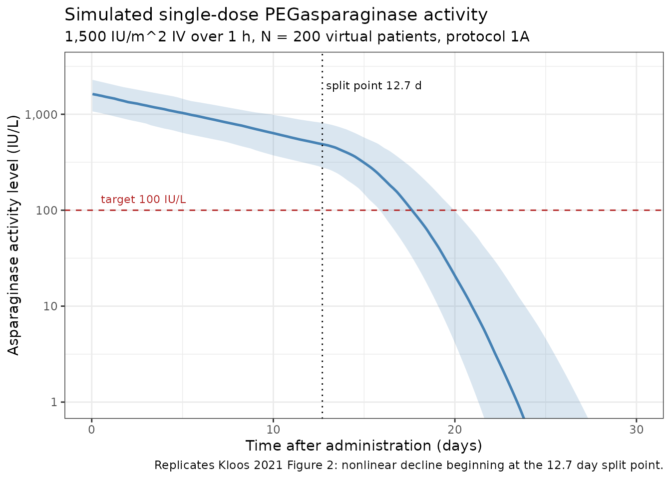
Instantaneous half-life across the dosing interval
The shipped final model’s own instantaneous half-life,
ln(2) * Vd / CL(t), is recovered directly from the solved
cl and vc columns. It is flat at 7.8 days
until the split point and then collapses.
# Use a typical-value solve (random effects zeroed) rather than the median of
# the population run: the half-life is a typical-value property, and a median
# over 200 subjects carries a couple of percent of Monte Carlo noise that would
# obscure the comparison against the closed form.
hl <- rxode2::rxSolve(
  rxode2::zeroRe(mod),
  filter(events, id == 1) |> mutate(BSA = median(pop$BSA)),
  omega = NA, returnType = "data.frame"
) |>
  mutate(thalf = log(2) * vc / cl) |>
  select(time, thalf)
#> ℹ parameter labels from comments will be replaced by 'label()'
#> Warning: some etas defaulted to non-mu referenced, possible parsing error: etaiov_cl_1, etaiov_cl_2, etaiov_cl_3
#> as a work-around try putting the mu-referenced expression on a simple line
#> Warning: some etas defaulted to non-mu referenced, possible parsing error: etaiov_cl_1, etaiov_cl_2, etaiov_cl_3
#> as a work-around try putting the mu-referenced expression on a simple line

ggplot(hl, aes(time, thalf)) +
  geom_line(color = "darkorange3", linewidth = 0.9) +
  geom_vline(xintercept = 12.7, linetype = "dotted") +
  geom_hline(yintercept = 1.3, linetype = "dashed", color = "grey40") +
  annotate("text", x = 20, y = 1.9, size = 3, color = "grey30",
           label = "native E. coli asparaginase (1.3 d)") +
  labs(
    x = "Time after administration (days)",
    y = "Instantaneous half-life (days)",
    title = "Time-dependent clearance shortens the PEGasparaginase half-life",
    caption = "Kloos 2021 Discussion: clearance approaches native asparaginase levels after several days."
  ) +
  theme_bw()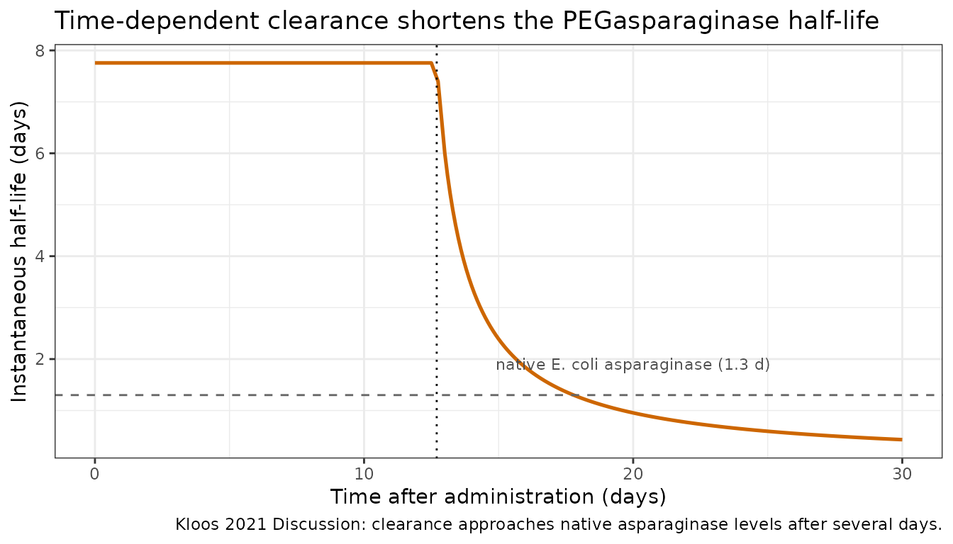
pick <- function(tt) hl$thalf[which.min(abs(hl$time - tt))]

tibble(
  `Time after dose (days)` = c(5, 12.5, 13.7, 14.7, 17.7),
  `Typical-value simulated half-life (days)` = vapply(
    c(5, 12.5, 13.7, 14.7, 17.7), pick, numeric(1)
  ),
  `Analytic ln(2) * Vd / CL (days)` = log(2) * 0.94 /
    (0.084 + 0.082 * pmax(0, c(5, 12.5, 13.7, 14.7, 17.7) - 12.7))
) |>
  knitr::kable(
    digits  = 2,
    caption = paste(
      "Final-model instantaneous half-life: typical-value simulation versus",
      "the closed-form value. Agreement confirms the model encodes the",
      "additive slope as intended."
    )
)| Time after dose (days) | Typical-value simulated half-life (days) | Analytic ln(2) * Vd / CL (days) |
|---|---|---|
| 5.0 | 7.76 | 7.76 |
| 12.5 | 7.76 | 7.76 |
| 13.7 | 3.93 | 3.93 |
| 14.7 | 2.63 | 2.63 |
| 17.7 | 1.32 | 1.32 |
Covariate effects on clearance
Typical-value profiles under each treatment phase and with / without an active infection, for a patient with the cohort-median BSA. Random effects are zeroed so the curves are the model’s typical values.
mod_tv <- rxode2::zeroRe(mod)
#> ℹ parameter labels from comments will be replaced by 'label()'
#> Warning: some etas defaulted to non-mu referenced, possible parsing error: etaiov_cl_1, etaiov_cl_2, etaiov_cl_3
#> as a work-around try putting the mu-referenced expression on a simple line
#> Warning: some etas defaulted to non-mu referenced, possible parsing error: etaiov_cl_1, etaiov_cl_2, etaiov_cl_3
#> as a work-around try putting the mu-referenced expression on a simple line

scenario_covs <- tribble(
  ~scenario,                      ~DIS_INFECT_ACTIVE, ~TRTPH_1B, ~TRTPH_M, ~TRTPH_MR_INTENS, ~TRTPH_MR_MAINT, ~TRTPH_SR_IV,
  "Protocol 1A (reference)",                      0L,        0L,       0L,               0L,              0L,           0L,
  "Protocol 1A + infection",                      1L,        0L,       0L,               0L,              0L,           0L,
  "Protocol M",                                   0L,        0L,       1L,               0L,              0L,           0L,
  "MR intensification",                           0L,        0L,       0L,               1L,              0L,           0L,
  "MR maintenance",                               0L,        0L,       0L,               0L,              1L,           0L,
  "SR protocol IV",                               0L,        0L,       0L,               0L,              0L,           1L
)

bsa_med <- median(pop$BSA)

tv_events <- scenario_covs |>
  mutate(id = row_number()) |>
  rowwise() |>
  do({
    row <- .
    d <- tibble(time = 0, amt = dose_iu_per_m2 * bsa_med,
                dur = infusion_dur_d, evid = 1L, cmt = "central")
    o <- tibble(time = obs_times, amt = NA_real_, dur = NA_real_,
                evid = 0L, cmt = "central")
    bind_rows(d, o) |>
      mutate(id = row$id, scenario = row$scenario, BSA = bsa_med,
             DIS_INFECT_ACTIVE = row$DIS_INFECT_ACTIVE,
             TRTPH_1B = row$TRTPH_1B, TRTPH_M = row$TRTPH_M,
             TRTPH_MR_INTENS = row$TRTPH_MR_INTENS,
             TRTPH_MR_MAINT = row$TRTPH_MR_MAINT,
             TRTPH_SR_IV = row$TRTPH_SR_IV, OCC = 1L)
  }) |>
  ungroup() |>
  arrange(id, time, desc(evid)) |>
  as.data.frame()

sim_tv <- rxode2::rxSolve(
  mod_tv, tv_events, omega = NA,
  keep = c("BSA", "DIS_INFECT_ACTIVE"), returnType = "data.frame"
) |>
  left_join(scenario_covs |> mutate(id = row_number()) |> select(id, scenario),
            by = "id")
#> Warning: multi-subject simulation without without 'omega'

ggplot(filter(sim_tv, time > 0, Cc > 0), aes(time, Cc, color = scenario)) +
  geom_line(linewidth = 0.8) +
  geom_vline(xintercept = 12.7, linetype = "dotted") +
  geom_hline(yintercept = 100, linetype = "dashed", color = "firebrick") +
  scale_y_log10(labels = scales::label_comma()) +
  coord_cartesian(xlim = c(0, 25), ylim = c(10, 3000)) +
  labs(
    x = "Time after administration (days)", y = "Asparaginase activity (IU/L)",
    color = NULL,
    title = "Typical-value profiles by treatment phase and infection status",
    subtitle = sprintf("1,500 IU/m^2 IV over 1 h, BSA = %.2f m^2", bsa_med),
    caption = "Infection raises CL by 38%; non-induction phases lower it by 11-19%."
  ) +
  theme_bw() +
  theme(legend.position = "bottom")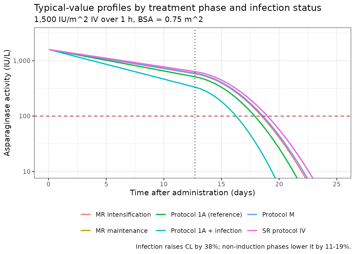
trough_at <- function(sc, tt = 14) {
  s <- filter(sim_tv, scenario == sc)
  s$Cc[which.min(abs(s$time - tt))]
}

scenario_covs |>
  transmute(
    Scenario = scenario,
    `CL multiplier (Kloos 2021 Table 2)` = c(1, 1.38, 0.87, 0.89, 0.81, 0.81),
    `Typical 14 day trough (IU/L)` = vapply(scenario, trough_at, numeric(1))
  ) |>
  knitr::kable(
    digits  = 2,
    caption = paste(
      "Typical-value 14 day (biweekly) trough asparaginase activity by",
      "treatment phase and infection status, after a 1,500 IU/m^2 dose."
    )
)| Scenario | CL multiplier (Kloos 2021 Table 2) | Typical 14 day trough (IU/L) |
|---|---|---|
| Protocol 1A (reference) | 1.00 | 425.04 |
| Protocol 1A + infection | 1.38 | 257.10 |
| Protocol M | 0.87 | 504.80 |
| MR intensification | 0.89 | 491.62 |
| MR maintenance | 0.81 | 546.50 |
| SR protocol IV | 0.81 | 546.50 |
Kloos 2021’s Clinical implications advise increasing the dose by 38% during an infection, if clinically possible; the infection row above shows the trough reduction that advice compensates for.
PKNCA validation
Non-compartmental analysis of the single-dose simulation. Two intervals are used, chosen to respect the split point:
-
0-12.7 days – the constant-clearance window. Here
the profile is a clean mono-exponential after the infusion ends, so the
NCA terminal half-life must reproduce the closed-form
ln(2) * Vd / CL. This is the strict check. -
0-14 days – the full biweekly dosing interval,
giving
Cmax,Tmax,AUCand the clinically relevant trough.
Subjects are grouped into BSA bands so per-group results can be
compared. The concentration frame is filtered only on
!is.na(Cc) so the time-zero record is retained.
pop_band <- pop |>
  mutate(
    bsa_band = case_when(
      BSA <  0.65             ~ "Low (<0.65 m^2)",
      BSA >= 0.65 & BSA < 1.05 ~ "Mid (0.65-1.05 m^2)",
      BSA >= 1.05             ~ "High (>=1.05 m^2)"
    ),
    bsa_band = factor(bsa_band, levels = c("Low (<0.65 m^2)",
                                           "Mid (0.65-1.05 m^2)",
                                           "High (>=1.05 m^2)"))
  )

nca_conc <- sim |>
  filter(!is.na(Cc)) |>
  left_join(select(pop_band, id, bsa_band), by = "id") |>
  transmute(id, time, Cc, treatment = bsa_band)

nca_dose <- doses |>
  left_join(select(pop_band, id, bsa_band), by = "id") |>
  transmute(id, time, amt, treatment = bsa_band)

conc_obj <- PKNCA::PKNCAconc(nca_conc, Cc ~ time | treatment + id,
                             concu = "IU/L", timeu = "day")
dose_obj <- PKNCA::PKNCAdose(nca_dose, amt ~ time | treatment + id,
                             doseu = "IU")

intervals <- data.frame(
  start     = c(0,    0),
  end       = c(12.7, 14),
  cmax      = c(TRUE, FALSE),
  tmax      = c(TRUE, FALSE),
  half.life = c(TRUE, FALSE),
  auclast   = c(FALSE, TRUE),
  ctrough   = c(FALSE, TRUE)
)

nca_res <- PKNCA::pk.nca(
  PKNCA::PKNCAdata(conc_obj, dose_obj, intervals = intervals)
)
keep_params <- c("cmax", "tmax", "half.life", "auclast", "ctrough")

nca_tab <- as.data.frame(nca_res) |>
  filter(PPTESTCD %in% keep_params) |>
  group_by(treatment, PPTESTCD) |>
  summarise(median = median(PPORRES, na.rm = TRUE), .groups = "drop")

nca_tab |>
  tidyr::pivot_wider(names_from = PPTESTCD, values_from = median) |>
  dplyr::rename(
    "BSA band"                 = treatment,
    "Cmax (IU/L)"              = cmax,
    "Tmax (days)"              = tmax,
    "t1/2, 0-12.7 d (days)"    = half.life,
    "AUC0-14d (IU*day/L)"      = auclast,
    "Trough at 14 d (IU/L)"    = ctrough
  ) |>
  knitr::kable(
    digits  = 2,
    caption = paste(
      "PKNCA summary (median per BSA band) after a single 1,500 IU/m^2",
      "PEGasparaginase infusion, protocol 1A, no infection."
    )
)| BSA band | AUC0-14d (IU*day/L) | Cmax (IU/L) | Trough at 14 d (IU/L) | t1/2, 0-12.7 d (days) | Tmax (days) |
|---|---|---|---|---|---|
| Low (<0.65 m^2) | 12015.44 | 1561.11 | 379.61 | 7.41 | 0.04 |
| Mid (0.65-1.05 m^2) | 12983.78 | 1657.95 | 401.87 | 7.49 | 0.04 |
| High (>=1.05 m^2) | 13465.29 | 1700.44 | 446.78 | 7.84 | 0.04 |
Comparison against the model’s closed-form expectations
Kloos 2021 publishes no NCA table, so the reference values below are
the closed-form predictions of the published parameters.
Cmax is
dose / Vd = 1500 * BSA / (0.94 * BSA) = 1596 IU/L (BSA
cancels, so it is the same in every band), and the terminal half-life
over the constant-CL window is ln(2) * 0.94 / 0.084 = 7.76
days (also BSA-independent). Agreement across BSA bands is itself a
check that the linear BSA normalization of both CL and Vd is encoded
correctly.
published <- tidyr::crossing(
  treatment = levels(pop_band$bsa_band),
  tibble(
    PPTESTCD = c("cmax", "half.life"),
    PPORRES  = c(dose_iu_per_m2 / 0.94, log(2) * 0.94 / 0.084)
  )
)

cmp <- nlmixr2lib::ncaComparisonTable(
  simulated     = nca_res,
  reference     = published,
  by            = "treatment",
  units         = c(cmax = "IU/L", half.life = "day"),
  tolerance_pct = 20
)

knitr::kable(
  cmp,
  caption = paste(
    "Simulated NCA versus the closed-form prediction from the Kloos 2021",
    "final-model parameters. * marks rows differing by >20%."
  )
)| NCA parameter | treatment | Reference | Simulated | % diff |
|---|---|---|---|---|
| Cmax (IU/L) | High (>=1.05 m^2) | 1600 | 1700 | +6.6% |
| Cmax (IU/L) | Low (<0.65 m^2) | 1600 | 1560 | -2.2% |
| Cmax (IU/L) | Mid (0.65-1.05 m^2) | 1600 | 1660 | +3.9% |
| t½ (day) | High (>=1.05 m^2) | 7.76 | 7.84 | +1.1% |
| t½ (day) | Low (<0.65 m^2) | 7.76 | 7.41 | -4.5% |
| t½ (day) | Mid (0.65-1.05 m^2) | 7.76 | 7.49 | -3.5% |
Kloos 2021 Table 4 starting-dose guideline
Table 4 recommends, for protocol 1A induction targeting a trough asparaginase activity of 100 IU/L, a loading dose of 800 IU/m^2 followed by a biweekly maintenance dose of 600 IU/m^2. The authors derived these by Monte Carlo simulation of 2,000 virtual patients, choosing the dose that gives adequate troughs in 95% of patients. The check below repeats that logic on the virtual cohort.
make_events <- function(load_iu_m2, maint_iu_m2, n_maint = 3) {
  dose_days <- seq(0, by = 14, length.out = n_maint + 1)
  amt_m2    <- c(load_iu_m2, rep(maint_iu_m2, n_maint))

  d <- tidyr::crossing(pop, tibble(dose_idx = seq_along(dose_days))) |>
    mutate(
      time = dose_days[dose_idx],
      amt  = amt_m2[dose_idx] * BSA,
      dur  = infusion_dur_d,
      evid = 1L,
      cmt  = "central",
      OCC  = pmin(dose_idx, 3L)
    ) |>
    select(-dose_idx)

  # Trough = immediately before each subsequent dose, plus the final trough.
  o <- tidyr::crossing(pop, tibble(time = dose_days + 14 - 1e-4)) |>
    mutate(amt = NA_real_, dur = NA_real_, evid = 0L, cmt = "central",
           OCC = pmin(findInterval(time, dose_days), 3L))

  bind_rows(d, o) |>
    mutate(DIS_INFECT_ACTIVE = 0L, TRTPH_1B = 0L, TRTPH_M = 0L,
           TRTPH_MR_INTENS = 0L, TRTPH_MR_MAINT = 0L, TRTPH_SR_IV = 0L) |>
    arrange(id, time, desc(evid)) |>
    as.data.frame()
}

ev_t4  <- make_events(800, 600)
sim_t4 <- rxode2::rxSolve(mod, ev_t4, omega = om,
                          keep = "BSA", returnType = "data.frame")
stopifnot(dplyr::n_distinct(sim_t4$id) == n_subj)

troughs <- sim_t4 |>
  filter(!is.na(Cc)) |>
  mutate(dose_number = findInterval(time, seq(0, by = 14, length.out = 4)))

troughs |>
  group_by(dose_number) |>
  summarise(
    `Median trough (IU/L)`   = median(Cc),
    `5th percentile (IU/L)`  = quantile(Cc, 0.05),
    `% >= 100 IU/L`          = 100 * mean(Cc >= 100),
    .groups = "drop"
  ) |>
  dplyr::rename("Dose number" = dose_number) |>
  knitr::kable(
    digits  = 1,
    caption = paste(
      "Trough asparaginase activity 14 days after each dose under the",
      "Kloos 2021 Table 4 protocol-1A regimen (800 IU/m^2 loading,",
      "600 IU/m^2 biweekly maintenance), target trough 100 IU/L."
    )
)| Dose number | Median trough (IU/L) | 5th percentile (IU/L) | % >= 100 IU/L |
|---|---|---|---|
| 1 | 216.9 | 125.2 | 97.5 |
| 2 | 221.8 | 119.4 | 99.0 |
| 3 | 234.9 | 119.1 | 97.5 |
| 4 | 238.7 | 105.8 | 97.0 |
Kloos 2021 chose these doses so that at least 95% of patients achieve the target; the simulated attainment above should be at or above that level. The 5th percentile is the quantity the authors’ 95%-attainment criterion constrains, so it is reported alongside the median.
Errata
The 2023 erratum (Haematologica 108(9):2558, doi:10.3324/haematol.2023.283685) corrects two typographical errors in the dose-adjustment nomogram of Table 5 of the original article:
- Target trough 100-250 IU/L column: the second “Week level” range is 100-150 IU/L, not 100-250 IU/L.
- Target trough 250-400 IU/L column: the third “Week level” range is 300-350 IU/L, not 300-250 IU/L.
Table 5 is a clinical dose-adjustment nomogram, not a source of model
parameters, so neither correction changes any value in
ini(). It is recorded here, and in the model file’s
reference field, because the erratum is this model’s
nominal lead document and because it demonstrates that the paper’s
tables are not error-free – which is directly relevant to the
additive-versus-multiplicative slope decision discussed above.
Assumptions and deviations
-
The time-dependent-clearance slope is implemented as
ADDITIVE, deviating from the two printed equations. Kloos 2021
Table 2’s final-model footer and the Online Supplementary Appendix both
print the multiplicative form
Cl_ind = 1 + Theta2 * (TAD - split point). This model implementsCL = Theta1 + Theta2 * (TAD - split point)instead. The evidence is set out in full in “The additive-slope reading” above: the parameter’s stated units (L/day/m^2/day), three separate prose statements, the three published structural-model half-lives (reproduced exactly by the additive reading, missed by 1.9-2.7x by the multiplicative one), and the “several days” convergence to native-asparaginase clearance (~5 days additive versus ~61 days multiplicative). Equivalently, the additive form is the supplement’s own equation withTheta2expressed relative toTheta1– i.e. treating the printed equation as missing a/ Theta1. This reading was ratified by the maintainers before drafting. - Individual baseline covariates are not published. The virtual cohort’s BSA distribution is a log-normal matched to the published median and IQR and clipped to the 0.52-2.3 m^2 range used in the authors’ own simulations. Age, weight and sex are not model covariates and are not simulated.
-
Inter-occasion variability uses three occasions.
The supplement defines an occasion as “administration of a new dose” but
does not fix a count. Three occasions are instantiated, matching the
three fixed 1,500 IU/m^2 induction doses of protocols 1A and 1B
(Supplemental Table 1). Records with
OCCoutside 1-3 receive no IOV contribution, so longer individualized-dosing simulations should either extend the occasion set or accept IIV-only variability beyond the third dose. -
Protocol 1B is encoded as
fixed(1), not dropped. Kloos 2021 could not estimate the 1B effect (only two high-risk patients) and fixed it to the 1A reference. Keeping the column preserves the provenance of that decision; numerically it is identical to omitting it. -
The volume of distribution has no independent eta.
IIV on Vd was not estimable because it correlated completely with the
CL-Vd correlation (Supplement, Supplemental Results). The CL eta is
shared and scaled by 1.26 per the supplement’s
Vd = Theta3 * e^(Theta4 * eta) * BSA. The main article’s Table 2 prints this equation without theBSAterm, which is dimensionally impossible for a parameter reported in L/m^2; the supplement settles it and is followed here. -
Doxorubicin and methotrexate are not covariates.
Both were significant in the univariate analysis and were evaluated in
the multivariate analysis on clinical grounds, but neither survived
backward elimination (Kloos 2021 Results, Covariate analysis). They are
documented in
covariatesDataExcludedrather thancovariateData, along with leukocytes, creatinine and anti-asparaginase antibodies. - Values below the assay LLQ (10 IU/L) were excluded by the authors. The simulations here are not censored at the LLQ, so simulated late-time activity levels can fall below values the original analysis would have discarded.
-
Time after dose is evaluated inside the ODE, not as a
model-block local. rxode2 evaluates the standalone algebraic
assignments of
model()once per output record and holds them constant across the integration interval, so a clearance built from atad()local becomes a step function of the observation grid: for a single trough observation 14 days after an 800 IU/m^2 dose that yields 50 IU/L, versus 227 IU/L on a dense grid. The model file therefore writes the time-after-dose term inline in thed/dt(central)right-hand side ast - tlast(), which rxode2 evaluates at every solver step, making the solution exact and independent of the output grid. Thecl,cl_indandkelsolve columns are record-level reporting copies and do not feed the ODE. Users building their own event tables need no special grid density. - The paper reports no NCA parameters. The PKNCA comparison table therefore uses closed-form predictions from the published parameter values as its reference, not published NCA results.
Reference
Kloos RQH, Mathot R, Pieters R, van der Sluis IM. Individualized dosing guidelines for PEGasparaginase and factors influencing the clearance: a population pharmacokinetic model. Haematologica. 2021;106(5):1254-1261. doi:10.3324/haematol.2019.242289
Erratum. Haematologica. 2023;108(9):2558. doi:10.3324/haematol.2023.283685