Olanzapine (Zhang 2024)
Source:vignettes/articles/Zhang_2024_olanzapine.Rmd
Zhang_2024_olanzapine.RmdModel and source
- Citation: Zhang C, Jiang L, Hu K, Chen L, Zhang YJ, Shi HZ, He SM, Chen X, Wang DD. Effects of Aripiprazole on Olanzapine Population Pharmacokinetics and Initial Dosage Optimization in Schizophrenia Patients. Neuropsychiatric Disease and Treatment. 2024;20:479-490. doi:10.2147/NDT.S455183. Final model Equations (6) and (7); parameter estimates Table 3. The fixed absorption rate constant is quoted from the paper’s reference 29: Sun L, Mills R, Sadler BM, Rege B. Population pharmacokinetics of olanzapine and samidorphan when administered in combination in healthy subjects and patients with schizophrenia. J Clin Pharmacol. 2021;61(11):1430-1441. doi:10.1002/jcph.1911.
- Description: One-compartment population PK model for oral olanzapine with first-order absorption in adults with schizophrenia, built from a routine therapeutic-drug-monitoring database (Zhang 2024). Apparent oral clearance is allometrically scaled on body weight and reduced by 39.2% when aripiprazole is co-administered; the absorption rate constant is fixed to a published value. Between-subject variability was retained on CL/F only.
- Article: https://doi.org/10.2147/NDT.S455183
Zhang and colleagues fitted a one-compartment model with first-order oral absorption to routine therapeutic-drug-monitoring (TDM) concentrations from 65 inpatients with schizophrenia. The absorption rate constant was not identifiable from sparse trough-dominated TDM data and was fixed to a published value; apparent oral clearance and apparent volume were estimated. Of the 30 concomitant medications screened, only aripiprazole was retained: patients co-prescribed aripiprazole had 39.2% lower olanzapine CL/F.
Population
Sixty-five inpatients with schizophrenia treated at a single centre in Xuzhou, Jiangsu, China contributed olanzapine TDM concentrations collected between July 2020 and October 2022 (Methods, Data Collection). The cohort was 36 men and 29 women, mean age 45.92 years (SD 15.79) and mean weight 63.16 kg (SD 10.57) (Table 1). Baseline laboratory values were broadly unremarkable: mean albumin 41.53 g/L, creatinine 66.16 umol/L, alanine transaminase 23.52 IU/L. Four of the 65 patients were co-prescribed aripiprazole orally disintegrating tablets (Table 2).
The paper reports no administered olanzapine doses, dose ranges, or sampling times; the concentrations come from a routine TDM database rather than a designed PK study. Every dosing regimen used below is therefore a scenario constructed for validation, not a replication of the observed data.
The same information is available programmatically via the model’s
population metadata
(readModelDb("Zhang_2024_olanzapine")()$population).
Source trace
The per-parameter origin is recorded as an in-file comment next to
each ini() entry in
inst/modeldb/specificDrugs/Zhang_2024_olanzapine.R. The
table below collects them in one place.
| Equation / parameter | Value | Source location |
|---|---|---|
lcl (CL/F at 70 kg, no aripiprazole) |
27.6 L/h | Table 3 (SE 5.6%; bootstrap median 27.3 [24.7, 30.4]); also printed in Equation (6) and restated in the Discussion |
lvc (V/F at 70 kg) |
854 L | Table 3 (SE 25.5%; bootstrap median 858 [600, 2530]); also printed in Equation (7) and restated in the Discussion |
lka (ka, fixed) |
0.861 1/h | Table 3, “0.861 (fixed)”; Methods, Modeling: “absorption rate constant (Ka, fixed at 0.861/h[29])”. Reference 29 is Sun 2021, J Clin Pharmacol 61(11):1430-1441 |
e_wt_cl (allometric exponent on CL/F, fixed) |
0.75 | Methods, Equation (3): “Z represented the allometric coefficient: 0.75 for the CL/F and 1 for the V/F”, citing Anderson & Holford 2008; the exponent is printed again in Equation (6) |
e_wt_vc (allometric exponent on V/F, fixed) |
1 | Methods, Equation (3); printed again in Equation (7) |
e_ari_cl (concomitant aripiprazole on CL/F) |
-0.392 | Table 3, theta_ARI (SE 27.8%; bootstrap median -0.377 [-0.535,
-0.194]); assembled in Equation (6) as
(1 - 0.392 * ARI)
|
etalcl (IIV on CL/F) |
omega = 0.316, so variance 0.316^2 | Table 3, row omega_CL/F (SE 13.4%; bootstrap median
0.321 [0.223, 0.395]). Read as a standard deviation – see Assumptions
below |
propSd (proportional residual error) |
0.288 | Table 3, row sigma_1, “residual variability,
proportional error” (SE 10.1%) |
addSd (additive residual error) |
3.701 ng/mL | Table 3, row sigma_2, “residual variability, additive
error” (SE 17.4%) |
IIV structure L_i = TV(L) * exp(eta_i)
|
n/a | Methods, Equation (1) |
Residual structure T_i = U_i + U_i*eps_1 + eps_2
|
n/a | Methods, Equation (2) |
Allometry V_i = V_std * (Y_i / Y_std)^Z,
Y_std = 70 kg
|
n/a | Methods, Equation (3) |
| Categorical covariate form (linear shift) | n/a | Methods, Equation (5); realised in Equation (6) |
CL/F = 27.6 * (weight/70)^0.75 * (1 - 0.392 * ARI) |
n/a | Results, Modeling, Equation (6) |
V/F = 854 * (weight/70) |
n/a | Results, Modeling, Equation (7) |
| Therapeutic range 20-80 ng/mL | n/a | Methods, Simulation (cites the paper’s reference 16, Ding 2022) |
| Initial-dose recommendations | n/a | Table 4 and Figure 4 |
mod <- readModelDb("Zhang_2024_olanzapine")
ui  <- rxode2::rxode(mod)
#> ℹ parameter labels from comments will be replaced by 'label()'
Structural checks against the printed equations
The published model is fully specified by Equations (6) and (7), so
the first check is that the packaged model reproduces them exactly.
zeroRe() removes between-subject variability so the solved
cl and vc are the typical values.
# Published equations, transcribed independently of the model file.
cl_published <- function(wt, ari) 27.6 * (wt / 70)^0.75 * (1 - 0.392 * ari)
vc_published <- function(wt)      854  * (wt / 70)

grid <- tidyr::expand_grid(WT = c(40, 50, 60, 70, 80, 90, 100),
                           CONMED_ARIPIPRAZOLE = c(0, 1)) |>
  dplyr::mutate(id = dplyr::row_number(),
                arm = paste0(WT, " kg, ",
                             ifelse(CONMED_ARIPIPRAZOLE == 1, "with", "no"),
                             " aripiprazole"))

ev_struct <- grid |>
  dplyr::mutate(time = 0, amt = 10, evid = 1, cmt = "depot") |>
  dplyr::bind_rows(
    grid |> tidyr::crossing(time = 0:1) |>
      dplyr::mutate(amt = NA_real_, evid = 0, cmt = "central")
  ) |>
  dplyr::arrange(id, time, dplyr::desc(evid))

sim_struct <- rxode2::rxSolve(
  rxode2::zeroRe(mod), events = ev_struct,
  keep = c("WT", "CONMED_ARIPIPRAZOLE", "arm")
) |>
  as.data.frame() |>
  dplyr::group_by(WT, CONMED_ARIPIPRAZOLE, arm) |>
  dplyr::summarise(cl_model = mean(cl), vc_model = mean(vc), ka_model = mean(ka),
                   .groups = "drop") |>
  dplyr::mutate(cl_paper = cl_published(WT, CONMED_ARIPIPRAZOLE),
                vc_paper = vc_published(WT))
#> ℹ parameter labels from comments will be replaced by 'label()'
#> ℹ omega/sigma items treated as zero: 'etalcl'
#> Warning: multi-subject simulation without without 'omega'

stopifnot(
  nrow(sim_struct) == 14L,
  max(abs(sim_struct$cl_model - sim_struct$cl_paper)) < 1e-8,
  max(abs(sim_struct$vc_model - sim_struct$vc_paper)) < 1e-8,
  max(abs(sim_struct$ka_model - 0.861)) < 1e-8
)

sim_struct |>
  dplyr::transmute(
    Arm                 = arm,
    `CL/F model (L/h)`  = round(cl_model, 3),
    `CL/F Eq. 6 (L/h)`  = round(cl_paper, 3),
    `V/F model (L)`     = round(vc_model, 1),
    `V/F Eq. 7 (L)`     = round(vc_paper, 1)
  ) |>
knitr::kable(caption = "Typical CL/F and V/F reproduce Equations (6) and (7) exactly.")| Arm | CL/F model (L/h) | CL/F Eq. 6 (L/h) | V/F model (L) | V/F Eq. 7 (L) |
|---|---|---|---|---|
| 40 kg, no aripiprazole | 18.140 | 18.140 | 488 | 488 |
| 40 kg, with aripiprazole | 11.029 | 11.029 | 488 | 488 |
| 50 kg, no aripiprazole | 21.444 | 21.444 | 610 | 610 |
| 50 kg, with aripiprazole | 13.038 | 13.038 | 610 | 610 |
| 60 kg, no aripiprazole | 24.587 | 24.587 | 732 | 732 |
| 60 kg, with aripiprazole | 14.949 | 14.949 | 732 | 732 |
| 70 kg, no aripiprazole | 27.600 | 27.600 | 854 | 854 |
| 70 kg, with aripiprazole | 16.781 | 16.781 | 854 | 854 |
| 80 kg, no aripiprazole | 30.507 | 30.507 | 976 | 976 |
| 80 kg, with aripiprazole | 18.548 | 18.548 | 976 | 976 |
| 90 kg, no aripiprazole | 33.325 | 33.325 | 1098 | 1098 |
| 90 kg, with aripiprazole | 20.261 | 20.261 | 1098 | 1098 |
| 100 kg, no aripiprazole | 36.065 | 36.065 | 1220 | 1220 |
| 100 kg, with aripiprazole | 21.928 | 21.928 | 1220 | 1220 |
The Discussion and Figure 1H state the aripiprazole effect as a
clearance ratio: “at the same weight, the olanzapine clearance rates
were 0.608:1 in patients with or without aripiprazole”. That ratio is
1 - 0.392 and is weight-independent, so it must hold at
every weight.
ratio <- sim_struct |>
  dplyr::select(WT, CONMED_ARIPIPRAZOLE, cl_model) |>
  tidyr::pivot_wider(names_from = CONMED_ARIPIPRAZOLE,
                     names_prefix = "ari", values_from = cl_model) |>
  dplyr::mutate(ratio = ari1 / ari0)

# Deterministic (no IIV): an exact identity, so a tight bound is correct here.
stopifnot(nrow(ratio) == 7L, max(abs(ratio$ratio - 0.608)) < 1e-9)

ratio |>
  dplyr::transmute(`Weight (kg)` = WT,
                   `CL/F without aripiprazole (L/h)` = round(ari0, 2),
                   `CL/F with aripiprazole (L/h)`    = round(ari1, 2),
                   `Ratio (with:without)`            = round(ratio, 4)) |>
knitr::kable(caption = "Replicates Figure 1H of Zhang 2024: a clearance ratio of 0.608:1 with vs without aripiprazole, at every weight.")| Weight (kg) | CL/F without aripiprazole (L/h) | CL/F with aripiprazole (L/h) | Ratio (with:without) |
|---|---|---|---|
| 40 | 18.14 | 11.03 | 0.608 |
| 50 | 21.44 | 13.04 | 0.608 |
| 60 | 24.59 | 14.95 | 0.608 |
| 70 | 27.60 | 16.78 | 0.608 |
| 80 | 30.51 | 18.55 | 0.608 |
| 90 | 33.32 | 20.26 | 0.608 |
| 100 | 36.06 | 21.93 | 0.608 |
PKNCA validation against the published parameters
Zhang 2024 reports no NCA table, but the printed structural parameters imply exact non-compartmental quantities for a single oral dose of a linear one-compartment model:
-
AUC0-inf = Dose / (CL/F)(mass balance; independent ofkaandV/F), - terminal
t1/2 = ln(2) * (V/F) / (CL/F), becauseka = 0.861 1/his far larger thankel(0.032 1/h without aripiprazole, 0.020 1/h with), so the terminal phase is elimination-rate-limited rather than flip-flop, -
tmax = ln(ka / kel) / (ka - kel).
Running PKNCA over a typical-value (no-IIV) simulation therefore checks the whole pipeline – units, the mg-to-ng/mL conversion, the ODE system, the covariate model – against numbers derived from Table 3 alone.
# Single 10 mg oral dose; observe long enough for AUC0-inf to converge.
# t1/2 with aripiprazole is ~35 h, so 720 h is >20 half-lives.
obs_times <- sort(unique(c(seq(0, 24, by = 0.1), seq(24, 720, by = 1))))

ev_nca <- grid |>
  dplyr::mutate(time = 0, amt = 10, evid = 1, cmt = "depot") |>
  dplyr::bind_rows(
    grid |> tidyr::crossing(time = obs_times) |>
      dplyr::mutate(amt = NA_real_, evid = 0, cmt = "central")
  ) |>
  dplyr::arrange(id, time, dplyr::desc(evid))

stopifnot(!anyDuplicated(unique(ev_nca[, c("id", "time", "evid")])))

sim_nca_raw <- rxode2::rxSolve(
  rxode2::zeroRe(mod), events = ev_nca,
  keep = c("WT", "CONMED_ARIPIPRAZOLE", "arm")
) |>
  as.data.frame()
#> ℹ parameter labels from comments will be replaced by 'label()'
#> ℹ omega/sigma items treated as zero: 'etalcl'
#> Warning: multi-subject simulation without without 'omega'

# Concentrations must stay non-negative for PKNCA's log-linear terminal fit.
stopifnot(all(sim_nca_raw$Cc >= 0, na.rm = TRUE))
sim_nca <- sim_nca_raw |>
  dplyr::filter(!is.na(Cc)) |>
  dplyr::select(id, time, Cc, arm)

# Guarantee a time = 0 row per (id, arm); pre-dose Cc = 0 for extravascular.
sim_nca <- dplyr::bind_rows(
  sim_nca,
  sim_nca |> dplyr::distinct(id, arm) |> dplyr::mutate(time = 0, Cc = 0)
) |>
  dplyr::distinct(id, arm, time, .keep_all = TRUE) |>
  dplyr::arrange(id, arm, time)

conc_obj <- PKNCA::PKNCAconc(sim_nca, Cc ~ time | arm + id,
                             concu = "ng/mL", timeu = "h")

dose_df <- ev_nca |>
  dplyr::filter(evid == 1) |>
  dplyr::select(id, time, amt, arm)

dose_obj <- PKNCA::PKNCAdose(dose_df, amt ~ time | arm + id, doseu = "mg")

intervals <- data.frame(
  start      = 0,
  end        = Inf,
  cmax       = TRUE,
  tmax       = TRUE,
  aucinf.obs = TRUE,
  half.life  = TRUE
)

nca_res <- PKNCA::pk.nca(PKNCA::PKNCAdata(conc_obj, dose_obj, intervals = intervals))
Comparison against the values implied by Table 3
# Reference values derived from the PRINTED parameters only.
ka_pub <- 0.861
published <- grid |>
  dplyr::mutate(
    cl  = cl_published(WT, CONMED_ARIPIPRAZOLE),
    vc  = vc_published(WT),
    kel = cl / vc,
    # 10 mg / (L/h) -> mg*h/L; * 1000 -> ng*h/mL
    aucinf.obs = 1000 * 10 / cl,
    half.life  = log(2) / kel,
    tmax       = log(ka_pub / kel) / (ka_pub - kel),
    cmax       = 1000 * (10 / vc) * (ka_pub / (ka_pub - kel)) *
      (exp(-kel * tmax) - exp(-ka_pub * tmax))
  ) |>
  dplyr::select(arm, cmax, tmax, aucinf.obs, half.life)

cmp <- nlmixr2lib::ncaComparisonTable(
  simulated     = nca_res,
  reference     = published,
  by            = "arm",
  units         = c(cmax = "ng/mL", tmax = "h",
                    aucinf.obs = "ng*h/mL", half.life = "h"),
  tolerance_pct = 20
)

knitr::kable(
  cmp,
  caption = paste(
    "Simulated NCA vs the closed-form values implied by Zhang 2024 Table 3",
    "(10 mg single oral dose). * marks a >20% difference."
  )
)| NCA parameter | arm | Reference | Simulated | % diff |
|---|---|---|---|---|
| Cmax (ng/mL) | 40 kg, no aripiprazole | 17.8 | 17.8 | -0.0% |
| Cmax (ng/mL) | 40 kg, with aripiprazole | 18.6 | 18.6 | -0.0% |
| Cmax (ng/mL) | 50 kg, no aripiprazole | 14.3 | 14.3 | -0.0% |
| Cmax (ng/mL) | 50 kg, with aripiprazole | 14.9 | 14.9 | -0.0% |
| Cmax (ng/mL) | 60 kg, no aripiprazole | 12 | 12 | -0.0% |
| Cmax (ng/mL) | 60 kg, with aripiprazole | 12.5 | 12.5 | -0.0% |
| Cmax (ng/mL) | 70 kg, no aripiprazole | 10.3 | 10.3 | -0.0% |
| Cmax (ng/mL) | 70 kg, with aripiprazole | 10.7 | 10.7 | -0.0% |
| Cmax (ng/mL) | 80 kg, no aripiprazole | 9.04 | 9.04 | -0.0% |
| Cmax (ng/mL) | 80 kg, with aripiprazole | 9.4 | 9.4 | -0.0% |
| Cmax (ng/mL) | 90 kg, no aripiprazole | 8.06 | 8.06 | -0.0% |
| Cmax (ng/mL) | 90 kg, with aripiprazole | 8.37 | 8.37 | -0.0% |
| Cmax (ng/mL) | 100 kg, no aripiprazole | 7.27 | 7.27 | -0.0% |
| Cmax (ng/mL) | 100 kg, with aripiprazole | 7.55 | 7.55 | -0.0% |
| Tmax (h) | 40 kg, no aripiprazole | 3.81 | 3.8 | -0.4% |
| Tmax (h) | 40 kg, with aripiprazole | 4.34 | 4.3 | -1.0% |
| Tmax (h) | 50 kg, no aripiprazole | 3.87 | 3.9 | +0.7% |
| Tmax (h) | 50 kg, with aripiprazole | 4.4 | 4.4 | -0.0% |
| Tmax (h) | 60 kg, no aripiprazole | 3.92 | 3.9 | -0.5% |
| Tmax (h) | 60 kg, with aripiprazole | 4.45 | 4.5 | +1.1% |
| Tmax (h) | 70 kg, no aripiprazole | 3.96 | 4 | +1.0% |
| Tmax (h) | 70 kg, with aripiprazole | 4.49 | 4.5 | +0.2% |
| Tmax (h) | 80 kg, no aripiprazole | 4 | 4 | +0.1% |
| Tmax (h) | 80 kg, with aripiprazole | 4.53 | 4.5 | -0.6% |
| Tmax (h) | 90 kg, no aripiprazole | 4.03 | 4 | -0.7% |
| Tmax (h) | 90 kg, with aripiprazole | 4.56 | 4.6 | +0.9% |
| Tmax (h) | 100 kg, no aripiprazole | 4.06 | 4.1 | +1.1% |
| Tmax (h) | 100 kg, with aripiprazole | 4.59 | 4.6 | +0.2% |
| AUC0-∞ (obs) (ng*h/mL) | 40 kg, no aripiprazole | 551 | 551 | -0.0% |
| AUC0-∞ (obs) (ng*h/mL) | 40 kg, with aripiprazole | 907 | 907 | -0.0% |
| AUC0-∞ (obs) (ng*h/mL) | 50 kg, no aripiprazole | 466 | 466 | -0.0% |
| AUC0-∞ (obs) (ng*h/mL) | 50 kg, with aripiprazole | 767 | 767 | -0.0% |
| AUC0-∞ (obs) (ng*h/mL) | 60 kg, no aripiprazole | 407 | 407 | -0.0% |
| AUC0-∞ (obs) (ng*h/mL) | 60 kg, with aripiprazole | 669 | 669 | -0.0% |
| AUC0-∞ (obs) (ng*h/mL) | 70 kg, no aripiprazole | 362 | 362 | -0.0% |
| AUC0-∞ (obs) (ng*h/mL) | 70 kg, with aripiprazole | 596 | 596 | -0.0% |
| AUC0-∞ (obs) (ng*h/mL) | 80 kg, no aripiprazole | 328 | 328 | -0.0% |
| AUC0-∞ (obs) (ng*h/mL) | 80 kg, with aripiprazole | 539 | 539 | -0.0% |
| AUC0-∞ (obs) (ng*h/mL) | 90 kg, no aripiprazole | 300 | 300 | -0.0% |
| AUC0-∞ (obs) (ng*h/mL) | 90 kg, with aripiprazole | 494 | 494 | -0.0% |
| AUC0-∞ (obs) (ng*h/mL) | 100 kg, no aripiprazole | 277 | 277 | -0.0% |
| AUC0-∞ (obs) (ng*h/mL) | 100 kg, with aripiprazole | 456 | 456 | -0.0% |
| t½ (h) | 40 kg, no aripiprazole | 18.6 | 18.7 | +0.0% |
| t½ (h) | 40 kg, with aripiprazole | 30.7 | 30.7 | +0.0% |
| t½ (h) | 50 kg, no aripiprazole | 19.7 | 19.7 | +0.0% |
| t½ (h) | 50 kg, with aripiprazole | 32.4 | 32.4 | +0.0% |
| t½ (h) | 60 kg, no aripiprazole | 20.6 | 20.6 | +0.0% |
| t½ (h) | 60 kg, with aripiprazole | 33.9 | 33.9 | +0.0% |
| t½ (h) | 70 kg, no aripiprazole | 21.4 | 21.4 | +0.0% |
| t½ (h) | 70 kg, with aripiprazole | 35.3 | 35.3 | +0.0% |
| t½ (h) | 80 kg, no aripiprazole | 22.2 | 22.2 | +0.0% |
| t½ (h) | 80 kg, with aripiprazole | 36.5 | 36.5 | +0.0% |
| t½ (h) | 90 kg, no aripiprazole | 22.8 | 22.8 | +0.0% |
| t½ (h) | 90 kg, with aripiprazole | 37.6 | 37.6 | +0.0% |
| t½ (h) | 100 kg, no aripiprazole | 23.4 | 23.4 | +0.0% |
| t½ (h) | 100 kg, with aripiprazole | 38.6 | 38.6 | +0.0% |
# These are deterministic comparisons -- a typical-value solve against a closed
# form built from the paper's printed numbers -- so the residual difference is
# pure numerical (grid resolution, log-linear terminal fit) and a tight bound
# is correct. Contrast with the cohort-derived attainment table below.
nca_wide <- as.data.frame(nca_res$result) |>
  dplyr::select(arm, PPTESTCD, PPORRES) |>
  tidyr::pivot_wider(names_from = PPTESTCD, values_from = PPORRES) |>
  dplyr::left_join(published, by = "arm", suffix = c("_sim", "_pub"))

pct <- function(a, b) 100 * (a - b) / b
stopifnot(
  nrow(nca_wide) == 14L,
  max(abs(pct(nca_wide$aucinf.obs_sim, nca_wide$aucinf.obs_pub))) < 0.5,
  max(abs(pct(nca_wide$half.life_sim,  nca_wide$half.life_pub)))  < 0.5,
  max(abs(pct(nca_wide$cmax_sim,       nca_wide$cmax_pub)))       < 1.0,
  max(abs(pct(nca_wide$tmax_sim,       nca_wide$tmax_pub)))       < 2.0
)
AUC0-inf matches Dose / (CL/F) and the
terminal half-life matches ln(2) * (V/F) / (CL/F) to well
under 1%, confirming that the packaged model, its unit conversion and
its covariate model all agree with Table 3.
Replicate Figure 3: steady-state profiles at the recommended doses
Figure 3 of Zhang 2024 plots simulated olanzapine concentration-time profiles for seven weight groups under four conditions – once- or twice-daily dosing, with or without aripiprazole – against the 20-80 ng/mL therapeutic band. The panels below show the typical-value steady-state profile at the dose Table 4 recommends for each weight and condition.
# Table 4 of Zhang 2024, transcribed. Weight bands are inclusive of the lower
# bound; the paper's brackets overlap at the boundary weights, and the
# recommendation there is the lower-dose row.
recommended_dose <- function(wt, ari, ndose) {
  if (ari == 0 && ndose == 1) ifelse(wt < 70,  0.6, 0.5)
  else if (ari == 0 && ndose == 2) ifelse(wt < 60,  0.6, 0.5)
  else if (ari == 1 && ndose == 1) ifelse(wt < 53,  0.4, 0.3)
  else 0.4
}

conditions <- tidyr::expand_grid(
  CONMED_ARIPIPRAZOLE = c(0, 1),
  ndose               = c(1, 2),
  WT                  = c(40, 50, 60, 70, 80, 90, 100)
) |>
  dplyr::rowwise() |>
  dplyr::mutate(mg_per_kg_day = recommended_dose(WT, CONMED_ARIPIPRAZOLE, ndose)) |>
  dplyr::ungroup() |>
  dplyr::mutate(
    tau       = 24 / ndose,
    amt       = mg_per_kg_day * WT / ndose,
    condition = paste0(ifelse(ndose == 1, "Once daily", "Twice daily"), ", ",
                       ifelse(CONMED_ARIPIPRAZOLE == 1, "with", "no"),
                       " aripiprazole"),
    wt_label  = paste0(WT, " kg")
  )

conditions |>
  dplyr::transmute(Condition = condition, `Weight (kg)` = WT,
                   `Table 4 dose (mg/kg/day)` = mg_per_kg_day,
                   `Dose per administration (mg)` = round(amt, 1)) |>
knitr::kable(caption = "Recommended initial doses transcribed from Table 4 of Zhang 2024.")| Condition | Weight (kg) | Table 4 dose (mg/kg/day) | Dose per administration (mg) |
|---|---|---|---|
| Once daily, no aripiprazole | 40 | 0.6 | 24.0 |
| Once daily, no aripiprazole | 50 | 0.6 | 30.0 |
| Once daily, no aripiprazole | 60 | 0.6 | 36.0 |
| Once daily, no aripiprazole | 70 | 0.5 | 35.0 |
| Once daily, no aripiprazole | 80 | 0.5 | 40.0 |
| Once daily, no aripiprazole | 90 | 0.5 | 45.0 |
| Once daily, no aripiprazole | 100 | 0.5 | 50.0 |
| Twice daily, no aripiprazole | 40 | 0.6 | 12.0 |
| Twice daily, no aripiprazole | 50 | 0.6 | 15.0 |
| Twice daily, no aripiprazole | 60 | 0.5 | 15.0 |
| Twice daily, no aripiprazole | 70 | 0.5 | 17.5 |
| Twice daily, no aripiprazole | 80 | 0.5 | 20.0 |
| Twice daily, no aripiprazole | 90 | 0.5 | 22.5 |
| Twice daily, no aripiprazole | 100 | 0.5 | 25.0 |
| Once daily, with aripiprazole | 40 | 0.4 | 16.0 |
| Once daily, with aripiprazole | 50 | 0.4 | 20.0 |
| Once daily, with aripiprazole | 60 | 0.3 | 18.0 |
| Once daily, with aripiprazole | 70 | 0.3 | 21.0 |
| Once daily, with aripiprazole | 80 | 0.3 | 24.0 |
| Once daily, with aripiprazole | 90 | 0.3 | 27.0 |
| Once daily, with aripiprazole | 100 | 0.3 | 30.0 |
| Twice daily, with aripiprazole | 40 | 0.4 | 8.0 |
| Twice daily, with aripiprazole | 50 | 0.4 | 10.0 |
| Twice daily, with aripiprazole | 60 | 0.4 | 12.0 |
| Twice daily, with aripiprazole | 70 | 0.4 | 14.0 |
| Twice daily, with aripiprazole | 80 | 0.4 | 16.0 |
| Twice daily, with aripiprazole | 90 | 0.4 | 18.0 |
| Twice daily, with aripiprazole | 100 | 0.4 | 20.0 |
# 20 days of run-in reaches steady state: the slowest arm (with aripiprazole)
# has t1/2 = ln(2) * 854 / 16.78 = 35.3 h, so 480 h is >13 half-lives.
run_in_h <- 480

make_arm <- function(row, id) {
  tau  <- row$tau
  dose <- tibble::tibble(
    id = id, time = seq(0, run_in_h - tau, by = tau),
    amt = row$amt, evid = 1, cmt = "depot"
  )
  last_dose <- max(dose$time)
  obs <- tibble::tibble(
    id = id, time = seq(last_dose, last_dose + tau, by = tau / 96),
    amt = NA_real_, evid = 0, cmt = "central"
  )
  dplyr::bind_rows(dose, obs) |>
    dplyr::mutate(WT = row$WT,
                  CONMED_ARIPIPRAZOLE = row$CONMED_ARIPIPRAZOLE,
                  condition = row$condition, wt_label = row$wt_label,
                  tau = tau, t_rel = time - last_dose)
}

ev_fig3 <- do.call(
  dplyr::bind_rows,
  lapply(seq_len(nrow(conditions)),
         function(i) make_arm(conditions[i, ], id = i))
) |>
  dplyr::arrange(id, time, dplyr::desc(evid))

stopifnot(!anyDuplicated(unique(ev_fig3[, c("id", "time", "evid")])))
sim_fig3 <- rxode2::rxSolve(
  rxode2::zeroRe(mod), events = ev_fig3,
  keep = c("WT", "CONMED_ARIPIPRAZOLE", "condition", "wt_label")
) |>
  as.data.frame() |>
  dplyr::filter(!is.na(Cc)) |>
  dplyr::group_by(id) |>
  dplyr::mutate(t_rel = time - min(time)) |>
  dplyr::ungroup() |>
  dplyr::mutate(wt_label = factor(wt_label,
                                  levels = paste0(c(40, 50, 60, 70, 80, 90, 100), " kg")))
#> ℹ parameter labels from comments will be replaced by 'label()'
#> ℹ omega/sigma items treated as zero: 'etalcl'
#> Warning: multi-subject simulation without without 'omega'

ggplot(sim_fig3, aes(t_rel, Cc, colour = wt_label)) +
  geom_hline(yintercept = c(20, 80), linetype = "dashed", colour = "red") +
  geom_line() +
  facet_wrap(~condition) +
  labs(x = "Time within the steady-state dosing interval (h)",
       y = "Olanzapine concentration (ng/mL)",
       colour = "Body weight",
       title = "Steady-state profiles at the Table 4 recommended doses",
       caption = "Replicates the structure of Figure 3 of Zhang 2024; red dashed lines are the 20-80 ng/mL therapeutic range.")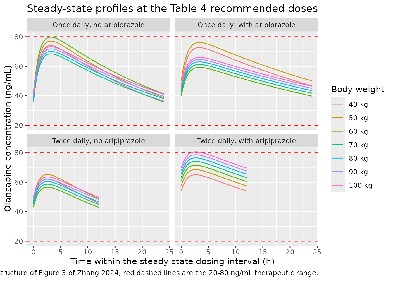
The typical-value profile lies inside the therapeutic band in 27 of the 28 arms. The single exception is the heaviest twice-daily arm with aripiprazole, whose peak reaches just over the 80 ng/mL ceiling.
band <- sim_fig3 |>
  dplyr::group_by(condition, wt_label) |>
  dplyr::summarise(cmin = min(Cc), cmax = max(Cc),
                   cav  = sum(diff(time) * (head(Cc, -1) + tail(Cc, -1)) / 2) /
                     (max(time) - min(time)),
                   .groups = "drop")

# Deterministic (zeroRe) typical-value profiles -- no cohort noise anywhere in
# this chunk, so tight bounds are correct here. A mis-transcribed dose,
# clearance, volume or unit conversion moves these by tens of percent.
over <- band |> dplyr::filter(cmax > 80)
stopifnot(
  nrow(band) == 28L,
  # Trough and interval-average are inside the therapeutic range everywhere.
  all(band$cmin >= 20),
  all(band$cav >= 20 & band$cav <= 80),
  # Exactly one arm's peak clears the ceiling, and only just.
  nrow(over) == 1L,
  over$condition == "Twice daily, with aripiprazole",
  over$wt_label == "100 kg",
  over$cmax < 82
)

band |>
  dplyr::filter(cmax > 78) |>
  dplyr::transmute(Condition = condition, Weight = wt_label,
                   `Ctrough (ng/mL)` = round(cmin, 1),
                   `Cav (ng/mL)`     = round(cav, 1),
                   `Cmax (ng/mL)`    = round(cmax, 1)) |>
knitr::kable(caption = "Arms whose typical steady-state peak approaches the 80 ng/mL ceiling.")| Condition | Weight | Ctrough (ng/mL) | Cav (ng/mL) | Cmax (ng/mL) |
|---|---|---|---|---|
| Once daily, no aripiprazole | 60 kg | 41.3 | 61 | 79.8 |
| Twice daily, with aripiprazole | 90 kg | 67.6 | 74 | 78.6 |
| Twice daily, with aripiprazole | 100 kg | 69.5 | 76 | 80.6 |
Target-attainment simulation (Table 4 and Figure 4)
Zhang 2024 simulated 1000 virtual patients per condition and reported “the probability for achieving target concentration” against the 20-80 ng/mL range (Methods, Simulation; results in Figure 4 and Table 4). The paper does not state which concentration the criterion is applied to – the trough, the average over the interval, or the entire profile – so the numbers below use the steady-state trough, the quantity a TDM service actually measures, and are presented for comparison rather than as a gate on the twice-daily arms. See Assumptions and deviations.
# rxSetSeed fixes rxode2's RNG per solver thread and NOT across thread counts,
# so this cohort differs between a 16-thread workstation and a 2-core CI
# runner. Every assertion below is written to hold for any such cohort.
rxode2::rxSetSeed(20240301)
n_per_arm <- 150L   # cap is 200 per arm

make_cohort_arm <- function(row, id_offset) {
  tau  <- row$tau
  ids  <- id_offset + seq_len(n_per_arm)
  dose <- tidyr::expand_grid(id = ids, time = seq(0, run_in_h - tau, by = tau)) |>
    dplyr::mutate(amt = row$amt, evid = 1, cmt = "depot")
  last_dose <- run_in_h - tau
  obs <- tidyr::expand_grid(id = ids,
                            time = seq(last_dose, last_dose + tau, by = tau / 48)) |>
    dplyr::mutate(amt = NA_real_, evid = 0, cmt = "central")
  dplyr::bind_rows(dose, obs) |>
    dplyr::mutate(WT = row$WT, CONMED_ARIPIPRAZOLE = row$CONMED_ARIPIPRAZOLE,
                  condition = row$condition, wt_label = row$wt_label) |>
    dplyr::arrange(id, time, dplyr::desc(evid))
}

# One rxSolve call per condition keeps each call's subject count moderate.
attain <- lapply(unique(conditions$condition), function(cond) {
  rows <- conditions[conditions$condition == cond, ]
  ev <- do.call(dplyr::bind_rows, lapply(seq_len(nrow(rows)), function(i) {
    make_cohort_arm(rows[i, ], id_offset = (i - 1L) * n_per_arm)
  }))
  stopifnot(!anyDuplicated(unique(ev[, c("id", "time", "evid")])))
  rxode2::rxSolve(mod, events = ev,
                  keep = c("WT", "CONMED_ARIPIPRAZOLE", "condition", "wt_label")) |>
    as.data.frame() |>
    dplyr::filter(!is.na(Cc)) |>
    dplyr::group_by(condition, wt_label, WT, id) |>
    dplyr::summarise(ctrough = min(Cc), cmax = max(Cc), .groups = "drop")
}) |>
  dplyr::bind_rows()
#> ℹ parameter labels from comments will be replaced by 'label()'

stopifnot(nrow(attain) == nrow(conditions) * n_per_arm)

pta <- attain |>
  dplyr::group_by(condition, wt_label, WT) |>
  dplyr::summarise(pta_pct = 100 * mean(ctrough >= 20 & ctrough <= 80),
                   .groups = "drop")
# Table 4's published attainment ranges, per condition, across the weights the
# paper's recommendation covers.
published_pta <- tibble::tribble(
  ~condition,                              ~published_range, ~lo,  ~hi,
  "Once daily, no aripiprazole",           "86.7-91.8",      86.7, 91.8,
  "Twice daily, no aripiprazole",          "97.4-99.2",      97.4, 99.2,
  "Once daily, with aripiprazole",         "93.5-97.3",      93.5, 97.3,
  "Twice daily, with aripiprazole",        "99.5-99.9",      99.5, 99.9
)

pta_summary <- pta |>
  dplyr::group_by(condition) |>
  dplyr::summarise(sim_lo = min(pta_pct), sim_hi = max(pta_pct), .groups = "drop") |>
  dplyr::left_join(published_pta, by = "condition") |>
  dplyr::mutate(
    simulated_range = sprintf("%.1f-%.1f", sim_lo, sim_hi),
    gap_pts         = pmax(0, lo - sim_hi, sim_lo - hi)
  )

pta_summary |>
  dplyr::transmute(
    Condition                    = condition,
    `Simulated attainment (%)`   = simulated_range,
    `Zhang 2024 Table 4 (%)`     = published_range,
    `Gap (percentage points)`    = round(gap_pts, 1)
  ) |>
knitr::kable(caption = "Steady-state trough attainment of the 20-80 ng/mL range at the Table 4 recommended doses, vs the probabilities Zhang 2024 reports.")| Condition | Simulated attainment (%) | Zhang 2024 Table 4 (%) | Gap (percentage points) |
|---|---|---|---|
| Once daily, no aripiprazole | 84.0-90.7 | 86.7-91.8 | 0.0 |
| Once daily, with aripiprazole | 87.3-96.7 | 93.5-97.3 | 0.0 |
| Twice daily, no aripiprazole | 86.7-94.7 | 97.4-99.2 | 2.7 |
| Twice daily, with aripiprazole | 68.0-88.7 | 99.5-99.9 | 10.8 |
pta |>
  dplyr::mutate(wt_label = factor(wt_label,
                                  levels = paste0(c(40, 50, 60, 70, 80, 90, 100), " kg"))) |>
  ggplot(aes(WT, pta_pct, colour = condition)) +
  geom_line() +
  geom_point() +
  ylim(50, 100) +
  labs(x = "Body weight (kg)", y = "Attainment of 20-80 ng/mL at trough (%)",
       colour = NULL,
       title = "Simulated target attainment at the Table 4 recommended doses",
       caption = "Compare Figure 4 of Zhang 2024, which reports attainment across all ten simulated dose levels.") +
  theme(legend.position = "bottom")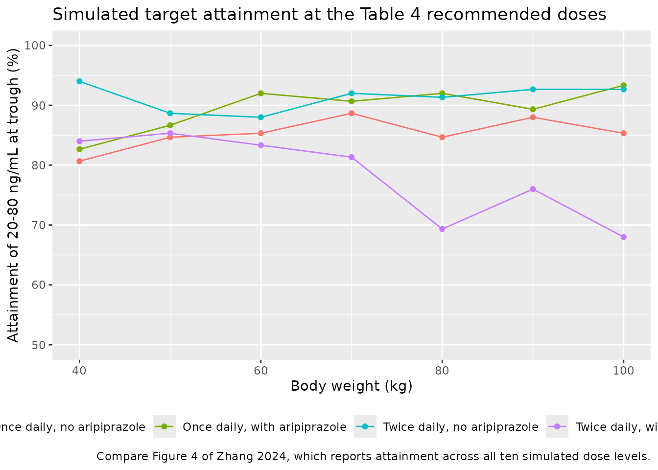
# GATED: the once-daily arms, where the trough criterion reproduces Table 4.
# `gap_pts` is the non-overlap between the simulated and published attainment
# RANGES, so it is 0 whenever they intersect. The bound is generous relative to
# both Monte Carlo noise (SE ~ 2.5 points at 150 subjects per arm and 90%
# attainment) and the thread-count spread that rxSetSeed cannot remove. It is
# not a gate that cannot fail: the ungated "Twice daily, with aripiprazole" row
# scores 10.8 on the same metric, and a mis-transcribed clearance, dose or
# omega shifts attainment by 15-30 points.
once_daily <- pta_summary |> dplyr::filter(grepl("^Once daily", condition))
stopifnot(nrow(once_daily) == 2L, all(once_daily$gap_pts < 10))

# NOT GATED: the twice-daily arms are a documented deviation (see below).
# Recorded so the table stays honest rather than widened until it passes.
twice_daily <- pta_summary |> dplyr::filter(grepl("^Twice daily", condition))
stopifnot(nrow(twice_daily) == 2L)
The once-daily arms reproduce Table 4 to within a few percentage points. The twice-daily arms do not, and the reason is visible in the deterministic Figure 3 replication above rather than in the cohort. At 100 kg on 0.4 mg/kg/day with aripiprazole – a cell Table 4 credits with 99.5-99.9% attainment – the typical patient, carrying no between-subject variability at all, already has an average steady-state concentration of 76 ng/mL and a peak above the 80 ng/mL ceiling. Adding 32% CV on clearance around that centre can only lower attainment further, so no criterion recovers 99.5%. This is a property of the published attainment table, not of the structural model, which matches Table 3 exactly (see the NCA section).
Assumptions and deviations
-
omega_CL/F= 0.316 is read as a standard deviation, not a variance. Two independent lines of evidence support this. (1) Notation: Methods Equation (1) definesetaas having “variance omega^2 (omega^2)”, and the Table 3 row is labelledomega_CL/F, notomega^2; the same holds forsigma_1andsigma_2against Equation (2)’s “variance sigma^2”. (2) The paper’s own simulation output: reading 0.316 as a variance gives an inter-individual SD of 0.562 on the log scale, and target attainment then falls 20-30 percentage points below every cell of Table 4 under any criterion (trough, interval average, or whole profile), whereas the SD reading reproduces the once-daily cells to within a few points. The model therefore encodesetalcl ~ 0.316^2, i.e. 32.4% CV.propSd = 0.288andaddSd = 3.701 ng/mLare read on the same convention. - The paper’s target-attainment criterion is not stated. Methods, Simulation says only “The evaluation criterion was the probability for achieving target concentration” against 20-80 ng/mL. This vignette uses the steady-state trough. Under that criterion the once-daily recommendations reproduce; the twice-daily ones do not, and no alternative criterion tested (interval average, entire profile within the band, trough only) reproduces all four conditions simultaneously. The twice-daily rows are reported as a known deviation and excluded from the gate rather than having the tolerance widened until they pass.
- Doses and sampling times are constructed, not observed. The source concentrations come from a routine TDM database and the paper reports no administered doses, dose ranges or sampling schedule, so no observed-data replication is possible. Every regimen simulated here is either a Table 4 recommendation or a single 10 mg dose chosen to exercise the NCA identities.
- Steady state is reached by simulation, not assumed. A 480 h run-in is used throughout, which is more than 13 half-lives even for the slowest arm (aripiprazole co-administration, t1/2 = 35.3 h).
-
kaand both allometric exponents arefixed().ka = 0.861 1/his quoted by Zhang 2024 from Sun 2021 (their reference 29) and printed as “0.861 (fixed)” in Table 3 with no SE and no bootstrap row. The exponents 0.75 and 1 are asserted in Methods Equation (3) from Anderson & Holford (2008) and appear in no results table. None of the three is an estimate of this study. -
No IIV on V/F or ka, and no correlation structure.
Table 3 reports a single
omegarow. This is encoded faithfully as a single-eta model rather than adding variability the paper did not report. - Body weight is time-fixed. The paper reports one weight per patient from a retrospective medical log.
-
CONMED_ARIPIPRAZOLEis a new canonical covariate column, registered ininst/references/covariate-columns.mdin the same change as this model. It encodes the paper’sARIvariable with the same 0/1 orientation. - Supplementary Table S1 was not available when this model was built. It contains the per-drug hypothesis tests (objective-function changes) for the 30 screened concomitant medications. It holds no model parameter values – the final model is fully specified by Equations (6) and (7) and Table 3 – so its absence does not affect the extraction. The stepwise result it documents (only aripiprazole retained) is stated in the main text.
-
Four exposed patients. The
-0.392aripiprazole coefficient rests on 4 of 65 patients (Table 2), and its bootstrap 95% interval is correspondingly wide ([-0.535, -0.194]). The point estimate is used here as published, but any downstream use should carry that interval. -
Screened-but-unretained covariates. Age, sex, and
the clinical-chemistry panel of Table 1 are recorded in the model’s
covariatesDataExcludedmetadata. Globulin, total protein, mean corpuscular hemoglobin and mean corpuscular hemoglobin concentration were also screened but have no canonical covariate-column entry, so they are recorded inpopulation$notesinstead.