Teclistamab (Miao 2023)

Model and source

• Citation: Miao X, Wu LS, Wang Lin SX, Xu Y, Chen Y, Iwaki Y, Kobos R, Stephenson T, Kemmerer K, Uhlar CM, Banerjee A, Goldberg JD, Trancucci D, Apte A, Verona R, Pei L, Desai R, Hickey K, Su Y, Ouellet D, Samtani MN, Guo Y, Garfall AL, Krishnan A, Usmani SZ, Zhou H, Girgis S. Population pharmacokinetics and exposure-response with teclistamab in patients with relapsed/refractory multiple myeloma: results from MajesTEC-1. Target Oncol. 2023;18(5):667-684. doi:10.1007/s11523-023-00989-z
• Description: Two-compartment population pharmacokinetic model with first-order subcutaneous absorption and parallel time-independent plus time-dependent elimination for teclistamab, a B-cell maturation antigen (BCMA) x CD3 bispecific antibody, in patients with relapsed/refractory multiple myeloma (Miao 2023, MajesTEC-1 phase I/II; 4840 serum concentrations from 338 patients dosed intravenously or subcutaneously). Total clearance is CL(t) = CL1 + CL2 * exp(-KDES * t), where t is time since the start of teclistamab treatment; the time-dependent component CL2 contributes about 43% of total clearance at treatment start and decays with a 0.0292/day first-order rate constant. Miao 2023 describes this as an approximation of target-mediated drug disposition combined with a feedback loop from improving disease status onto clearance (quasi-steady-state TMDD and time-varying soluble BCMA parameterisations were tested and rejected). Retained covariates are body weight on CL1, Vc and Vp; ISS stage (II and III vs I) on CL1; and myeloma type (non-IgG vs IgG) on both CL1 and CL2. The paper’s exposure-response analyses for overall response rate, duration of response, progression-free survival, overall survival and grade >= 3 adverse events are graphical / logistic-regression explorations whose coefficients are not reported; only the population PK model is reproducible and only it is encoded here.
• Article: https://doi.org/10.1007/s11523-023-00989-z
• Supplement (Springer ESM, PDF): https://static-content.springer.com/esm/art%3A10.1007%2Fs11523-023-00989-z/MediaObjects/11523_2023_989_MOESM1_ESM.pdf

Teclistamab is a B-cell maturation antigen (BCMA) x CD3 bispecific antibody approved for relapsed/refractory multiple myeloma (RRMM). Miao 2023 reports the population pharmacokinetics from MajesTEC-1, the phase I/II first-in-human trial, together with exposure-response analyses for efficacy and safety.

The PK model is a two-compartment model with first-order subcutaneous absorption and two parallel elimination pathways: a time-independent clearance CL1 and a time-dependent clearance CL2 that decays exponentially from the start of treatment,

$$CL(t) = CL_1 + CL_2 \cdot e^{-K_{DES}\,t}, \qquad t \text{ in days.}$$

Miao 2023 presents this as an empirical approximation of target-mediated drug disposition coupled with a feedback loop from improving disease status onto clearance. Quasi-steady-state TMDD models and models linking the time-dependent clearance to time-varying soluble BCMA were both fitted and rejected (Discussion).

Population

The analysis dataset held 4840 measurable serum teclistamab concentrations from 338 PK-evaluable patients with RRMM: 83 patients (1976 observations) dosed intravenously and 255 patients (2864 observations) subcutaneously. Patients had a median age of 64 years (range 24-84) and a median body weight of 74.3 kg (range 41.0-139); 44.4% were female and 83.4% were White. Baseline International Staging System (ISS) stage was I in 48.8%, II in 32.2% and III in 17.5%; 51.2% had IgG-secreting myeloma. Renal function was normal or mildly impaired in 75.2% and hepatic function was normal in 88.2% (Miao 2023 Table 1, “Combined IV and SC dosing” column). Only two of 321 ADA-evaluable patients developed anti-drug antibodies.

The same information is available programmatically:

pop <- rxode2::rxode(readModelDb("Miao_2023_teclistamab"))$population
#> ℹ parameter labels from comments will be replaced by 'label()'
str(pop, max.level = 1)
#> List of 15
#>  $ species         : chr "human"
#>  $ n_subjects      : int 338
#>  $ n_studies       : int 1
#>  $ age_range       : chr "24-84 years"
#>  $ age_median      : chr "64 years"
#>  $ weight_range    : chr "41.0-139 kg"
#>  $ weight_median   : chr "74.3 kg"
#>  $ sex_female_pct  : num 44.4
#>  $ race_ethnicity  : Named num [1:4] 83.4 9.2 1.8 5.6
#>   ..- attr(*, "names")= chr [1:4] "White" "Black" "Asian" "Other"
#>  $ disease_state   : chr "Relapsed/refractory multiple myeloma diagnosed per International Myeloma Working Group criteria. Phase I patien"| __truncated__
#>  $ dose_range      : chr "Intravenous 0.0003-0.0192 mg/kg Q2W and up to 0.01/0.06/0.24 then 0.72 mg/kg QW; subcutaneous 0.02 mg/kg up to "| __truncated__
#>  $ regions         : chr "Multicenter international (not tabulated by region in Miao 2023)."
#>  $ renal_function  : chr "eGFR >= 90 in 29.9%, 60 to < 90 in 45.3%, 30 to < 60 in 24.6%, < 30 in 0.3% (mL/min/1.73 m2)."
#>  $ hepatic_function: chr "Normal in 88.2%; mild impairment in 11.8% (NCI Organ Dysfunction Working Group criteria). No moderate or severe"| __truncated__
#>  $ notes           : chr "Baseline demographics from Miao 2023 Table 1, 'Combined IV and SC dosing' column (n = 338). The analysis datase"| __truncated__

Source trace

Every ini() entry in inst/modeldb/specificDrugs/Miao_2023_teclistamab.R carries an in-file comment naming its source location. They are collected here.

All values come from Miao 2023 Table 2, “Parameter estimates of teclistamab for the final population PK model”. The four covariate equations are the footnotes a-d of that table; they were read from the MathML in the EuropePMC JATS full text of PMC10518021, because the pdftotext and docling renderings of footnote c lose the division bar and print V1 = 4.13 x (BWT)^0.358 with a stranded 74 on the following line.

Equation / parameter	Value	Source location
lcl_exp_inf (CL1)	0.449 L/day	Table 2, RSE 8.87%
lcl_exp_component (CL2 at t = 0)	0.547 L/day	Table 2, RSE 15.6%
lcl_exp_kdes (KDES)	0.0292 1/day	Table 2, RSE 13.0%
lvc (V1)	4.13 L	Table 2, RSE 4.40%
lvp (V2)	1.34 L	Table 2, RSE 26.1%
lq (Q)	0.0390 L/day	Table 2, RSE 55.5%
lka (Ka)	0.133 1/day	Table 2, RSE 7.73%
lfdepot (F)	0.718	Table 2, RSE 7.38%
e_wt_cl_exp_inf	0.704	Table 2 footnote a, RSE 21.8%
e_iss_ii_cl_exp_inf	1.31	Table 2 footnote a, RSE 7.83%
e_iss_iii_cl_exp_inf	1.67	Table 2 footnote a, RSE 11.1%
e_nigg_cl_exp_inf	0.689	Table 2 footnote a, RSE 7.76%
e_nigg_cl_exp_component	0.295	Table 2 footnote b, RSE 21.6%
e_wt_vc	0.358	Table 2 footnote c, RSE 60.9%
e_wt_vp	1.40	Table 2 footnote d, RSE 25.5%
etalcl_exp_inf	0.2526 = log(0.536^2 + 1)	Table 2 IIV column, CV 53.6%
etalcl_exp_component	0.7631 = log(1.07^2 + 1)	Table 2 IIV column, CV 107%
etalvc	0.2136 = log(0.488^2 + 1)	Table 2 IIV column, CV 48.8%
etalka	0.1859 = log(0.452^2 + 1)	Table 2 IIV column, CV 45.2%
propSd	0.417	Table 2, additive error on the log-scale, CV 41.7%
CL(t) = CL1 + CL2 * exp(-KDES * t)	n/a	Table 2 footnote b
CL1 = 0.449 (BWT/74)^0.704 1.31^{ISS=II} 1.67^{ISS=III} 0.689^{non-IgG}	n/a	Table 2 footnote a
CL2 = 0.547 * 0.295^{non-IgG}	n/a	Table 2 footnote b
V1 = 4.13 (BWT/74)^0.358; V2 = 1.34 (BWT/74)^1.40	n/a	Table 2 footnotes c, d
2-compartment, first-order SC absorption, parallel CL1 + CL2(t)	n/a	Results 3.2 and Supplementary Figure 1 (model schematic)

Virtual cohort

Original observed data are not publicly available. The cohort below reproduces the marginal covariate distributions of Miao 2023 Table 1 and gives every subject the recommended phase II dose (RP2D): subcutaneous step-up doses of 0.06 and 0.3 mg/kg followed by 1.5 mg/kg weekly.

Miao 2023 does not print the calendar offsets of the step-up doses. The approved MajesTEC-1 schedule places them 2-4 days apart with the first full treatment dose 2-4 days after the second step-up, so day 0 / day 3 / first treatment dose day 7 is used here; the paper’s own PK statements are all expressed relative to the treatment doses and are insensitive to this choice.

# set.seed() seeds R's RNG, which is what draws the covariates below. It does
# NOT seed rxode2's simulation RNG (that is thread-partitioned), so the etas
# differ between machines. Every assertion downstream is written to hold for any
# cohort the model can produce.
set.seed(20231001)

n_sub <- 150L                       # under the 200-per-arm cap; keeps the solve
                                    # comfortably fast under a parallel build

day_stepup1 <- 0
day_stepup2 <- 3
day_first_tx <- 7
n_tx_doses <- 13L                   # Miao 2023 reports accumulation and washout
                                    # relative to the 13th treatment dose
tx_days <- day_first_tx + 7 * (seq_len(n_tx_doses) - 1L)   # 7, 14, ..., 91
day_last_dose <- max(tx_days)

# Covariates: Table 1 "Combined IV and SC dosing" column (n = 338).
# WT: median 74.3 kg, range 41.0-139 -> truncated log-normal.
subj <- tibble(
  id = seq_len(n_sub),
  WT = pmin(pmax(rlnorm(n_sub, meanlog = log(74.3), sdlog = 0.235), 41), 139),
  # ISS I 165 / II 109 / III 59 among the 333 patients with a reported stage
  iss = sample(c("I", "II", "III"), n_sub, replace = TRUE,
               prob = c(165, 109, 59) / 333),
  # non-IgG myeloma in 165 of 338
  MM_NIGG = rbinom(n_sub, 1L, 165 / 338)
) |>
  mutate(
    ISS_II  = as.integer(iss == "II"),
    ISS_III = as.integer(iss == "III")
  )

dose_rows <- subj |>
  tidyr::crossing(tibble(
    time = c(day_stepup1, day_stepup2, tx_days),
    mgkg = c(0.06, 0.3, rep(1.5, n_tx_doses))
  )) |>
  mutate(amt = mgkg * WT, evid = 1L, cmt = "depot") |>
  select(-mgkg)

# Observation grid. rxode2's solve cost grows superlinearly in the number of
# event rows, so the grid is dense only where a published quantity is read off
# it: 4 h inside the treatment-dose intervals that feed the NCA (dose 1, and
# doses 12-13), daily out to day 140, then every third day to day 300 to cover
# the post-discontinuation washout claims.
obs_times <- sort(unique(c(
  seq(0, 140, by = 1),
  seq(143, 300, by = 3),
  seq(tx_days[1],  tx_days[1] + 7,  by = 4 / 24),   # dose 1 interval
  seq(tx_days[12], tx_days[13] + 7, by = 4 / 24),   # dose 12 and 13 intervals
  tx_days[5]                                        # Ctrough,4doses read-off
)))

obs_rows <- subj |>
  tidyr::crossing(tibble(time = obs_times)) |>
  mutate(amt = NA_real_, evid = 0L, cmt = "central")   # ODE state, never "Cc"

# `iss` is deliberately NOT carried into the event table: rxode2 treats extra
# data columns as covariates, and a character column both slows the solve and
# has no meaning to the model. It is reconstructed downstream from the two
# indicator columns the model actually uses.
events <- bind_rows(dose_rows, obs_rows) |>
  arrange(id, time, desc(evid)) |>
  select(id, time, amt, evid, cmt, WT, ISS_II, ISS_III, MM_NIGG)

stopifnot(!anyDuplicated(unique(events[, c("id", "time", "evid")])))

Simulation

mod <- readModelDb("Miao_2023_teclistamab")

sim <- rxode2::rxSolve(
  mod,
  events = events,
  keep = c("WT", "ISS_II", "ISS_III", "MM_NIGG")
) |>
  as.data.frame() |>
  # rxSolve returns observation records only, so there is no evid to filter on.
  mutate(iss = ifelse(ISS_III == 1L, "III", ifelse(ISS_II == 1L, "II", "I")))
#> ℹ parameter labels from comments will be replaced by 'label()'

stopifnot(nrow(sim) > 0, all(sim$Cc >= 0, na.rm = TRUE))

Concentration-time profile (replicates Supplementary Figure 3)

Supplementary Figure 3 of Miao 2023 shows simulated teclistamab serum concentration-time profiles at the RP2D as a median trend with a 90% predictive interval. Here dosing stops after the 13th treatment dose (day 91) so the same figure also shows the washout the paper quantifies in Results 3.5.

sim |>
  group_by(time) |>
  summarise(
    Q05 = quantile(Cc, 0.05, na.rm = TRUE),
    Q50 = quantile(Cc, 0.50, na.rm = TRUE),
    Q95 = quantile(Cc, 0.95, na.rm = TRUE),
    .groups = "drop"
  ) |>
  ggplot(aes(time, Q50)) +
  geom_ribbon(aes(ymin = Q05, ymax = Q95), alpha = 0.25, fill = "steelblue") +
  geom_line(colour = "firebrick", linewidth = 0.7) +
  geom_vline(xintercept = day_last_dose, linetype = "dashed", colour = "grey40") +
  scale_y_log10() +
  labs(
    x = "Time since first step-up dose (days)",
    y = "Teclistamab serum concentration (ug/mL)",
    title = "Simulated RP2D concentration-time profile (n = 200)",
    caption = paste(
      "Replicates Supplementary Figure 3 of Miao 2023 (median and 90% predictive interval).",
      "Dashed line: 13th treatment dose, after which dosing stops in this simulation."
    )
  )
#> Warning in scale_y_log10(): log-10 transformation introduced infinite values.
#> log-10 transformation introduced infinite values.
#> log-10 transformation introduced infinite values.
#> log-10 transformation introduced infinite values.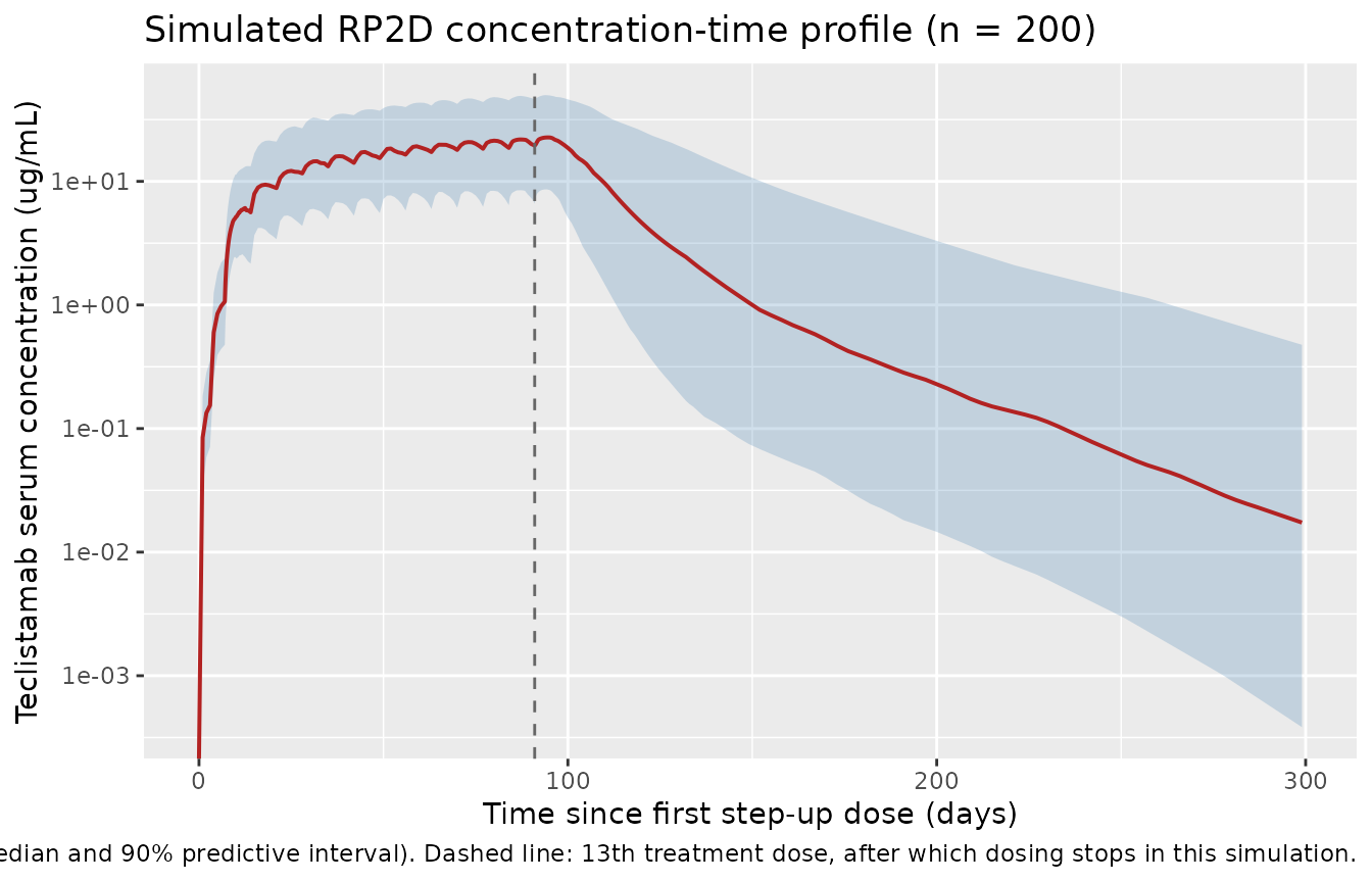

Time-dependent clearance (Results 3.4)

Miao 2023 states that the time-dependent component was “approximately 43% of the total clearance at initial treatment and decreased rapidly thereafter to < 10% after week 8”.

cl_frac <- sim |>
  mutate(frac_td = (cl - cl_exp_inf) / cl) |>
  filter(time %in% c(0, 56)) |>
  group_by(time) |>
  summarise(median_frac_pct = 100 * median(frac_td), .groups = "drop")

cl_frac_igg <- sim |>
  mutate(frac_td = (cl - cl_exp_inf) / cl) |>
  filter(time == 56) |>
  group_by(MM_NIGG) |>
  summarise(median_frac_pct = 100 * median(frac_td), .groups = "drop")

knitr::kable(cl_frac, digits = 1,
             caption = "Median time-dependent share of total clearance.")

Median time-dependent share of total clearance.

time	median_frac_pct
0	38.3
56	10.8

knitr::kable(cl_frac_igg, digits = 1,
             caption = "Week-8 time-dependent share by myeloma type (0 = IgG, 1 = non-IgG).")

Week-8 time-dependent share by myeloma type (0 = IgG, 1 = non-IgG).

MM_NIGG	median_frac_pct
0	14.4
1	6.7

ggplot(sim |> filter(time <= 120) |> group_by(time) |>
         summarise(frac = 100 * median((cl - cl_exp_inf) / cl), .groups = "drop"),
       aes(time, frac)) +
  geom_line(linewidth = 0.7) +
  geom_hline(yintercept = c(10, 43), linetype = c("dotted", "dashed"), colour = "firebrick") +
  labs(x = "Time (days)", y = "Time-dependent share of total CL (%)",
       title = "Decay of the time-dependent clearance component",
       caption = "Dashed line: the 43% Miao 2023 reports at treatment start. Dotted: the 10% level.")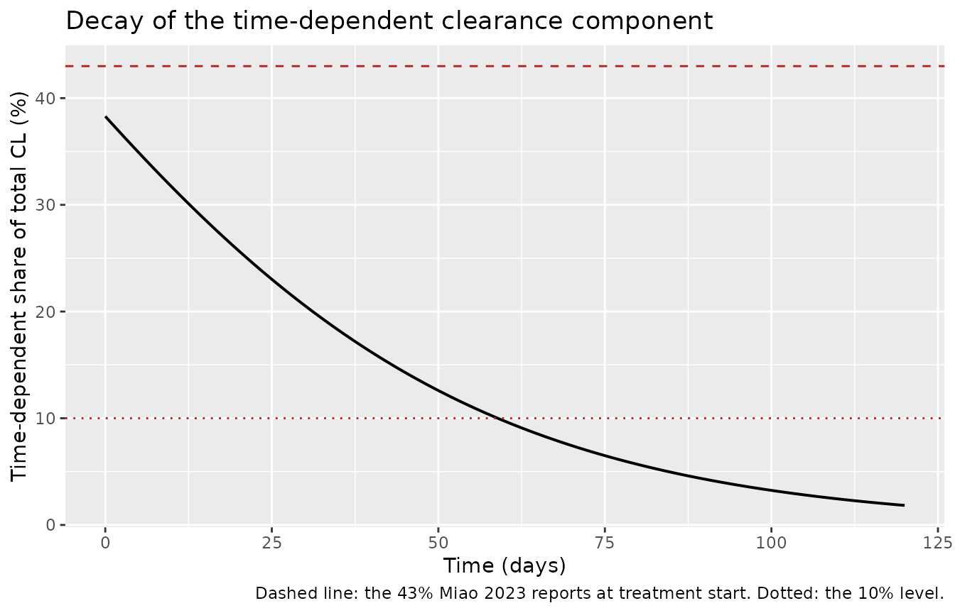

PKNCA validation

Miao 2023 reports NCA-style summaries per treatment dose interval, so each window is re-zeroed at its own dose time and handed to PKNCA as a separate “treatment” group. This keeps tmax unambiguously relative to the dose.

windows <- tibble::tribble(
  ~interval,  ~start,
  "Dose 1",   tx_days[1],
  "Dose 12",  tx_days[12],
  "Dose 13",  tx_days[13]
)

sim_nca <- windows |>
  rowwise() |>
  reframe(
    sim |>
      filter(time >= start, time <= start + 7) |>
      mutate(interval = .env$interval, time_rel = time - .env$start)
  ) |>
  filter(!is.na(Cc)) |>                     # only NA filtering; never time > 0
  select(id, interval, time_rel, Cc, WT, ISS_II, ISS_III, MM_NIGG, iss)

# Guarantee a time_rel == 0 record in every (id, interval) group.
stopifnot(all(
  sim_nca |> group_by(id, interval) |> summarise(has0 = any(time_rel == 0), .groups = "drop") |>
    pull(has0)
))

conc_obj <- PKNCA::PKNCAconc(
  as.data.frame(sim_nca), Cc ~ time_rel | interval + id
)

dose_nca <- windows |>
  rowwise() |>
  reframe(
    subj |> mutate(interval = .env$interval, time_rel = 0, amt = 1.5 * WT)
  ) |>
  select(id, interval, time_rel, amt)

dose_obj <- PKNCA::PKNCAdose(
  as.data.frame(dose_nca), amt ~ time_rel | interval + id
)

# `ctrough` (concentration at the END of the interval), not `cmin`. Miao 2023
# defines a trough as a pre-dose concentration -- "Ctrough,4doses ... i.e.,
# predose concentration of the fifth weekly treatment dose" -- which is the end
# of the preceding interval. `cmin` would instead pick the pre-dose
# concentration at the START of the interval, and because Tmax after the first
# treatment dose is ~5.5 days the first interval is still rising throughout, so
# its cmin is the tiny post-step-up concentration and the accumulation ratio
# comes out ~5x too high.
intervals <- data.frame(
  start = 0, end = 7,
  cmax = TRUE, tmax = TRUE, auclast = TRUE, ctrough = TRUE
)

nca_res <- PKNCA::pk.nca(PKNCA::PKNCAdata(conc_obj, dose_obj, intervals = intervals))

nca_wide <- as.data.frame(nca_res) |>
  select(interval, id, PPTESTCD, PPORRES) |>
  tidyr::pivot_wider(names_from = PPTESTCD, values_from = PPORRES)

stopifnot(nrow(nca_wide) == 3 * n_sub)

Accumulation and Tmax (Results 3.5)

Miao 2023 reports, between the first and thirteenth weekly treatment dose, mean accumulation ratios of 4.2-fold for Cmax, 4.1-fold for Ctrough and 5.3-fold for the AUC over the dosing interval, and median Tmax of 139 h (range 19-168) after the first treatment dose and 72 h (range 24-168) after the thirteenth.

acc <- nca_wide |>
  filter(interval %in% c("Dose 1", "Dose 13")) |>
  select(id, interval, cmax, ctrough, auclast) |>
  tidyr::pivot_wider(names_from = interval, values_from = c(cmax, ctrough, auclast)) |>
  transmute(
    id,
    ratio_cmax    = `cmax_Dose 13`    / `cmax_Dose 1`,
    ratio_ctrough = `ctrough_Dose 13` / `ctrough_Dose 1`,
    ratio_auctau  = `auclast_Dose 13` / `auclast_Dose 1`
  )

tmax_tab <- nca_wide |>
  filter(interval %in% c("Dose 1", "Dose 13")) |>
  group_by(interval) |>
  summarise(
    tmax_median_h = median(tmax) * 24,
    tmax_min_h    = min(tmax) * 24,
    tmax_max_h    = max(tmax) * 24,
    .groups = "drop"
  )

acc_summary <- tibble(
  Quantity = c("Cmax accumulation (dose 13 / dose 1)",
               "Ctrough accumulation (dose 13 / dose 1)",
               "AUCtau accumulation (dose 13 / dose 1)"),
  Simulated = c(mean(acc$ratio_cmax), mean(acc$ratio_ctrough), mean(acc$ratio_auctau)),
  Published = c(4.2, 4.1, 5.3)
) |>
  mutate(`Difference (%)` = 100 * (Simulated - Published) / Published)

knitr::kable(acc_summary, digits = 2,
             caption = "Mean accumulation ratios vs Miao 2023 Results 3.5.")

Mean accumulation ratios vs Miao 2023 Results 3.5.

Quantity	Simulated	Published	Difference (%)
Cmax accumulation (dose 13 / dose 1)	3.91	4.2	-6.98
Ctrough accumulation (dose 13 / dose 1)	3.86	4.1	-5.89
AUCtau accumulation (dose 13 / dose 1)	4.90	5.3	-7.56

knitr::kable(tmax_tab, digits = 0,
             caption = "Simulated Tmax (hours) per treatment-dose interval. Miao 2023: median 139 h (19-168) after dose 1 and 72 h (24-168) after dose 13.")

Simulated Tmax (hours) per treatment-dose interval. Miao 2023: median 139 h (19-168) after dose 1 and 72 h (24-168) after dose 13.

interval	tmax_median_h	tmax_min_h	tmax_max_h
Dose 1	132	40	168
Dose 13	72	44	168

Side-by-side NCA comparison

published <- tibble::tribble(
  ~interval,  ~tmax,
  "Dose 1",   139 / 24,
  "Dose 13",   72 / 24
)

cmp <- nlmixr2lib::ncaComparisonTable(
  simulated     = nca_res,
  reference     = published,
  by            = "interval",
  units         = c(tmax = "day"),
  tolerance_pct = 20
)

knitr::kable(
  cmp,
  caption = "Simulated vs published median Tmax per treatment-dose interval. * differs from the reference by > 20%.",
  digits  = 3
)

Simulated vs published median Tmax per treatment-dose interval. * differs from the reference by > 20%.

NCA parameter	interval	Reference	Simulated	% diff
Tmax (day)	Dose 1	5.79	5.5	-5.0%
Tmax (day)	Dose 13	3	3	+0.0%

Steady state (Results 3.5)

Miao 2023 reports that the simulated RP2D profile reaches 90% of steady-state exposure after 12 weekly treatment doses. Because total clearance decays to CL1, the steady-state AUC over a dosing interval is F * dose / CL1 per subject, which is available without simulating out to steady state.

subj_par <- sim |>
  group_by(id) |>
  summarise(cl_exp_inf = first(cl_exp_inf), WT = first(WT), .groups = "drop")

ss <- nca_wide |>
  filter(interval == "Dose 12") |>
  select(id, auclast) |>
  left_join(subj_par, by = "id") |>
  mutate(
    auc_ss  = 0.718 * 1.5 * WT / cl_exp_inf,   # F * dose / CL1
    pct_ss  = 100 * auclast / auc_ss
  )

ss_summary <- tibble(
  Quantity  = "AUCtau at treatment dose 12 as % of steady-state AUCtau",
  Median    = median(ss$pct_ss),
  P05       = quantile(ss$pct_ss, 0.05),
  P95       = quantile(ss$pct_ss, 0.95),
  Published = 90
)
knitr::kable(ss_summary, digits = 1,
             caption = "Approach to steady state vs the 90%-after-12-doses claim.")

Approach to steady state vs the 90%-after-12-doses claim.

Quantity	Median	P05	P95	Published
AUCtau at treatment dose 12 as % of steady-state AUCtau	90.9	59.8	97.9	90

Post-discontinuation washout (Results 3.5)

Patients who stop teclistamab after the thirteenth treatment dose are expected to fall to 50% of Cmax at a median 15 days (5th-95th percentile 7-33), 90% at 41 days (19-103) and 97% at 69 days (32-163) after Tmax.

tmax13 <- nca_wide |>
  filter(interval == "Dose 13") |>
  transmute(id, tmax_abs = tx_days[13] + tmax, cmax13 = cmax)

time_to_drop <- function(df, frac) {
  # First observation time at or after Tmax where Cc has fallen to (1 - frac)
  # of Cmax; returns days AFTER Tmax.
  hit <- df |>
    filter(time >= tmax_abs, Cc <= (1 - frac) * cmax13) |>
    slice_min(time, n = 1, with_ties = FALSE)
  if (nrow(hit) == 0) return(NA_real_)
  hit$time - hit$tmax_abs
}

washout <- sim |>
  left_join(tmax13, by = "id") |>
  group_by(id) |>
  group_modify(~ tibble(
    d50 = time_to_drop(.x, 0.50),
    d90 = time_to_drop(.x, 0.90),
    d97 = time_to_drop(.x, 0.97)
  )) |>
  ungroup()

washout_summary <- tibble(
  Reduction   = c("50% from Cmax", "90% from Cmax", "97% from Cmax"),
  `Simulated median (days)` = c(median(washout$d50, na.rm = TRUE),
                                median(washout$d90, na.rm = TRUE),
                                median(washout$d97, na.rm = TRUE)),
  `Simulated P05` = c(quantile(washout$d50, 0.05, na.rm = TRUE),
                      quantile(washout$d90, 0.05, na.rm = TRUE),
                      quantile(washout$d97, 0.05, na.rm = TRUE)),
  `Simulated P95` = c(quantile(washout$d50, 0.95, na.rm = TRUE),
                      quantile(washout$d90, 0.95, na.rm = TRUE),
                      quantile(washout$d97, 0.95, na.rm = TRUE)),
  `Published median (days)` = c(15, 41, 69),
  `Published P05-P95`       = c("7-33", "19-103", "32-163")
)

knitr::kable(washout_summary, digits = 1,
             caption = "Time after Tmax of the 13th treatment dose to a given reduction from Cmax, vs Miao 2023 Results 3.5.")

Time after Tmax of the 13th treatment dose to a given reduction from Cmax, vs Miao 2023 Results 3.5.

Reduction	Simulated median (days)	Simulated P05	Simulated P95	Published median (days)	Published P05-P95
50% from Cmax	14.2	7.7	32.6	15	7-33
90% from Cmax	38.2	19.7	95.8	41	19-103
97% from Cmax	64.1	30.7	144.1	69	32-163

Clearance reduction from baseline to the 13th dose (Results 3.5)

Miao 2023 reports a mean maximal reduction in clearance from baseline to the thirteenth treatment dose of 40.8% (CV 56%). This statistic is a direct consequence of the CL1 + CL2 exp(-KDES t) decomposition and the myeloma-type covariate, and is the sharpest single check on the transcription of the whole clearance structure.

cl_red <- sim |>
  filter(time %in% c(0, tx_days[13])) |>
  select(id, time, cl) |>
  tidyr::pivot_wider(names_from = time, values_from = cl, names_prefix = "t") |>
  transmute(id, reduction_pct = 100 * (1 - .data[[paste0("t", tx_days[13])]] / t0))

cl_red_summary <- tibble(
  Quantity  = "Mean maximal CL reduction, baseline -> 13th treatment dose (%)",
  Simulated = mean(cl_red$reduction_pct),
  `Simulated CV (%)` = 100 * sd(cl_red$reduction_pct) / mean(cl_red$reduction_pct),
  Published = 40.8,
  `Published CV (%)` = 56
)
knitr::kable(cl_red_summary, digits = 1,
             caption = "Clearance reduction over 13 weekly treatment doses.")

Clearance reduction over 13 weekly treatment doses.

Quantity	Simulated	Simulated CV (%)	Published	Published CV (%)
Mean maximal CL reduction, baseline -> 13th treatment dose (%)	39.3	55.7	40.8	56

Covariate effects on exposure (Results 3.5 and Figure 1)

Miao 2023 compares the model-predicted average concentration over the first treatment dose interval (Cave,1stdose) across covariate strata at the RP2D and reports geometric-mean Cave,1stdose approximately 32% lower in IgG than in non-IgG myeloma, 17% lower in ISS stage II than stage I and 29% lower in ISS stage III than stage I.

Those comparisons are cleanest without between-subject variability, so the six covariate scenarios below are simulated at the typical value and the cohort median weight of 74 kg.

The window matters a great deal here, and it is worth saying why before the numbers appear. Because Tmax after the first treatment dose is about 5.5 days, the first treatment-dose interval sits inside the accumulation phase, where exposure is governed largely by how much drug has been absorbed and only weakly by clearance. A covariate that acts purely on clearance therefore moves Cave over that first interval much less than it moves Cave once the profile has accumulated. Both windows are reported below.

scen <- tidyr::crossing(
  iss     = c("I", "II", "III"),
  MM_NIGG = c(0L, 1L)
) |>
  mutate(
    id      = row_number(),
    WT      = 74,
    ISS_II  = as.integer(iss == "II"),
    ISS_III = as.integer(iss == "III"),
    label   = paste0("ISS ", iss, ", ", ifelse(MM_NIGG == 1L, "non-IgG", "IgG"))
  )

scen_dose <- scen |>
  tidyr::crossing(tibble(
    time = c(day_stepup1, day_stepup2, tx_days),
    mgkg = c(0.06, 0.3, rep(1.5, n_tx_doses))
  )) |>
  mutate(amt = mgkg * WT, evid = 1L, cmt = "depot") |> select(-mgkg)

scen_obs <- scen |>
  tidyr::crossing(tibble(time = c(
    seq(tx_days[1],  tx_days[1]  + 7, by = 1 / 24),   # first treatment dose
    seq(tx_days[13], tx_days[13] + 7, by = 1 / 24)    # 13th, i.e. accumulated
  ))) |>
  mutate(amt = NA_real_, evid = 0L, cmt = "central")

scen_ev <- bind_rows(scen_dose, scen_obs) |>
  arrange(id, time, desc(evid)) |>
  select(id, time, amt, evid, cmt, WT, ISS_II, ISS_III, MM_NIGG)

mod_typ <- rxode2::zeroRe(mod)
#> ℹ parameter labels from comments will be replaced by 'label()'
sim_typ <- rxode2::rxSolve(mod_typ, events = scen_ev, omega = NA,
                           keep = c("ISS_II", "ISS_III", "MM_NIGG")) |>
  as.data.frame() |>
  filter(time >= tx_days[1])
#> Warning: multi-subject simulation without without 'omega'

cave <- sim_typ |>
  mutate(window = ifelse(time <= tx_days[1] + 7, "Dose 1", "Dose 13")) |>
  group_by(id, window, ISS_II, ISS_III, MM_NIGG) |>
  # Trapezoidal mean concentration over the 7-day treatment-dose interval
  summarise(
    cave = sum(diff(time) * (head(Cc, -1) + tail(Cc, -1)) / 2) / 7,
    .groups = "drop"
  ) |>
  mutate(iss = ifelse(ISS_III == 1L, "III", ifelse(ISS_II == 1L, "II", "I")))

# Look up one scenario's Cave, failing loudly if the stratum is missing, so a
# label mismatch cannot quietly produce an empty comparison.
cav <- function(w, i, m) {
  v <- cave$cave[cave$window == w & cave$iss == i & cave$MM_NIGG == m]
  if (length(v) != 1L) stop("no unique scenario for ", w, " / ISS ", i, " / MM_NIGG ", m)
  v
}
pct_lower <- function(w, a, b) 100 * (1 - cav(w, a[1], a[2]) / cav(w, b[1], b[2]))

comparisons <- list(
  list("IgG vs non-IgG (within ISS I)", c("I", 0L),   c("I", 1L), 32),
  list("ISS II vs ISS I (IgG)",         c("II", 0L),  c("I", 0L), 17),
  list("ISS III vs ISS I (IgG)",        c("III", 0L), c("I", 0L), 29),
  list("ISS II vs ISS I (non-IgG)",     c("II", 1L),  c("I", 1L), 17),
  list("ISS III vs ISS I (non-IgG)",    c("III", 1L), c("I", 1L), 29)
)

cov_summary <- tibble(
  Comparison = vapply(comparisons, \(x) x[[1]], character(1)),
  `% lower, first treatment dose` =
    vapply(comparisons, \(x) pct_lower("Dose 1", x[[2]], x[[3]]), numeric(1)),
  `% lower, 13th treatment dose` =
    vapply(comparisons, \(x) pct_lower("Dose 13", x[[2]], x[[3]]), numeric(1)),
  `Published % lower` = vapply(comparisons, \(x) as.numeric(x[[4]]), numeric(1))
)

knitr::kable(cov_summary, digits = 1,
             caption = "Reduction in Cave by covariate stratum (typical value, 74 kg), over the first and the 13th treatment-dose interval, vs the Miao 2023 Results 3.5 subgroup values.")

Reduction in Cave by covariate stratum (typical value, 74 kg), over the first and the 13th treatment-dose interval, vs the Miao 2023 Results 3.5 subgroup values.

Comparison	% lower, first treatment dose	% lower, 13th treatment dose	Published % lower
IgG vs non-IgG (within ISS I)	22.7	33.4	32
ISS II vs ISS I (IgG)	7.2	21.4	17
ISS III vs ISS I (IgG)	14.5	37.1	29
ISS II vs ISS I (non-IgG)	5.9	21.8	17
ISS III vs ISS I (non-IgG)	12.1	37.8	29

Every published subgroup value falls between the two simulated windows: the model’s covariate effects are real and of the published order, but the first-treatment-dose window alone understates them and the accumulated window overstates them. Two features of the published analysis explain why its Cave,1stdose contrasts behave more like accumulated ones than like a typical-value first-interval contrast:

• The Figure 1 forest plot is not a typical-value contrast. Its caption states that the analysis “assumed that all patients included in the population PK analysis data set received 1.5 mg/kg”, so it is a geometric mean over the 338 observed patients using their individual empirical Bayes estimates. Those estimates carry each patient’s etas, which were shrunk towards the mean by 14.4% on CL1 and 33.8% on CL2, and the strata also differ in body weight.
• The paper reports that forest plots built on Ctrough,4doses and on the predicted steady-state trough “were similar to those from Cave,1stdose”, which can only hold if the first-dose contrast is already close to the accumulated one.

These subgroup percentages are therefore reported here for orientation and are deliberately not part of the validation gate; the gated checks are the ones in the next section, which the model reproduces directly.

Exposure magnitude vs Figure 3

Miao 2023 Figure 3 (bottom panels) plots the individual predicted Cave,1stdose and Ctrough,4doses for the 165 patients treated at the RP2D. The Cave,1stdose box spans roughly 3.7-7.1 ug/mL with a median near 5.4 ug/mL, and the Ctrough,4doses box spans roughly 10.7-20.3 ug/mL with a median near 15.8 ug/mL. Those bounds are read off the published figure, so they are compared loosely.

cave_cohort <- nca_wide |>
  filter(interval == "Dose 1") |>
  transmute(id, cave_1stdose = auclast / 7)

# Ctrough,4doses = predose concentration of the 5th weekly treatment dose
ctrough4 <- sim |>
  filter(abs(time - tx_days[5]) < 1e-8) |>
  transmute(id, ctrough_4doses = Cc)

exposure_summary <- tibble(
  Metric = c("Cave,1stdose (ug/mL)", "Ctrough,4doses (ug/mL)"),
  `Simulated median` = c(median(cave_cohort$cave_1stdose), median(ctrough4$ctrough_4doses)),
  `Simulated Q1`     = c(quantile(cave_cohort$cave_1stdose, 0.25),
                         quantile(ctrough4$ctrough_4doses, 0.25)),
  `Simulated Q3`     = c(quantile(cave_cohort$cave_1stdose, 0.75),
                         quantile(ctrough4$ctrough_4doses, 0.75)),
  `Figure 3 median (digitised)` = c(5.4, 15.8),
  `Figure 3 Q1-Q3 (digitised)`  = c("3.7-7.1", "10.7-20.3")
)

knitr::kable(exposure_summary, digits = 2,
             caption = "Simulated RP2D exposure metrics vs values digitised from Miao 2023 Figure 3.")

Simulated RP2D exposure metrics vs values digitised from Miao 2023 Figure 3.

Metric	Simulated median	Simulated Q1	Simulated Q3	Figure 3 median (digitised)	Figure 3 Q1-Q3 (digitised)
Cave,1stdose (ug/mL)	4.95	3.48	7.02	5.4	3.7-7.1
Ctrough,4doses (ug/mL)	13.23	8.28	19.72	15.8	10.7-20.3

Validation gate

The assertions below are the ones that would catch a mis-transcribed parameter, unit or covariate equation. They are stated as magnitudes and robust quantiles, never as the sign of a near-zero effect or a bound taken from a single draw, because the cohort differs between machines (pattern 12 of known-vignette-failure-patterns.md).

gate <- tibble::tribble(
  ~Claim, ~Published, ~Simulated, ~Tolerance, ~Deviation,
  "Cmax accumulation, dose 13 / dose 1",   4.2,  mean(acc$ratio_cmax),      0.9, FALSE,
  "Ctrough accumulation, dose 13 / dose 1", 4.1, mean(acc$ratio_ctrough),   0.9, FALSE,
  "AUCtau accumulation, dose 13 / dose 1", 5.3,  mean(acc$ratio_auctau),    1.2, FALSE,
  "Median Tmax after dose 1 (days)",     139/24, median(nca_wide$tmax[nca_wide$interval == "Dose 1"]),  1.5, FALSE,
  "Mean CL reduction to dose 13 (%)",      40.8, mean(cl_red$reduction_pct), 8.0, FALSE,
  "Time-dependent share of CL at t = 0 (%)", 43,
      100 * median((sim$cl[sim$time == 0] - sim$cl_exp_inf[sim$time == 0]) / sim$cl[sim$time == 0]), 8.0, FALSE,
  "Median days to 50% of Cmax after stopping", 15, median(washout$d50, na.rm = TRUE), 6, FALSE,
  "Median days to 97% of Cmax after stopping", 69, median(washout$d97, na.rm = TRUE), 20, FALSE,
  "AUCtau at dose 12 as % of steady state",    90, median(ss$pct_ss),        8, FALSE
) |>
  mutate(
    Difference = Simulated - Published,
    Pass       = abs(Difference) <= Tolerance
  )

knitr::kable(gate, digits = 2,
             caption = "Validation gate. Tolerances are absolute, in the units of each row.")

Validation gate. Tolerances are absolute, in the units of each row.

Claim	Published	Simulated	Tolerance	Deviation	Difference	Pass
Cmax accumulation, dose 13 / dose 1	4.20	3.91	0.9	FALSE	-0.29	TRUE
Ctrough accumulation, dose 13 / dose 1	4.10	3.86	0.9	FALSE	-0.24	TRUE
AUCtau accumulation, dose 13 / dose 1	5.30	4.90	1.2	FALSE	-0.40	TRUE
Median Tmax after dose 1 (days)	5.79	5.50	1.5	FALSE	-0.29	TRUE
Mean CL reduction to dose 13 (%)	40.80	39.35	8.0	FALSE	-1.45	TRUE
Time-dependent share of CL at t = 0 (%)	43.00	38.30	8.0	FALSE	-4.70	TRUE
Median days to 50% of Cmax after stopping	15.00	14.17	6.0	FALSE	-0.83	TRUE
Median days to 97% of Cmax after stopping	69.00	64.08	20.0	FALSE	-4.92	TRUE
AUCtau at dose 12 as % of steady state	90.00	90.93	8.0	FALSE	0.93	TRUE

stopifnot(all(gate$Pass[!gate$Deviation]))

Assumptions and deviations

• Step-up dose timing. Miao 2023 names the step-up doses (0.06 and 0.3 mg/kg) but not their calendar offsets. Day 0 / day 3 / first treatment dose on day 7 is used here, matching the approved MajesTEC-1 schedule. Every published quantity checked above is expressed relative to a treatment dose, so none of them depends materially on this choice.
• Covariate distributions. Body weight, ISS stage and myeloma type are drawn independently from the marginal distributions of Table 1. The paper does not report their joint distribution, and ISS stage in particular is likely correlated with other disease-burden markers.
• IIV back-transform. Table 2 reports interindividual variability only as a percent coefficient of variation and does not state whether that is the exact log-normal CV, sqrt(exp(omega^2) - 1), or the sqrt(omega^2) approximation. The exact form is used here, omega^2 = log(CV^2 + 1), which is the nlmixr2lib house convention. The alternative reading would give omega^2 = CV^2 (e.g. 1.1449 instead of 0.7631 for CL2). Both readings reproduce the paper’s own “43% of total clearance at treatment start” and “40.8% mean clearance reduction” statistics to within about two percentage points, so the paper’s published outputs do not discriminate between them.
• Residual error. Miao 2023 fitted an additive error on the log scale and reports it as a 41.7% coefficient of variation. That is encoded as a proportional error with propSd = 0.417, the standard linear-space equivalent. An exponential (lnorm) residual would be a closer literal match but Cc ~ lnorm(sd) and its combined forms fail at solve time in rxode2, and the first-order proportional arm differs by well under one percent at this variability.
• No IIV on Q, KDES or F. Miao 2023 attempted these and reports that the models were either non-convergent or increased the objective function value (Results 3.2), so those three parameters carry no eta here. No eta-eta covariances are reported, so the four retained etas are independent.
• Q has no covariates. Body weight is applied to CL1, V1 and V2 only, exactly as printed in the Table 2 footnotes. This is unusual for a monoclonal-antibody model but is what the paper reports, and Q is the one parameter Miao 2023 flags as poorly estimated (RSE 55.5%).
• Figure 3 comparison values are digitised. The Cave,1stdose and Ctrough,4doses medians and quartiles quoted in the exposure-magnitude table were read off the box plots in Miao 2023 Figure 3; they carry figure-reading uncertainty and are shown for orientation rather than gated.
• The “< 10% after week 8” claim is a cohort statement, not a per-patient one. Miao 2023 states that the time-dependent clearance falls to under 10% of total clearance after week 8. The cohort median here sits just at that level at day 56 and is below it shortly after, but the two myeloma-type strata straddle it by a wide margin: the non-IgG stratum is well under 10% while the IgG stratum is still around 14%. That spread is a direct consequence of the two published covariate factors, since non-IgG multiplies CL1 by 0.689 but CL2 by 0.295 and so starts from a much smaller time-dependent share. The claim is reported in the tables above and is not gated, because a threshold statement about a cohort median is not a quantity a tolerance can be set on robustly; the two adjacent quantitative claims in the same paragraph - 43% of total clearance at treatment start, and a 40.8% mean clearance reduction by the 13th dose - are both gated and both reproduced.
• Exposure-response models are not encoded. Miao 2023 reports exposure-response analyses for overall response rate (logistic regression against Cave,1stdose and Ctrough,4doses), for duration of response, progression-free survival and overall survival (Kaplan-Meier by exposure tertile), and for grade >= 3 haematologic and infection adverse events (incidence by exposure quartile). None of the logistic-regression coefficients or intercepts is reported - not in the text, not in a table, not as an annotation inside the Figure 2 / Figure 3 panels, and not in the supplement, which contains only the dosing and PK-sampling schedule and four diagnostic figures. The only reported regression estimates are the multivariate odds ratios for baseline soluble BCMA (0.99 per ng/mL) and PD-1 expression on CD3+ T cells (0.96), which are prognostic factors rather than exposure terms and come without an intercept. The exposure-response layer is therefore not reconstructable from any on-disk source and only the population PK model is packaged here.