Venetoclax and B-lymphocytes in healthy subjects (Dave 2019)
Source:vignettes/articles/Dave_2019_venetoclax.Rmd
Dave_2019_venetoclax.RmdModel and source
- Citation: Dave N, Gopalakrishnan S, Mensing S, Salem AH. Model-Informed Dosing of Venetoclax in Healthy Subjects: An Exposure-Response Analysis. Clin Transl Sci. 2019;12(6):625-632. doi:10.1111/cts.12665. Parameter estimates from Table 2; model code from the Supporting Information ‘PK Model code’ (CTS-12-625-s003.pdf) and ‘PD Model code’ (CTS-12-625-s002.pdf) NONMEM control streams. Lymphocyte model backbone: Friberg LE et al. J Clin Oncol 2002;20(24):4713-4721, doi:10.1200/JCO.2002.02.140.
- Description: Integrated population PK / semimechanistic PD model for venetoclax and circulating B-lymphocytes in healthy female subjects. PK: two-compartment model with first-order absorption, an absorption lag time under fed conditions only, and first-order elimination; relative bioavailability depends on food (fasting / low-fat reference / moderate-or-high-fat), azithromycin coadministration, Chinese ethnicity, rifampin coadministration and a fixed power function of dose, and rifampin also raises apparent clearance. PD: Friberg-type lymphocyte model (proliferating pool, three transit compartments, circulating B-lymphocytes) with a (baseline / circulating)^gamma feedback on proliferation and a linear venetoclax effect increasing the first-order loss of circulating B-lymphocytes. The individual observed pre-dose B-lymphocyte count is the PD baseline. Final IIV and residual-error magnitudes are not reported by the source, so every random effect and residual SD is fixed(0): the model reproduces typical-value predictions only.
- Article: https://doi.org/10.1111/cts.12665 (open access; PMC6853148)
- Supplement: NONMEM control streams “PK Model code” and “PD Model code” (Supporting Information, CTS-12-625-s003.pdf and CTS-12-625-s002.pdf)
Dave et al. pooled 10 healthy-volunteer clinical pharmacology studies to relate venetoclax exposure to the on-target decrease in circulating B-lymphocytes. A two-compartment population PK model was fit first. Its individual post hoc parameters then drove a semimechanistic Friberg-type lymphocyte model. In that model venetoclax concentration increases the first-order loss of circulating B-lymphocytes linearly. The paper uses the model to choose safe single and repeated doses for future studies in healthy volunteers.
The packaged model joins the two stages into one ODE system. The PK layer uses the population PK equations and Table 2 estimates, and the PD layer uses the PD control stream and Table 2 estimates.
Population
The analysis included 203 healthy female subjects (males were excluded because of a testicular-toxicity finding in 4-week dog studies), aged 21-65 years (median 40), with body mass index 18.6-30.1 kg/m^2. Twelve subjects were Chinese (Study I). Single oral venetoclax doses of 10-400 mg were given 1-4 times per subject, separated by washouts of at least 7 days. Doses were given either fasting or after a low-, moderate- or high-fat breakfast. The pooled studies included drug-drug interaction arms with ritonavir, digoxin, azithromycin, rifampin and warfarin (Table 1). B-lymphocytes were measured in 7 of the 10 studies, and only those studies entered the PD fit.
The same information is available programmatically via
readModelDb("Dave_2019_venetoclax")()$population.
Source trace
Every ini() value carries an in-file comment in
inst/modeldb/specificDrugs/Dave_2019_venetoclax.R. The
table collects them.
| Equation / parameter | Value | Source location |
|---|---|---|
lcl (CL/F) |
log(449) L/day | Table 2 ‘CL/F (L/day)’ |
lvc (V2/F) |
log(99) L | Table 2 ‘V2 (L)’ |
lq (Q/F) |
log(130) L/day | Table 2 ‘Q (L/day)’ |
lvp (V3/F) |
log(147) L | Table 2 ‘V3 (L)’ |
lka (KA) |
log(3.83) 1/day | Table 2 ‘KA (1/day)’ |
ltlag (ALAG, fed only) |
log(0.04) day | Table 2 ‘ALAG (day)’; PK code
IF(FOOD.GE.1) ALAG1 = THETA(8)
|
e_conmed_rifampicin_cl |
2.67 | Table 2 ‘Rifampin on CL’; PK code
CL = THETA(1)*THETA(15)
|
lfdepot |
fixed(log(1)) | Table 2 ‘Low fat on F1’ = 1; PK code TVF1=1,
TVFA=1
|
e_fasted_fdepot |
0.29 | Table 2 ‘Fasting on F1’ |
e_modhighfat_fdepot |
1.47 | Table 2 ‘Moderate/high-fat on F1’ |
e_conmed_azithromycin_fdepot |
0.65 | Table 2 ‘Azithromycin on F1’ |
e_race_chinese_fdepot |
1.53 | Table 2 ‘Chinese on F1’ |
e_conmed_rifampicin_fdepot |
4.91 | Table 2 ‘Rifampin on F1’ |
e_dose_fdepot |
fixed(-0.178) | Table 2 ‘Dose nonlinearity on F1’ (Fixed); PK code
(DOSE/400)**(THETA(14))
|
lthalf |
log(37.5) day | Table 2 ‘t 1/2 (days)’; PD code
DELTA = LOG(2)/THETA(1)
|
lktr (kin = ktr) |
log(0.1) 1/day | Table 2 ‘k in, proliferation (and transit maturation) rate’; PD code
KTR = KIN
|
lgamma |
log(0.1) | Table 2 ‘Feedback exponent’ |
lslope |
log(20.9) L/mg | Table 2 ‘Slope of drug effect’; PD code
EFFB = 1 + SLB*CP
|
etalcl, etalvc, etalfdepot,
etalcirc0
|
fixed(0) | Declared in the control streams; final omegas not reported |
propSd, addSd,
expSd_circ
|
fixed(0) | Declared in the control streams; final sigmas not reported |
| PK ODEs (2-cmt, first-order absorption, lag) | n/a | PK code ADVAN4 TRANS4, ALAG1; Results ‘PK
model’ |
| Relative bioavailability F1 | n/a | PK code
F1=TVF1*TVFA*(DOSE/400)**(THETA(14))*EXP(ETA(4))
|
| Lymphocyte ODEs (prol, 3 transits, circ) | n/a | PD code $DES DADT(4)-DADT(8);
Figure 1b |
Feedback (circ0/circ + 1e-6)^gamma
|
n/a | PD code (BASEB/A(8) + 1E-6)**GAM
|
Drug effect on circulating loss
kout*(1 + slope*Cc)
|
n/a | PD code DADT(8) = KTR*A(7) - DELTA*EFFB*A(8)
|
| Initial conditions | n/a | PD code A_0(4..7) = DELTA*BASEB/KTR,
A_0(8) = BASEB
|
Baseline circ0 = BLBCELL*exp(eta)
|
n/a | PD code BASEB = EXP(LOG(Lymbase) + ETA(1)),
Lymbase = MIBTCD19; Methods ‘PD model’ |
Typical-value simulations
The paper does not report the final IIV or residual-error estimates
(see Assumptions and deviations), so every simulation here is
typical-value. The model has two declared endpoints (Cc and
circ). Three rxode2 details follow from that. Observation
rows use cmt = "circ": circ is both an ODE
state and a declared endpoint, whereas cmt = "central" or a
missing cmt is rejected by the endpoint map. rxode2 still
returns Cc at every observation row.
useLinCmt = FALSE is set. And typical values come from
omega = NA, sigma = NA, because zeroRe()
segfaults on a two-endpoint model. The state-order guard below checks
that no ODE state was renumbered.
mod <- readModelDb("Dave_2019_venetoclax")
ui <- rxode2::rxode2(mod)
#> ℹ parameter labels from comments will be replaced by 'label()'
stopifnot(identical(
  ui$state,
  c("depot", "central", "peripheral1", "prol", "transit1", "transit2", "transit3", "circ")
))
# One typical subject. `food` is "fasted", "low" (low-fat, the reference) or
# "modhigh" (moderate/high fat). Covariates are constant over the simulation;
# `rif` sets CONMED_RIFAMPICIN on every record (dose AND observation) so the
# clearance effect applies throughout.
make_events <- function(dose, dose_times = 0, food = "modhigh", azi = 0L,
                        chinese = 0L, rif = 0L, blbcell = 200,
                        obs_times = seq(0, 150, by = 0.05), id = 1L) {
  doses <- data.frame(
    id = id, time = dose_times, amt = dose, evid = 1L, cmt = "depot"
  )
  obs <- data.frame(
    id = id, time = obs_times, amt = NA_real_, evid = 0L, cmt = "circ"
  )
  ev <- rbind(doses, obs)
  ev <- ev[order(ev$time, -ev$evid), ]
  ev$FED <- as.integer(food != "fasted")
  ev$FED_LOWFAT <- as.integer(food == "low")
  ev$CONMED_AZITHROMYCIN <- azi
  ev$RACE_CHINESE <- chinese
  ev$CONMED_RIFAMPICIN <- rif
  ev$DOSE <- dose
  ev$BLBCELL <- blbcell
  ev
}

solve_typical <- function(ev) {
  as.data.frame(rxode2::rxSolve(
    mod, ev,
    omega = NA, sigma = NA, useLinCmt = FALSE, returnType = "data.frame"
  ))
}
Figures 3-5: B-lymphocyte decrease and recovery by regimen
Dave 2019 simulated single 100, 200 and 400 mg doses and three 200 mg
doses given every week (ew) or every other week (eow). All regimens were
under moderate/high-fat meal conditions (Discussion: “under
moderate/high-fat meal conditions”). The percentage decrease is
scale-free in this model. The lymphocyte system is linear in
circ apart from the ratio-form feedback, so the baseline
count (BLBCELL = 200 cells/uL here) does not change it.
regimens <- tibble::tibble(
  regimen = c("100 mg", "200 mg", "400 mg", "200 mg ew x3", "200 mg eow x3"),
  dose = c(100, 200, 400, 200, 200),
  dose_times = list(0, 0, 0, c(0, 7, 14), c(0, 14, 28))
)

sim_reg <- lapply(seq_len(nrow(regimens)), function(i) {
  ev <- make_events(
    dose = regimens$dose[i], dose_times = regimens$dose_times[[i]], id = i
  )
  solve_typical(ev) |> mutate(regimen = regimens$regimen[i])
}) |>
  bind_rows() |>
  mutate(regimen = factor(regimen, levels = regimens$regimen))
#> ℹ parameter labels from comments will be replaced by 'label()'

summary_reg <- sim_reg |>
  group_by(regimen) |>
  summarise(
    pct_decrease = 100 * (1 - min(circ) / 200),
    t_nadir = time[which.min(circ)],
    t_rec90 = time[time > t_nadir & circ >= 0.9 * 200][1],
    .groups = "drop"
  ) |>
  mutate(
    last_dose = vapply(regimens$dose_times, max, numeric(1)),
    days_to_90pct_after_last_dose = t_rec90 - last_dose
  )

published_reg <- tibble::tribble(
  ~regimen, ~pub_pct_decrease, ~pub_ci, ~pub_days_to_90pct,
  "100 mg", 14, "9-23", NA,
  "200 mg", 24, "15-35", 48,
  "400 mg", 38, "25-54", 59,
  "200 mg ew x3", 51, "36-67", NA,
  "200 mg eow x3", 46, "33-61", NA
)

cmp_reg <- summary_reg |>
  mutate(regimen = as.character(regimen)) |>
  left_join(published_reg, by = "regimen")

cmp_reg |>
  transmute(
    Regimen = regimen,
    "Simulated decrease (%)" = round(pct_decrease, 1),
    "Published decrease, median (range) (%)" = paste0(pub_pct_decrease, " (", pub_ci, ")"),
    "Simulated days to 90% of baseline" = round(days_to_90pct_after_last_dose, 1),
    "Published days to 90% of baseline" = pub_days_to_90pct
  ) |>
knitr::kable(caption = "Typical-value B-lymphocyte decrease and recovery vs. Dave 2019 Results / Figures 3-4.")| Regimen | Simulated decrease (%) | Published decrease, median (range) (%) | Simulated days to 90% of baseline | Published days to 90% of baseline |
|---|---|---|---|---|
| 100 mg | 13.8 | 14 (9-23) | 22.5 | NA |
| 200 mg | 22.9 | 24 (15-35) | 45.8 | 48 |
| 400 mg | 36.7 | 38 (25-54) | 60.1 | 59 |
| 200 mg ew x3 | 49.7 | 51 (36-67) | 59.9 | NA |
| 200 mg eow x3 | 45.0 | 46 (33-61) | 53.8 | NA |
# Deterministic typical-value solve (no random draws), compared against the
# paper's medians over stochastic simulations with IIV. The typical subject is
# not the population median of a nonlinear response, so a few percentage
# points of difference are expected. A mis-transcribed slope, half-life or
# bioavailability factor moves these values by tens of percent.
stopifnot(
  all(abs(cmp_reg$pct_decrease - cmp_reg$pub_pct_decrease) < 3),
  all(
    abs(cmp_reg$days_to_90pct_after_last_dose - cmp_reg$pub_days_to_90pct) < 5,
    na.rm = TRUE
  ),
  # Results: repeated 200 mg regimens recover to 90% within 2 months.
  all(cmp_reg$days_to_90pct_after_last_dose[4:5] < 61)
)
# Replicates Figure 5 of Dave 2019: median time course of B-lymphocytes for
# the simulated regimens (here, typical values expressed as % of baseline).
sim_reg |>
  ggplot(aes(time, 100 * circ / 200, colour = regimen)) +
  geom_line() +
  geom_hline(yintercept = 90, linetype = "dashed", colour = "grey50") +
  labs(
    x = "Time (day)", y = "B-lymphocytes (% of baseline)", colour = NULL,
    title = "B-lymphocyte time course by venetoclax regimen",
    caption = "Replicates Figure 5 of Dave 2019 (typical values; dashed line = 90% of baseline)."
  ) +
  theme_minimal()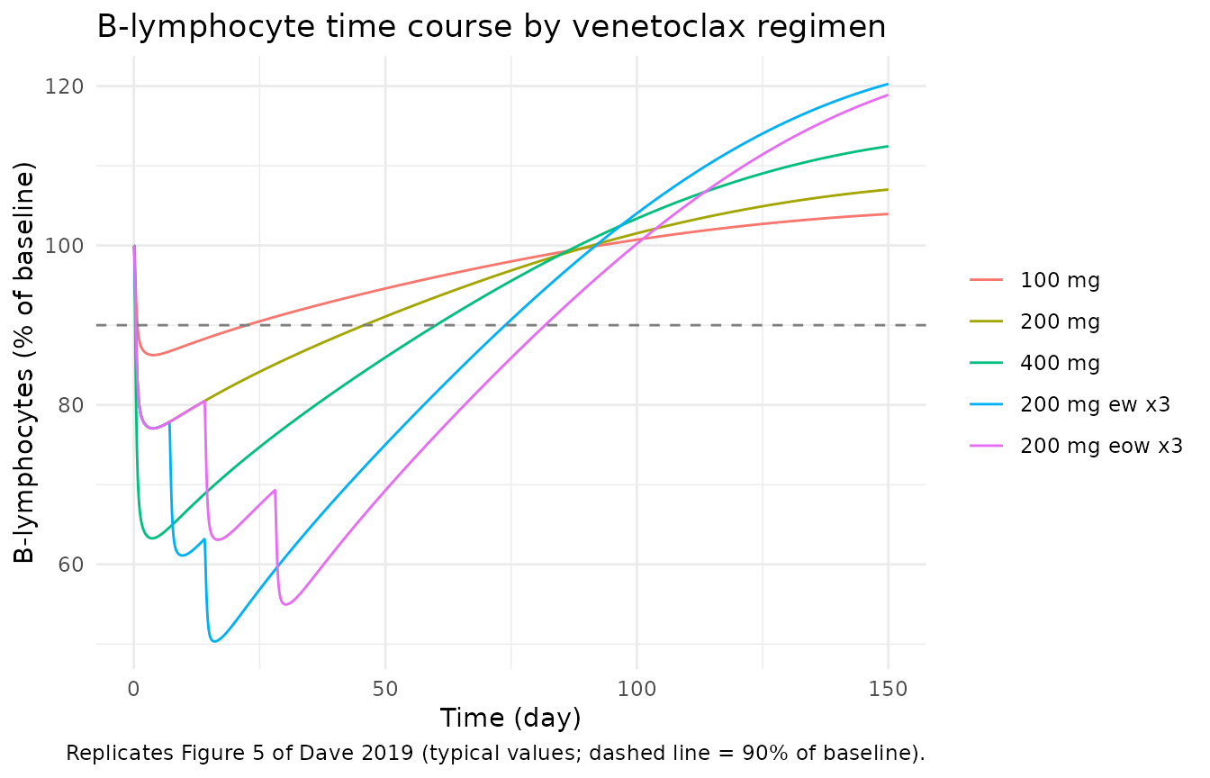
Covariate effects on exposure: exact gates
The bioavailability and clearance factors can be checked exactly. For
a linear PK model the AUC to infinity is F * Dose / CL, so
ratios of simulated AUCs must equal ratios of the Table 2 factors. The
AUCs below come from trapezoidal integration of a dense solved profile
out to 60 days, so the only error is numerical.
auc_of <- function(ev) {
  s <- solve_typical(ev)
  sum(diff(s$time) * (head(s$Cc, -1) + tail(s$Cc, -1)) / 2)
}
obs_dense <- seq(0, 60, by = 0.01)
auc_ref <- auc_of(make_events(400, food = "low", obs_times = obs_dense))
ratios <- tibble::tribble(
  ~condition, ~ev, ~expected,
  "Fasting vs low-fat", make_events(400, food = "fasted", obs_times = obs_dense), 0.29,
  "Moderate/high-fat vs low-fat", make_events(400, food = "modhigh", obs_times = obs_dense), 1.47,
  "Azithromycin", make_events(400, food = "low", azi = 1L, obs_times = obs_dense), 0.65,
  "Chinese", make_events(400, food = "low", chinese = 1L, obs_times = obs_dense), 1.53,
  "Rifampin (F x 4.91, CL x 2.67)", make_events(400, food = "low", rif = 1L, obs_times = obs_dense), 4.91 / 2.67,
  "100 mg vs 400 mg (dose-normalised)", make_events(100, food = "low", obs_times = obs_dense), (100 / 400)^-0.178 / 4
) |>
  mutate(simulated = vapply(ev, auc_of, numeric(1)) / auc_ref) |>
  select(-ev)

ratios |>
  mutate(across(c(expected, simulated), \(x) signif(x, 4))) |>
  rename(
    "Condition" = condition,
    "Expected AUC ratio" = expected,
    "Simulated AUC ratio" = simulated
  ) |>
knitr::kable(caption = "AUC ratios vs. the reference (400 mg, low-fat meal). The last row is the 100 mg AUC over the 400 mg AUC, i.e. the dose ratio 1/4 times the F ratio.")| Condition | Expected AUC ratio | Simulated AUC ratio |
|---|---|---|
| Fasting vs low-fat | 0.290 | 0.290 |
| Moderate/high-fat vs low-fat | 1.470 | 1.470 |
| Azithromycin | 0.650 | 0.650 |
| Chinese | 1.530 | 1.530 |
| Rifampin (F x 4.91, CL x 2.67) | 1.839 | 1.839 |
| 100 mg vs 400 mg (dose-normalised) | 0.320 | 0.320 |
PKNCA validation
Venetoclax concentrations were sampled up to 96 h after each dose in the pooled studies. Typical-value profiles are simulated on that window for single 100, 200 and 400 mg doses under each food condition. Time is converted to hours for reporting.
nca_grid <- expand.grid(
  dose = c(100, 200, 400), food = c("fasted", "low", "modhigh"),
  stringsAsFactors = FALSE
)
nca_grid$treatment <- paste(nca_grid$dose, "mg", nca_grid$food)
nca_grid$id <- seq_len(nrow(nca_grid))

obs_h <- sort(unique(c(seq(0, 12, by = 0.25), seq(12, 96, by = 2)))) / 24
sim_pk <- lapply(seq_len(nrow(nca_grid)), function(i) {
  ev <- make_events(
    nca_grid$dose[i], food = nca_grid$food[i], obs_times = obs_h,
    id = nca_grid$id[i]
  )
  # A single-subject solve returns no `id` column; add it back for PKNCA.
  solve_typical(ev) |> mutate(id = nca_grid$id[i], treatment = nca_grid$treatment[i])
}) |>
  bind_rows()

sim_nca <- sim_pk |>
  filter(!is.na(Cc)) |>
  transmute(id, treatment, time = time * 24, Cc)
sim_nca <- bind_rows(
  sim_nca,
  sim_nca |> distinct(id, treatment) |> mutate(time = 0, Cc = 0)
) |>
  distinct(id, treatment, time, .keep_all = TRUE) |>
  arrange(id, treatment, time)

dose_df <- nca_grid |> transmute(id, treatment, time = 0, amt = dose)

conc_obj <- PKNCA::PKNCAconc(sim_nca, Cc ~ time | treatment + id)
dose_obj <- PKNCA::PKNCAdose(dose_df, amt ~ time | treatment + id)
intervals <- data.frame(
  start = 0, end = Inf,
  cmax = TRUE, tmax = TRUE, aucinf.obs = TRUE, half.life = TRUE
)
nca_res <- PKNCA::pk.nca(PKNCA::PKNCAdata(conc_obj, dose_obj, intervals = intervals))

nca_tbl <- as.data.frame(nca_res$result) |>
  filter(PPTESTCD %in% c("cmax", "tmax", "aucinf.obs", "half.life")) |>
  select(treatment, PPTESTCD, PPORRES) |>
  pivot_wider(names_from = PPTESTCD, values_from = PPORRES)

nca_tbl |>
  mutate(across(-treatment, \(x) signif(x, 3))) |>
  rename(
    "Treatment" = treatment,
    "Cmax (mg/L)" = cmax,
    "Tmax (h)" = tmax,
    "AUC0-inf (mg*h/L)" = aucinf.obs,
    "t1/2 (h)" = half.life
  ) |>
knitr::kable(caption = "PKNCA on typical-value venetoclax profiles (0-96 h).")| Treatment | Cmax (mg/L) | Tmax (h) | t1/2 (h) | AUC0-inf (mg*h/L) |
|---|---|---|---|---|
| 100 mg fasted | 0.111 | 5.25 | 24.9 | 1.98 |
| 100 mg low | 0.383 | 6.00 | 24.8 | 6.84 |
| 100 mg modhigh | 0.563 | 6.00 | 24.8 | 10.10 |
| 200 mg fasted | 0.196 | 5.25 | 24.9 | 3.51 |
| 200 mg low | 0.677 | 6.00 | 24.8 | 12.10 |
| 200 mg modhigh | 0.995 | 6.00 | 24.8 | 17.80 |
| 400 mg fasted | 0.347 | 5.25 | 24.9 | 6.20 |
| 400 mg low | 1.200 | 6.00 | 24.8 | 21.40 |
| 400 mg modhigh | 1.760 | 6.00 | 24.8 | 31.40 |
Comparison against published NCA
Dave 2019 reports no NCA of its own. Its Introduction summarises venetoclax PK from the literature: Cmax is reached 5-8 h post-dose, and the mean terminal half-life is 17 h in healthy subjects (citing Salem 2019, Clin Pharmacokinet 58:1091). These are external reference values, so they are compared here as a check on plausibility, not as a fit target.
published_nca <- tibble::tibble(
  treatment = "400 mg low",
  tmax = 6.5, # midpoint of the quoted 5-8 h range
  half.life = 17
)
cmp <- nlmixr2lib::ncaComparisonTable(
  simulated = nca_res,
  reference = published_nca,
  by = "treatment",
  params = c("tmax", "half.life"),
  units = c(tmax = "h", half.life = "h"),
  tolerance_pct = 20
)
knitr::kable(cmp, caption = "Simulated (400 mg, low-fat) vs. literature values quoted in the Dave 2019 Introduction. * differs from reference by >20%.")| NCA parameter | treatment | Reference | Simulated | % diff |
|---|---|---|---|---|
| Tmax (h) | 400 mg low | 6.5 | 6 | -7.7% |
| t½ (h) | 400 mg low | 17 | 24.8 | +46.0%* |
The simulated Tmax (about 5-6 h across doses and food conditions) falls in the quoted 5-8 h range. The half-life estimated from the 96-h window is longer than the quoted 17 h. The 17 h figure comes from a separate NCA study, not from this model. The model’s own terminal eigenvalue is 25.2 h (from CL/F, V2/F, Q/F and V3/F in Table 2), and the NCA half-life of the simulated profile agrees with it. So the difference from 17 h lies between this population model and the separate NCA study it is being compared with, not in the simulation. The row is flagged for transparency and was not tuned.
Assumptions and deviations
-
IIV and residual error are not reported. Table 2
lists fixed effects only. The supplement’s
$OMEGA/$SIGMAblocks hold initial values, not final estimates. PK:$OMEGA BLOCK(2)0.1, 0.01, 0.1 (CL, V2), 0.1 (F1);$SIGMA0.2 (proportional), 3E-7 (additive). PD:$OMEGA0.1 (baseline);$SIGMA0.02. Under the standing policy for unreported variances, the declared random effects (etalcl,etalvc,etalfdepot,etalcirc0) and the residual SDs (propSd,addSd,expSd_circ) arefixed(0), and no value is invented. The CL-V2 covariance of the$OMEGA BLOCK(2)is not encoded either. Etas that the control streams fix to zero (on KA; and the PD ETA(2) shared by the half-life and KIN) are omitted. The model therefore gives typical-value predictions only. The paper’s reported ranges (e.g. 24% (15-35%) at 200 mg) cannot be reproduced. -
etalcirc0has nolcirc0partner. The PD baseline is the subject’s observed median pre-dose B-lymphocyte count (BLBCELL, sourceMIBTCD19) rather than an estimated theta.checkModelConventions()therefore warns thatetalcirc0has no matching fixed effect. This is deliberate and faithful toBASEB = EXP(LOG(Lymbase) + ETA(1)). - One joint model instead of the paper’s sequential fit. The paper fixed individual post hoc PK parameters (CLI, V2I, QI, V3I, KAI, F1I) before fitting the PD model. Here the PK layer drives the PD layer directly. With typical values this is the same system.
-
Lag time in the PD stage. The PD control stream
passes KAI and F1I but no
ALAG1, so its PK sub-model has no absorption lag. The packaged model keeps the PK model’s fed-state lag of 0.04 day (about 1 h) in both layers. Over a B-lymphocyte time course of weeks this difference is negligible. -
Food-effect encoding. The source
FOODcolumn (0 fasting, 1 low fat, 2 or more moderate / high fat / any meal) is mapped to the canonicalFED(FOOD >= 1) andFED_LOWFAT(FOOD == 1) indicators. The food effects on KA (THETA(6),THETA(7)) are1 FIXin the control stream and therefore omitted. -
Override order of the non-food F factors. The
control stream overwrites
TVFAin the order azithromycin, Chinese, rifampin instead of multiplying. The packaged model keeps that order. The three groups come from different studies, so they never co-occur in the source data. -
Rifampin encoding. The source flags rifampin by
study and time (
STDY.EQ.14497.AND.TIME.GE.8). That pools the single-dose (transporter inhibition) and multiple-dose (induction) phases of Study X into one indicator with effects on both CL/F and F. It is mapped toCONMED_RIFAMPICIN, not the splitCONMED_RIFAMPICIN_SD/_MDpair, because the source does not separate the phases. -
Chinese ethnicity is study-coded in the source
(Study I) and mapped to
RACE_CHINESE. -
The
1E-6inside the feedback term is kept from the control stream. It shifts the baseline steady state by a relative amount below 1e-7. -
Units. Dose is in mg and volumes in L, so
Ccis in mg/L and the drug-effect slope is in L/mg. The paper’s 38% decrease at 400 mg under moderate/high fat confirms this reading: the simulated typical value is 36.7%. The B-lymphocyte counts are in 10^6 cells/L, which equals cells/uL.