Ganciclovir renal maturation in a preterm neonate (Kata 2025)
Source:vignettes/articles/Kata_2025_ganciclovir.Rmd
Kata_2025_ganciclovir.RmdModel and source
- Citation: Kata K, Inomata S, Nishikawa M, Ide H, Nakamura K, Yoshida T, Taguchi M. Renal maturation and catch-up clearance of ganciclovir in a preterm neonate: Bayesian pharmacokinetic analysis using a population model. J Pharm Health Care Sci. 2025;11:89. doi:10.1186/s40780-025-00496-5. The sigmoid hyperbolic maturation form is cited by Kata 2025 to Anderson BJ, Holford NHG. Mechanism-based concepts of size and maturity in pharmacokinetics. Annu Rev Pharmacol Toxicol. 2008;48:303-332.
- Article (open access): https://doi.org/10.1186/s40780-025-00496-5
- PMCID: PMC12538932
Kata 2025 is a single-patient case report describing 15 weeks of ganciclovir (GCV) and valganciclovir (VGCV) therapy in a female infant born at 27 weeks 0 days gestation weighing 556 g, with congenital cytomegalovirus (CMV) infection. It contains two distinct modelling layers, and only one of them is original to the paper:
The PK layer is inherited, not re-estimated. The authors state that “Bayesian estimation was performed using the PPK model and previously reported parameters [9]”, reference 9 being Acosta 2007 (Clin Pharmacol Ther 81:867-872). They print that model in their Methods as Eqs. 1-4. It is already packaged here, independently, as
Acosta_2007_ganciclovir– so this vignette uses that model rather than shipping a second copy of it. The first validation section below is a mechanical check that the two transcriptions agree.The maturation layer is the paper’s own fit. Having obtained four phase-wise Bayesian clearance estimates, the authors normalised them to a body surface area of 1.73 m^2 and regressed them on postnatal age with a sigmoid hyperbolic (Hill) function of the Anderson and Holford form. That fit – Eq. 5 and Table 2 – is packaged here as
Kata_2025_ganciclovir_maturation.Maturation model description: Postnatal-age maturation model for ganciclovir (GCV) clearance in an extremely low birth weight preterm neonate with congenital cytomegalovirus infection (Kata 2025 J Pharm Health Care Sci). This is the paper’s only originally-estimated model: the four phase-wise Bayesian clearance estimates, obtained by re-using the Acosta 2007 neonatal ganciclovir population PK model without re-estimation (shipped here as Acosta_2007_ganciclovir), were normalised to a body surface area of 1.73 m^2 and regressed on postnatal age with a sigmoid hyperbolic (Hill) maturation function of the Anderson and Holford form, CL = cl_pna0 + cl_matspan * PNA^hill / (pna50^hill + PNA^hill). There are no compartments and no dosing: the rxode2 time axis IS postnatal age in days, and the model predicts body-surface-area normalised GCV clearance in mL/min/1.73m^2 at each observation time. The fitted curve rises from 8.80 mL/min/1.73m^2 at birth to an asymptote of 230.8, crossing the ~100 mL/min/1.73m^2 normal adult glomerular filtration rate late in the treatment course, which is the ‘catch-up’ renal maturation the paper reports.
Population
A single female infant (Kata 2025, Case presentation and Results):
- Gestational age 27 weeks 0 days at birth; birth weight 556 g (extremely low birth weight); delivered by caesarean section for non-reassuring fetal status.
- Congenital CMV confirmed by CMV DNA in urine in the early neonatal period. Blood CMV DNA fell from 2.1e6 IU/mL before GCV to 5.9e2 IU/mL by PNA 41, then plateaued.
- Body weight rose from 530 g to 2,010 g over the treatment course.
- GCV 2.5 mg/day intravenously once daily from PNA 9, increased to 3.0 mg/day once daily when the weight reached 731 g. Oral VGCV from PNA 36 at 10 then 12.5 mg/day once daily, then 15, 25 and 35 mg/day twice daily from PNA 57. VGCV was interrupted at PNA 79 for neutropenia, resumed at PNA 91, and stopped at PNA 112.
- Plasma GCV was sampled as a trough immediately before a dose and a peak 2 h after. Observed peaks 4.09, 5.34 and 3.12 ug/mL at PNA 13, 44 and 69; observed troughs 2.63, 0.64, 1.21, 0.65 and 0.60 ug/mL at PNA 16, 41, 62, 79 and 104. The peak target was 5 ug/mL.
- Assay: HPLC with fluorescence detection, linear 0.1 to 5.0 ug/mL, detection limit 0.05 ug/mL.
The inherited PK parameters come from a materially different population – Acosta 2007 studied 24 neonates aged 8 to 34 days weighing 1.9 to 4.4 kg – which Kata 2025 flags explicitly as its first limitation.
Source trace
Every parameter in ini() carries an in-file source-trace
comment. The table below collects them for review.
| Equation / parameter | Value | Source location |
|---|---|---|
| Maturation form (Eq. 5) | CL = t1 + t2 * PNA^t3 / (t4^t3 + PNA^t3) |
Methods, “Maturation analysis”, Eq. 5 (mL/min/1.73m^2) |
lcl_pna0 = log(8.80) (theta1,
mL/min/1.73m^2) |
8.80 (95% CI 8.26-9.34) | Table 2 row 1; footnote a) gives the unit |
lcl_matspan = log(222) (theta2,
mL/min/1.73m^2) |
222 (95% CI 169-274) | Table 2 row 2; footnote a) |
lhill = log(2.79) (theta3, Hill
coefficient) |
2.79 (95% CI 2.43-3.15) | Table 2 row 3 |
lpna50 = log(95.8) (theta4, days) |
95.8 (95% CI 79.5-112) | Table 2 row 4; footnote b) |
propSd = sqrt(0.0126) = 0.1122 |
omega^2 = 0.0126 (95% CI 0.00817-0.0170) | Table 2 row 5 (see Errata on the level) |
PK layer: CL = 0.146 * WT^1.68 (L/h) |
0.146, 1.68 | Methods, Eq. 1 and the sentence that follows |
PK layer: V = 1.15 (L/kg) |
1.15 | Methods, Eq. 2; Table 1 holds V at 1.15 in all phases |
PK layer: Ka = 0.591 (1/h) |
0.591 | Methods, Eq. 3 |
PK layer: F = 0.536
|
0.536 | Methods, Eq. 4 |
| Phase-wise CL, CL/F, V, F | see Table 1 | Results, Table 1 |
The PK-layer rows are the values Kata 2025 prints for the inherited
Acosta 2007 model; they are validated against the packaged
Acosta_2007_ganciclovir immediately below rather than
re-packaged.
Dimensional analysis
-
Maturation model.
cl_pna0andcl_matspanare both in mL/min/1.73m^2; the maturation factorPNA^hill / (pna50^hill + PNA^hill)is dimensionless becausePNAandpna50share units of days. The sum is therefore in mL/min/1.73m^2, matchingunits$concentration. There are no compartments and no dosing: the rxode2 time variable is postnatal age in days. -
PK layer.
CL = 0.146 * WT^1.68with WT in kg gives L/h;V = 1.15 * WTgives L. A dose in mg over a volume in L is mg/L, which is the ug/mL the paper reports. The bare (un-normalised) power on weight means the coefficient 0.146 is the clearance of a 1 kg subject, not of a cohort-median subject.
Validation 1: the inherited PK layer matches the packaged Acosta 2007 model
Kata 2025 Eqs. 1-4 and the packaged
Acosta_2007_ganciclovir were transcribed from different
secondary sources – Kata 2025 read the primary directly, while the
packaged model was transcribed from the Yang 2023 ganciclovir model
repository (Table 3). If both are faithful they must agree on all five
numbers. This check goes red if either transcription drifts.
pk_ui <- rxode2::rxode(readModelDb("Acosta_2007_ganciclovir"))
#> ℹ parameter labels from comments will be replaced by 'label()'
theta <- pk_ui$theta

packaged <- c(
  CL_coefficient = unname(exp(theta[["lcl"]])),
  WT_exponent_CL = unname(pk_ui$iniDf$est[pk_ui$iniDf$name == "e_wt_cl"]),
  V_per_kg       = unname(exp(theta[["lvc"]])),
  Ka             = unname(exp(theta[["lka"]])),
  F_oral         = unname(exp(theta[["lfdepot"]]))
)

# Values as printed in Kata 2025 Methods Eqs. 1-4 (p. 3).
kata_printed <- c(
  CL_coefficient = 0.146,
  WT_exponent_CL = 1.68,
  V_per_kg       = 1.15,
  Ka             = 0.591,
  F_oral         = 0.536
)

pk_cmp <- tibble::tibble(
  Quantity            = names(kata_printed),
  `Kata 2025 Eqs 1-4` = as.numeric(kata_printed),
  `Packaged Acosta_2007_ganciclovir` = as.numeric(packaged[names(kata_printed)])
) |>
  dplyr::mutate(Agree = abs(`Kata 2025 Eqs 1-4` -
                              `Packaged Acosta_2007_ganciclovir`) < 1e-8)

knitr::kable(pk_cmp, digits = 4)| Quantity | Kata 2025 Eqs 1-4 | Packaged Acosta_2007_ganciclovir | Agree |
|---|---|---|---|
| CL_coefficient | 0.146 | 0.146 | TRUE |
| WT_exponent_CL | 1.680 | 1.680 | TRUE |
| V_per_kg | 1.150 | 1.150 | TRUE |
| Ka | 0.591 | 0.591 | TRUE |
| F_oral | 0.536 | 0.536 | TRUE |
# Deterministic identity between two transcriptions of one source: exact.
stopifnot(nrow(pk_cmp) == 5L, all(pk_cmp$Agree))
All five agree exactly, so the packaged Acosta model is the correct PK layer for this case and no second copy is warranted.
Validation 2: Table 1 is internally consistent about bioavailability
Kata 2025 Table 1 reports CL (L/hr/kg),
CL/F (L/hr/kg) and F (%) independently for
each phase. Those three columns are over-determined: F must
equal CL / (CL/F). This confirms that the paper’s
F is the whole VGCV-to-GCV conversion carried on the oral
dose, which is how the packaged model applies it
(f(depot)).
table1 <- tibble::tibble(
  PNA_day   = c(30, 51, 72, 93),
  phase     = c("I", "II", "III", "IV"),
  CL_per_kg = c(0.048, 0.134, 0.208, 0.273),   # Table 1 row 'CL (L/hr/kg)'
  CLF_per_kg = c(NA, 0.244, 0.397, 0.522),     # Table 1 row 'CL/F (L/hr/kg)'
  V_per_kg  = c(1.15, 1.15, 1.15, 1.15),       # Table 1 row 'V (L/kg)'
  F_pct     = c(NA, 55.0, 52.4, 52.3)          # Table 1 row 'F (%)'
) |>
  dplyr::mutate(F_pct_implied = 100 * CL_per_kg / CLF_per_kg,
                abs_diff_pp   = abs(F_pct_implied - F_pct))

knitr::kable(table1, digits = 3)| PNA_day | phase | CL_per_kg | CLF_per_kg | V_per_kg | F_pct | F_pct_implied | abs_diff_pp |
|---|---|---|---|---|---|---|---|
| 30 | I | 0.048 | NA | 1.15 | NA | NA | NA |
| 51 | II | 0.134 | 0.244 | 1.15 | 55.0 | 54.918 | 0.082 |
| 72 | III | 0.208 | 0.397 | 1.15 | 52.4 | 52.393 | 0.007 |
| 93 | IV | 0.273 | 0.522 | 1.15 | 52.3 | 52.299 | 0.001 |
Validation 3: PK simulation of the case, with PKNCA
The case weight trajectory is reconstructed by linear interpolation between the three weights the paper states numerically: 556 g at birth, 530 g at the start of GCV on PNA 9 (the usual early neonatal weight loss), and 2,010 g at the end of treatment. The interpolation is checked rather than merely assumed: the paper says the GCV dose was raised from 2.5 to 3.0 mg/day when the weight reached 731 g, and that this happened during Phase I (PNA 9 to 35).
wt_at_pna <- function(pna) {
  stats::approx(x = c(0, 9, 112), y = c(0.556, 0.530, 2.010),
                xout = pna, rule = 2)$y
}

pna_at_731g <- stats::uniroot(function(p) wt_at_pna(p) - 0.731,
                              interval = c(9, 112))$root
cat(sprintf("Interpolated weight reaches 731 g at PNA %.1f days\n", pna_at_731g))
#> Interpolated weight reaches 731 g at PNA 23.0 days

# The dose increase to 3.0 mg/day must fall inside Phase I (PNA 9-35).
stopifnot(pna_at_731g > 9, pna_at_731g < 35)
Two single-dose arms are simulated at the Phase II weight to exercise
both routes: intravenous GCV into central, and oral VGCV
into depot. Typical values only (zeroRe), so
every check below is a deterministic identity rather than a draw from a
cohort.
pk_mod <- rxode2::rxode(readModelDb("Acosta_2007_ganciclovir"))
#> ℹ parameter labels from comments will be replaced by 'label()'
pk_typ <- rxode2::zeroRe(pk_mod)

wt_phase2  <- wt_at_pna(51)
dose_iv    <- 3.0    # mg GCV, the PNA-9 regimen escalated (Case presentation)
dose_oral  <- 12.5   # mg VGCV once daily (Case presentation)
obs_grid   <- sort(unique(c(seq(0, 4, by = 0.05), seq(4, 72, by = 0.25))))

build_arm <- function(amt, cmt_dose, treatment) {
  ev <- rxode2::et(amt = amt, cmt = cmt_dose, time = 0) |>
    rxode2::et(obs_grid, cmt = "central")
  ev <- as.data.frame(ev)
  ev$WT <- wt_phase2
  ev$treatment <- treatment
  ev
}

events <- dplyr::bind_rows(
  build_arm(dose_iv,   "central", "IV ganciclovir"),
  build_arm(dose_oral, "depot",   "Oral valganciclovir")
) |>
  dplyr::mutate(id = as.integer(factor(treatment)))

sim <- rxode2::rxSolve(pk_typ, events, keep = c("WT", "treatment")) |>
  as.data.frame()
#> ℹ omega/sigma items treated as zero: 'etalcl', 'etalfdepot'
#> Warning: multi-subject simulation without without 'omega'
if (is.null(sim$id)) sim$id <- 1L

cl_typ <- 0.146 * wt_phase2^1.68
vc_typ <- 1.15 * wt_phase2
cat(sprintf("Phase II weight %.3f kg -> CL %.4f L/h, V %.3f L, t1/2 %.2f h\n",
            wt_phase2, cl_typ, vc_typ, log(2) * vc_typ / cl_typ))
#> Phase II weight 1.133 kg -> CL 0.1802 L/h, V 1.304 L, t1/2 5.01 h
ggplot2::ggplot(sim, ggplot2::aes(time, Cc, colour = treatment)) +
  ggplot2::geom_line(linewidth = 0.8) +
  ggplot2::labs(x = "Time after dose (h)", y = "Plasma GCV (ug/mL)",
                colour = NULL) +
  ggplot2::theme_bw() +
  ggplot2::theme(legend.position = "top")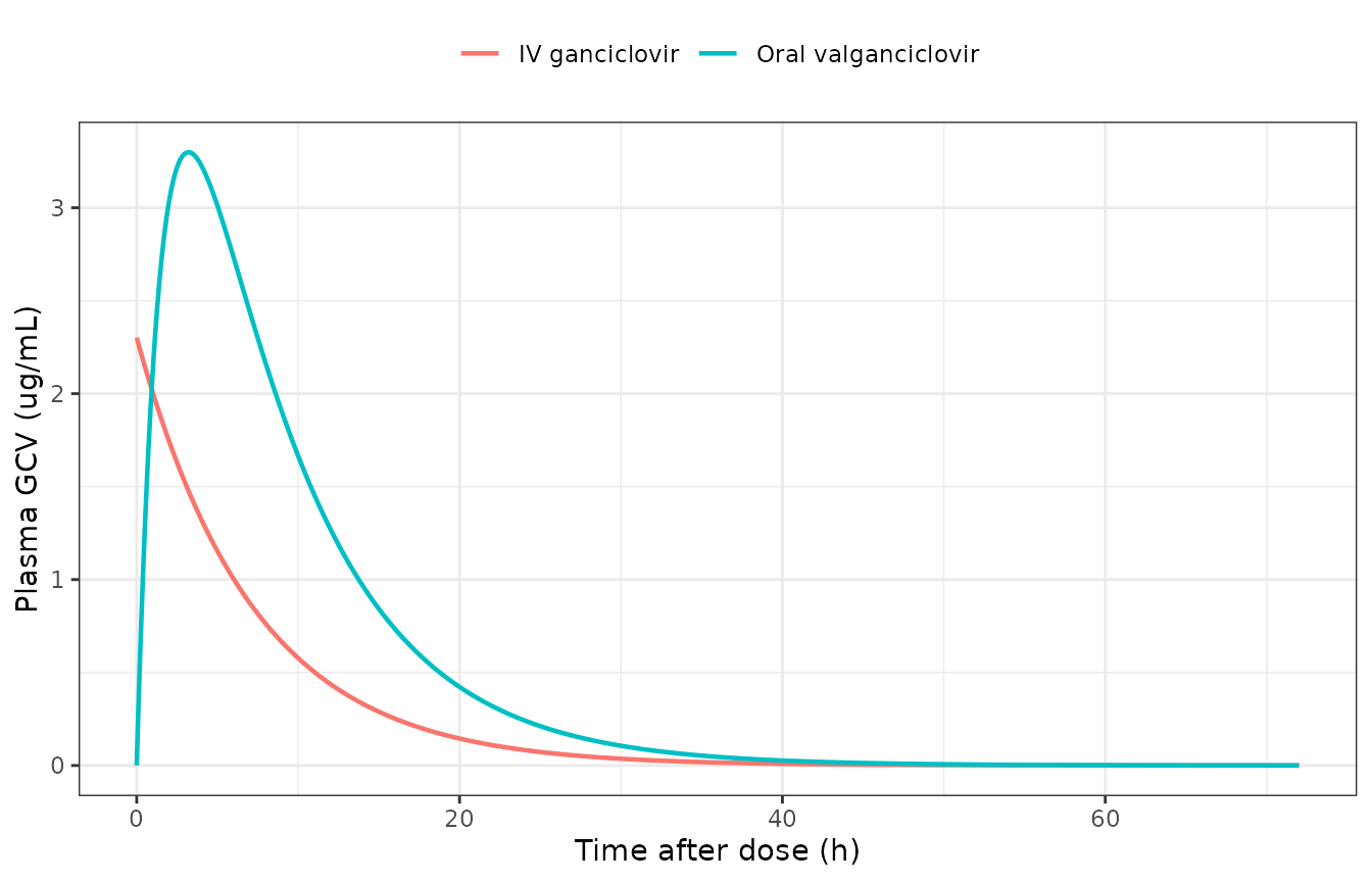
Typical-value plasma ganciclovir after a single IV ganciclovir dose and a single oral valganciclovir dose at the Phase II body weight.
Non-compartmental analysis with PKNCA, grouped by treatment arm:
conc_data <- sim |>
  dplyr::filter(!is.na(Cc)) |>
  dplyr::select(id, treatment, time, Cc)

dose_data <- tibble::tibble(
  id        = c(1L, 2L),
  treatment = c("IV ganciclovir", "Oral valganciclovir"),
  time      = 0,
  dose      = c(dose_iv, dose_oral)
)

o_conc <- PKNCA::PKNCAconc(conc_data, Cc ~ time | treatment + id,
                           concu = "ug/mL", timeu = "h")
o_dose <- PKNCA::PKNCAdose(dose_data, dose ~ time | treatment + id,
                           doseu = "mg")
o_data <- PKNCA::PKNCAdata(
  o_conc, o_dose,
  intervals = data.frame(
    start = 0, end = Inf,
    cmax = TRUE, tmax = TRUE, auclast = TRUE,
    aucinf.obs = TRUE, half.life = TRUE
  )
)
res <- suppressWarnings(PKNCA::pk.nca(o_data))
nca <- as.data.frame(res) |>
  dplyr::select(treatment, PPTESTCD, PPORRES)

knitr::kable(
  nca |>
    dplyr::filter(PPTESTCD %in% c("cmax", "tmax", "auclast",
                                  "aucinf.obs", "half.life")) |>
    tidyr::pivot_wider(names_from = PPTESTCD, values_from = PPORRES) |>
    dplyr::rename("Treatment" = treatment, "Cmax (ug/mL)" = cmax,
                  "Tmax (h)" = tmax, "AUClast (ug*h/mL)" = auclast,
                  "AUC0-inf (ug*h/mL)" = aucinf.obs, "t1/2 (h)" = half.life),
  digits = 3
)| Treatment | AUClast (ug*h/mL) | Cmax (ug/mL) | Tmax (h) | t1/2 (h) | AUC0-inf (ug*h/mL) |
|---|---|---|---|---|---|
| IV ganciclovir | 16.646 | 2.301 | 0.0 | 5.014 | 16.647 |
| Oral valganciclovir | 37.175 | 3.298 | 3.2 | 5.037 | 37.177 |
The NCA output is gated against the closed-form solutions of the
one-compartment model it came from. For an intravenous dose
AUC0-inf = Dose / CL exactly; for the oral dose the same
identity holds with the dose scaled by F, because the depot
ultimately delivers F * Dose to central.
get_nca <- function(arm, param) {
  v <- nca$PPORRES[nca$treatment == arm & nca$PPTESTCD == param]
  if (length(v) != 1L) stop("no unique ", param, " for arm '", arm, "'")
  v
}

auc_iv   <- get_nca("IV ganciclovir", "aucinf.obs")
auc_oral <- get_nca("Oral valganciclovir", "aucinf.obs")
thalf_iv <- get_nca("IV ganciclovir", "half.life")

gates <- tibble::tibble(
  Check = c(
    "IV: AUC0-inf * CL / Dose = 1",
    "Oral: AUC0-inf * CL / (F * Dose) = 1",
    "t1/2 = ln(2) * V / CL",
    "F recovered from dose-normalised AUC ratio"
  ),
  Expected = c(1, 1, log(2) * vc_typ / cl_typ, 0.536),
  Achieved = c(
    auc_iv * cl_typ / dose_iv,
    auc_oral * cl_typ / (0.536 * dose_oral),
    thalf_iv,
    (auc_oral / dose_oral) / (auc_iv / dose_iv)
  )
) |>
  dplyr::mutate(`Relative error` = abs(Achieved - Expected) / Expected)

knitr::kable(gates, digits = 5)| Check | Expected | Achieved | Relative error |
|---|---|---|---|
| IV: AUC0-inf * CL / Dose = 1 | 1.00000 | 1.00000 | 0e+00 |
| Oral: AUC0-inf * CL / (F * Dose) = 1 | 1.00000 | 0.99995 | 5e-05 |
| t1/2 = ln(2) * V / CL | 5.01378 | 5.01378 | 0e+00 |
| F recovered from dose-normalised AUC ratio | 0.53600 | 0.53597 | 5e-05 |
Validation 4: the maturation model reproduces Table 2 and the Results text
The maturation model has no dosing and no compartments;
time is postnatal age in days.
mat_mod <- readModelDb("Kata_2025_ganciclovir_maturation")

# 95.8 is theta4 and 30/51/72/93 are the phase ages; include them explicitly
# so the lookups below land exactly on a solved point rather than interpolating.
pna_grid <- sort(unique(c(seq(0, 140, by = 0.5), 95.8, 30, 51, 72, 93)))
mat_sim <- rxode2::rxSolve(mat_mod, rxode2::et(pna_grid)) |>
  as.data.frame()

at_pna <- function(p) {
  v <- mat_sim$CL_bsa[match(p, mat_sim$time)]
  if (anyNA(v)) stop("PNA value(s) not on the simulation grid")
  v
}
theta1 <- 8.80; theta2 <- 222; theta3 <- 2.79; theta4 <- 95.8
hand <- function(p) theta1 + theta2 * p^theta3 / (theta4^theta3 + p^theta3)

phase_pna <- c(30, 51, 72, 93)

mat_checks <- tibble::tibble(
  Check = c(
    "CL at PNA 0 equals theta1 (the intercept)",
    "CL at PNA = theta4 equals theta1 + theta2/2 (half maturation)",
    "CL approaches theta1 + theta2 as PNA grows without bound",
    "Late-phase CL exceeds 100 mL/min/1.73m^2 (Results)",
    "Solved curve equals Eq. 5 evaluated by hand at the four phase ages"
  ),
  Expected = c(sprintf("%.2f", c(theta1, theta1 + theta2 / 2,
                                 theta1 + theta2)), "TRUE", "TRUE"),
  Achieved = c(
    sprintf("%.2f", c(at_pna(0), at_pna(theta4), hand(1e5))),
    as.character(at_pna(93) > 100),
    as.character(max(abs(at_pna(phase_pna) - hand(phase_pna))) < 1e-8)
  )
)
knitr::kable(mat_checks, digits = 4)| Check | Expected | Achieved |
|---|---|---|
| CL at PNA 0 equals theta1 (the intercept) | 8.80 | 8.80 |
| CL at PNA = theta4 equals theta1 + theta2/2 (half maturation) | 119.80 | 119.80 |
| CL approaches theta1 + theta2 as PNA grows without bound | 230.80 | 230.80 |
| Late-phase CL exceeds 100 mL/min/1.73m^2 (Results) | TRUE | TRUE |
| Solved curve equals Eq. 5 evaluated by hand at the four phase ages | TRUE | TRUE |
stopifnot(
  # Deterministic algebra, so these are exact identities, not tolerances
  # chosen from a run.
  abs(at_pna(0) - theta1) < 1e-8,
  abs(at_pna(theta4) - (theta1 + theta2 / 2)) < 1e-8,
  abs(hand(1e5) - (theta1 + theta2)) < 1e-3,
  max(abs(at_pna(phase_pna) - hand(phase_pna))) < 1e-8,
  # Maturation is monotone and has not yet plateaued inside the observed
  # window: at the end of the 140-day grid the curve has covered 74.2% of
  # its span, which is why the paper describes maturation as ongoing.
  all(diff(mat_sim$CL_bsa) > 0),
  at_pna(140) < theta1 + theta2,
  abs((at_pna(140) - theta1) / theta2 - 0.742) < 0.01,
  # The Results claim.
  at_pna(93) > 100
)

phase_tab <- tibble::tibble(
  Phase = c("I", "II", "III", "IV"),
  `PNA (days)` = phase_pna,
  `CL (mL/min/1.73m^2)` = at_pna(phase_pna)
)
knitr::kable(phase_tab, digits = 2)| Phase | PNA (days) | CL (mL/min/1.73m^2) |
|---|---|---|
| I | 30 | 17.17 |
| II | 51 | 41.42 |
| III | 72 | 77.78 |
| IV | 93 | 115.21 |
ggplot2::ggplot(mat_sim, ggplot2::aes(time, CL_bsa)) +
  ggplot2::geom_line(linewidth = 0.9) +
  ggplot2::geom_hline(yintercept = 100, linetype = "dashed",
                      colour = "grey40") +
  ggplot2::geom_point(data = phase_tab,
                      ggplot2::aes(`PNA (days)`, `CL (mL/min/1.73m^2)`),
                      size = 2.6) +
  ggplot2::annotate("text", x = 4, y = 105,
                    label = "normal GFR", hjust = 0, size = 3,
                    colour = "grey30") +
  ggplot2::labs(x = "Postnatal age (days)",
                y = "GCV clearance (mL/min/1.73m^2)") +
  ggplot2::theme_bw()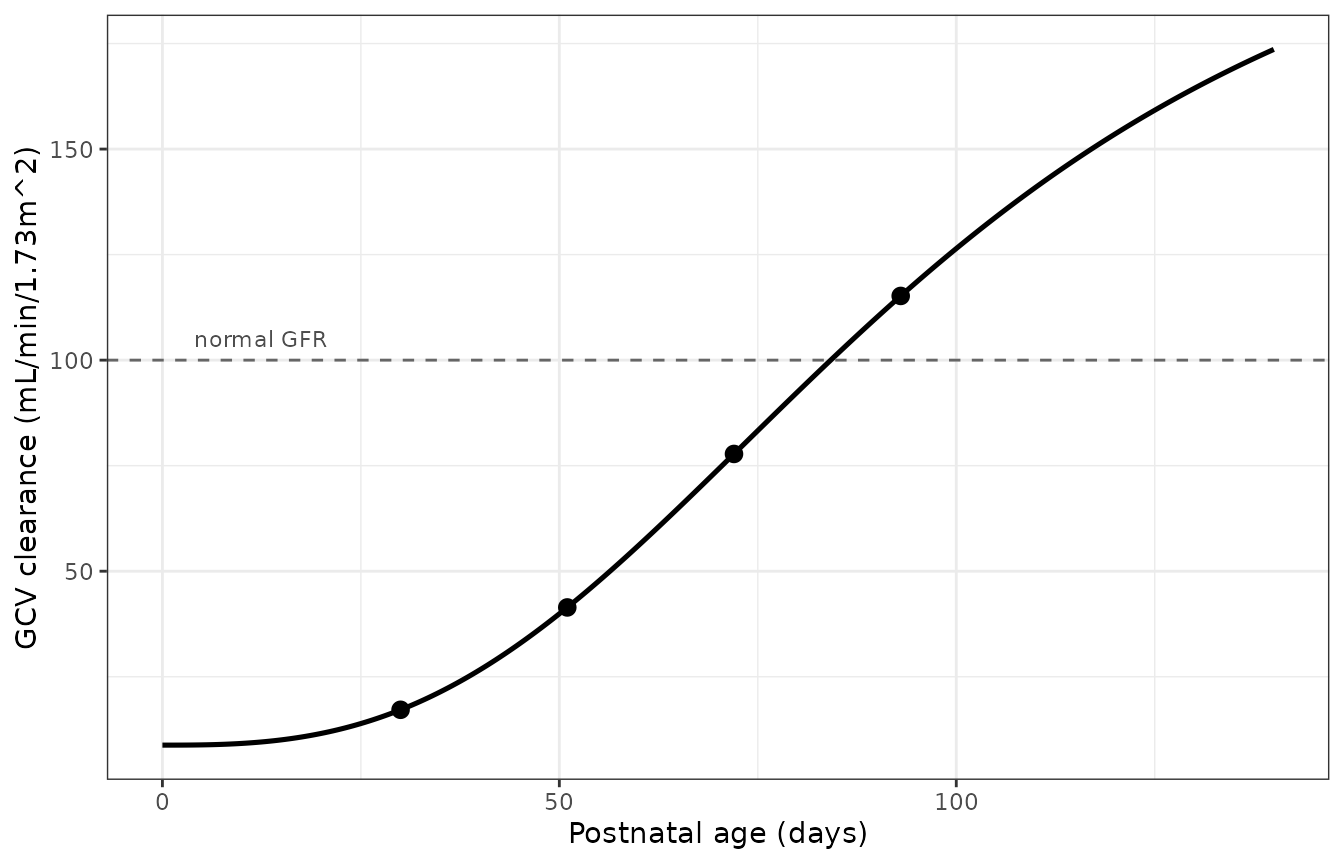
Replicates Figure 2 of Kata 2025: modelled GCV clearance (solid line) rising over postnatal age, with the four phase-wise estimates marked. The dashed line is 100 mL/min/1.73m^2, approximately the normal adult glomerular filtration rate, which the curve crosses late in the treatment course.
Validation 5: the two layers are mutually consistent
Table 1 reports clearance per kilogram of body weight; Table 2 reports it per 1.73 m^2 of body surface area. The two are linked by the subject’s BSA, which the paper does not tabulate. Dividing one by the other therefore implies a BSA at each phase, and that implied value is an independent check: it must be physiologically sensible for a neonate of the corresponding weight.
link <- tibble::tibble(
  Phase = c("I", "II", "III", "IV"),
  PNA   = phase_pna,
  WT_kg = wt_at_pna(phase_pna),
  CL_per_kg_Lh = c(0.048, 0.134, 0.208, 0.273),      # Table 1
  CL_bsa       = at_pna(phase_pna)                   # Table 2 model
) |>
  dplyr::mutate(
    CL_absolute_mL_min = CL_per_kg_Lh * WT_kg * 1000 / 60,
    BSA_implied_m2     = 1.73 * CL_absolute_mL_min / CL_bsa,
    # Meeh / Haycock-type neonatal BSA for comparison, from weight alone.
    BSA_haycock_like   = 0.1 * WT_kg^(2 / 3)
  )

knitr::kable(link, digits = 4)| Phase | PNA | WT_kg | CL_per_kg_Lh | CL_bsa | CL_absolute_mL_min | BSA_implied_m2 | BSA_haycock_like |
|---|---|---|---|---|---|---|---|
| I | 30 | 0.8317 | 0.048 | 17.1718 | 0.6654 | 0.0670 | 0.0884 |
| II | 51 | 1.1335 | 0.134 | 41.4175 | 2.5315 | 0.1057 | 0.1087 |
| III | 72 | 1.4352 | 0.208 | 77.7770 | 4.9755 | 0.1107 | 0.1272 |
| IV | 93 | 1.7370 | 0.273 | 115.2094 | 7.9033 | 0.1187 | 0.1445 |
# A neonate between 0.5 and 2 kg has a BSA of roughly 0.06 to 0.16 m^2.
# This is a wide, absolute, physiologically-grounded window, not a bound
# tuned to one run -- it goes red on a unit error in either table.
stopifnot(all(link$BSA_implied_m2 > 0.04),
          all(link$BSA_implied_m2 < 0.20))

# The implied BSA must also track weight in the right direction.
stopifnot(link$BSA_implied_m2[4] > link$BSA_implied_m2[1])
The implied body surface areas sit in the expected neonatal range and grow with weight, so the per-kg and per-1.73m^2 clearances describe the same subject.
Validation 6: which weight exponent reproduces the paper’s own Bayesian fit
Kata 2025 states the inherited clearance equation twice with two
different exponents: the Methods print CL = 0.146 * WT^1.68
(Eq. 1, restated in the following sentence), while the Introduction
restates the same Acosta 2007 model as
CL = 0.146 * WT^1.18. The packaged
Acosta_2007_ganciclovir, transcribed independently from the
Yang 2023 repository, gives 1.68, which settles the question 2 to 1. The
paper’s own Bayesian estimates agree: a Bayesian posterior shrinks
toward its prior, so the reading that produces the smaller
deviation between the individual estimates and the population prediction
is the prior that was actually used.
wt_phase <- wt_at_pna(phase_pna)
cl_ind   <- c(0.048, 0.134, 0.208, 0.273)   # Table 1, L/h/kg

eta_span <- function(b) {
  cl_pop <- 0.146 * wt_phase^b / wt_phase   # population CL per kg
  diff(range(log(cl_ind / cl_pop)))
}

exp_cmp <- tibble::tibble(
  `Weight exponent` = c(1.68, 1.18),
  Source = c("Methods Eq. 1 + Yang 2023 repository",
             "Introduction prose only"),
  `Span of implied eta` = c(eta_span(1.68), eta_span(1.18))
)
knitr::kable(exp_cmp, digits = 3)| Weight exponent | Source | Span of implied eta |
|---|---|---|
| 1.68 | Methods Eq. 1 + Yang 2023 repository | 1.238 |
| 1.18 | Introduction prose only | 1.606 |
# The Methods/repository reading must require less shrinkage than the
# Introduction reading. This is arithmetic on printed values, not a draw.
stopifnot(eta_span(1.68) < eta_span(1.18))
Assumptions and deviations
-
The PK layer is not re-packaged. Kata 2025 re-used
the Acosta 2007 model without re-estimation, and all five of its printed
values match the already-packaged
Acosta_2007_ganciclovirexactly (Validation 1). Shipping a second file would have added a duplicate that was strictly less complete, since Kata 2025 does not report the Acosta IIV or residual-error magnitudes while the packaged model carries them. This vignette therefore usesAcosta_2007_ganciclovirfor every PK simulation, and only the maturation fit is new. -
Weight exponent 1.68, not 1.18. See Validation 6.
The Introduction sentence carrying 1.18 is independently unreliable: it
also says “WT is body weight in grams”, under which its own companion
equation
V = 1.15 * WTwould give a volume of distribution near 1,150 L. Recorded as an erratum rather than silently resolved. -
The variance level is a convention, not a finding.
Table 2 reports a single
omega^2of 0.0126. The Methods describe it as “a proportional error model incorporating a random variable eta”, while the Table 2 footnote calls it “an interindividual variance”. With one subject the two levels are not identifiable. It is encoded as a proportional residual (propSd = sqrt(0.0126) = 0.1122) per the Methods sentence, which is the one that actually describes the error structure. A user who wants the footnote’s reading can move the same number to anetalcl_pna0. -
Observation name
CL_bsa.checkModelConventions()warns that a single-output model should observeCc. That canonical is for drug concentrations; this model’s observable is a body-surface-area normalised clearance in mL/min/1.73m^2, soCcwould misname it. The warning is accepted deliberately. - Weight trajectory is interpolated, not digitised. Only three weights are given numerically (556 g at birth, 530 g at PNA 9, 2,010 g at the end); Fig. 1 panel b plots the rest. Linear interpolation between the stated anchors is used, and is checked against the paper’s statement that the dose rose when the weight reached 731 g (Validation 3). Any quantity derived from the trajectory – the implied BSAs of Validation 5 and the eta spans of Validation 6 – inherits that approximation, which is why those checks use wide absolute windows and an ordering comparison rather than tight numeric targets.
- Twice-daily dose amounts. The paper writes regimens as “15 mg/day twice daily”, so the stated number is read as the total daily dose split across two administrations. This affects none of the checks above, which use the single-dose once-daily regimens.
-
Only four points support five parameters. The
maturation regression is fitted to four phase-wise clearance estimates
plus two 24-h-urine creatinine clearance reference values. The
confidence intervals in Table 2 are the authors’
estimate +/- 1.96 * SEand are reproduced here for provenance only; they are not used by the model. - Acosta 2007 remains unobtained. The primary (PMID 17392728) is not open access. Both packaged transcriptions of it are secondary – via Yang 2023 and via Kata 2025 – and they agree, but neither is the primary.