Fosfomycin calcium (Isla 2024) • nlmixr2lib

Model and source

ui <- rxode2::rxode(readModelDb("Isla_2024_fosfomycinCalcium"))
#> ℹ parameter labels from comments will be replaced by 'label()'
#> Warning: some etas defaulted to non-mu referenced, possible parsing error: etaiov_cl_1, etaiov_cl_2, etaiov_cl_3, etaiov_cl_4, etaiov_vc_1, etaiov_vc_2, etaiov_vc_3, etaiov_vc_4
#> as a work-around try putting the mu-referenced expression on a simple line

Citation: Isla A, Alarcia-Lacalle A, Solinis MA, del Pozo-Rodriguez A, Abajo Z, Cabero M, Canut-Blasco A, Rodriguez-Gascon A. Population pharmacokinetics of oral fosfomycin calcium in healthy women. J Antimicrob Chemother. 2024;79(11):2891-2898. doi:10.1093/jac/dkae295.
Article: https://doi.org/10.1093/jac/dkae295
PubMed Central: https://www.ncbi.nlm.nih.gov/pmc/articles/PMC11531824/

Two-compartment population PK model with first-order absorption and an absorption lag time for oral fosfomycin calcium (Fosfocina) in 24 healthy adult women studied in a four-period randomized crossover bioavailability trial (500 mg capsule single dose, 1000 mg capsule single dose, 1000 mg oral suspension single dose, and 1000 mg capsules every 8 h for 3 days). All disposition parameters are apparent (CL/F, V1/F, Q/F, V2/F) because no intravenous arm was studied, so absolute bioavailability is not identifiable and F is absorbed into every volume and clearance term. Three covariate-parameter relationships are retained: raw Cockcroft-Gault creatinine clearance on CL/F as an exponential centered at the 108 mL/min cohort median, body weight on V1/F as a linear ratio to the 64 kg cohort median, and the oral-suspension formulation on both the absorption rate constant (1.17-fold faster than capsules) and the absorption lag time (0.84-fold, i.e. shorter, than capsules). Inter-individual variability is diagonal on CL/F, V1/F, ka and the lag time; inter-occasion variability across the four crossover periods is carried on CL/F and V1/F and is larger than the corresponding IIV for both. Residual error is combined additive plus proportional. Absorption is markedly rate-limiting (ka = 0.15 1/h against kel = CL/V1 = 0.97 1/h), so the disposition is flip-flop and the apparent terminal slope is governed by ka (Isla 2024).

Population

Isla 2024 studied 24 healthy adult women at a single Spanish centre (Clinical Trial Unit, Araba University Hospital, Vitoria-Gasteiz; AEMPS code PD7522.22, EudraCT 2020-001664-28) in an open-label randomized four-period crossover bioavailability trial of oral fosfomycin calcium (Fosfocina). Each woman received all four treatments in a randomized sequence with a washout exceeding one week between periods: a single 500 mg capsule dose, a single 1000 mg capsule dose, a single 1000 mg oral-suspension dose (20 mL of a 250 mg/5 mL product), and 1000 mg capsules every 8 h for 3 days with sampling after the last dose. All doses were taken fasted with 200 mL of water.

Baseline demographics (Isla 2024 Table 1) are tightly clustered, as is usual for a healthy-volunteer bioavailability study: age 19-49 years (mean 32), weight 51.7-94.8 kg (mean 65.1, median 64.3), BMI 20.0-29.9 kg/m^2, serum creatinine 0.64-0.92 mg/dL, and Cockcroft-Gault creatinine clearance 82.9-158.4 mL/min (mean 109.4, median 108.0). Women with renal failure and women with a BMI at or above 30 kg/m^2 were excluded, so both retained covariates are fitted over a narrow, healthy range and the paper’s own Discussion cautions against extrapolating to renal impairment or obesity.

Thirteen plasma samples were drawn per subject per period (pre-dose and 1, 1.5, 2, 2.5, 3, 3.5, 4, 4.5, 6, 8, 12 and 24 h), giving 1124 concentration records for model building. Four women were excluded from the multiple-dose period for dosing or sampling deviations, leaving n = 20 there. Fosfomycin was assayed by HPLC-MS/MS, linear from 50 ng/mL to 50000 ng/mL. The model was fitted in NONMEM 7.4 with FOCE-INTER and evaluated by pcVPC and by a 1000-sample bootstrap (919 successful runs).

str(ui$population)
#> List of 13
#>  $ species         : chr "human"
#>  $ n_subjects      : int 24
#>  $ n_studies       : int 1
#>  $ n_observations  : int 1124
#>  $ age_range       : chr "19-49 years (mean 32, median 32, SD 9); protocol eligibility 18-55 years"
#>  $ weight_range    : chr "51.7-94.8 kg (mean 65.1, median 64.3, SD 9.6)"
#>  $ sex_female_pct  : num 100
#>  $ disease_state   : chr "Healthy adult women volunteers with no evidence of significant organic or psychiatric disease, normal clinical "| __truncated__
#>  $ renal_function  : chr "Uniformly normal to mildly augmented. Serum creatinine 0.64-0.92 mg/dL (mean 0.77); Cockcroft-Gault creatinine "| __truncated__
#>  $ hepatic_function: chr "Normal. GOT 13-34 U/L, GPT 6-54 U/L, GGT 9-40 U/L, total plasma proteins 6.3-7.6 g/dL (Isla 2024 Table 1). Tran"| __truncated__
#>  $ dose_range      : chr "Four treatments per subject in a randomized crossover with washout exceeding one week between periods: (i) 500 "| __truncated__
#>  $ regions         : chr "Spain (single centre: Clinical Trial Unit, Araba University Hospital, Vitoria-Gasteiz)."
#>  $ notes           : chr "Regulatory identifiers: AEMPS code PD7522.22, EudraCT 2020-001664-28. Thirteen plasma samples per subject per p"| __truncated__

Source trace

Every value below carries the same citation as an in-file comment beside its ini() entry in inst/modeldb/specificDrugs/Isla_2024_fosfomycinCalcium.R. All disposition parameters are apparent (divided by the unknown oral bioavailability F): the trial had no intravenous arm.

Equation / parameter	Value	Source location
`lcl` = log(CL/F) at CRCL 108 mL/min	23.7 L/h	Table 2, `theta_CL` (RSE 5%); Results text “the estimated CL/F value for a woman with CLCR of 108 mL/min is 23.7 L/h”
`e_crcl_cl`	0.0060 (mL/min)^-1	Table 2, `theta_CLCR` (RSE 38%), in `CL/F = theta_CL * e^(theta_CLCR * (CLCR - 108))`
`lvc` = log(V1/F) at 64 kg	24.4 L	Table 2, `theta_V1` (RSE 14%); Results text “the typical value for V1/F … 24.4 L”
`e_wt_vc`	1 (fixed)	Table 2, `V1/F (L) = theta_V1 * (BW/64)` – the ratio enters to the first power; no exponent is estimated
`lq` = log(Q/F)	4.04 L/h	Table 2, `theta_Q` (RSE 24%); Results text “inter-compartmental clearance (Q/F) … 4.04 L/h”
`lvp` = log(V2/F) at 64 kg	24.4 x 4.94 = 120.536 L	Table 2, `theta_V2` = 4.94 (RSE 38%) as the V2/V1 ratio in `Vss/F = (V1 * (1 + theta_V2))`
`e_wt_vp`	1 (fixed)	Inherited from `lvc` through the `V2 = V1 * theta_V2` ratio parameterisation
`lka` = log(ka), capsule	0.15 1/h	Table 2, `theta_KA1` (RSE 10%)
`e_form_syrup_ka`	log(1.17)	Table 2, `theta_KA2` (RSE 9%), in `KA (suspension) = theta_KA1 x theta_KA2`
`ltlag` = log(TLAG), capsule	0.84 h	Table 2, `theta_TLAG1` (RSE 2%)
`e_form_syrup_tlag`	log(0.84)	Table 2, `theta_TLAG2` (RSE 5%), in `TLAG (suspension) = theta_TLAG1 x theta_TLAG2`
`etalcl`	log(1 + 0.157^2)	Table 2, “IIV on CL/F (%)” = 15.7 (RSE 27%, eta-shrinkage 34%)
`etalvc`	log(1 + 0.294^2)	Table 2, “IIV on V1/F (%)” = 29.4 (RSE 47%, eta-shrinkage 43%)
`etalka`	log(1 + 0.327^2)	Table 2, “IIV on KA (%)” = 32.7 (RSE 18%, eta-shrinkage 6.0%)
`etaltlag`	log(1 + 0.048^2)	Table 2, “IIV on TLAG (%)” = 4.8 (RSE 34%, eta-shrinkage 44%)
`etaiov_cl_*`	log(1 + 0.346^2)	Table 2, “IOV on CL/F (%)” = 34.6 (RSE 10%)
`etaiov_vc_*`	log(1 + 0.667^2)	Table 2, “IOV on V1/F (%)” = 66.7 (RSE 14%)
`addSd`	0.209 mg/L	Table 2, “RE additive (mg/L)” (RSE 17%, eps-shrinkage 8%)
`propSd`	0.199	Table 2, “RE proportional (%)” (RSE 8%) – the value is the NONMEM fraction 19.9%; see Errata
Two-compartment ODEs with first-order absorption and lag	n/a	Results “Base model”: “the two-compartment model with first order absorption and elimination improved the fit … The inclusion of an absorption lag time (TLAG) significantly improved the fitting”
Combined additive + proportional residual	n/a	Methods “Population PK modelling”; Table 2 reports one row of each

Structural checks against the paper’s own printed values

The paper prints several derived quantities that over-determine the parameter table, so the transcription can be checked without any simulation at all. These are deterministic identities – no random draw is involved – so they carry tight tolerances.

ev_ref <- rxode2::et(amt = 1000, cmt = "depot") |>
  rxode2::et(seq(0, 24, by = 0.05), cmt = "central")

solve_typical <- function(form_syrup, crcl = 108, wt = 64, ev = ev_ref) {
  d <- as.data.frame(ev)
  d$CRCL <- crcl
  d$WT <- wt
  d$FORM_SYRUP <- form_syrup
  d$OCC <- 1
  rxode2::rxSolve(
    rxode2::zeroRe(readModelDb("Isla_2024_fosfomycinCalcium")),
    d,
    omega = NA, sigma = NA, returnType = "data.frame"
  )
}

cap <- solve_typical(0)
#> ℹ parameter labels from comments will be replaced by 'label()'
#> Warning: some etas defaulted to non-mu referenced, possible parsing error: etaiov_cl_1, etaiov_cl_2, etaiov_cl_3, etaiov_cl_4, etaiov_vc_1, etaiov_vc_2, etaiov_vc_3, etaiov_vc_4
#> as a work-around try putting the mu-referenced expression on a simple line
#> Warning: some etas defaulted to non-mu referenced, possible parsing error: etaiov_cl_1, etaiov_cl_2, etaiov_cl_3, etaiov_cl_4, etaiov_vc_1, etaiov_vc_2, etaiov_vc_3, etaiov_vc_4
#> as a work-around try putting the mu-referenced expression on a simple line
#> Warning: some etas defaulted to non-mu referenced, possible parsing error: etaiov_cl_1, etaiov_cl_2, etaiov_cl_3, etaiov_cl_4, etaiov_vc_1, etaiov_vc_2, etaiov_vc_3, etaiov_vc_4
#> as a work-around try putting the mu-referenced expression on a simple line
sus <- solve_typical(1)
#> ℹ parameter labels from comments will be replaced by 'label()'
#> Warning: some etas defaulted to non-mu referenced, possible parsing error: etaiov_cl_1, etaiov_cl_2, etaiov_cl_3, etaiov_cl_4, etaiov_vc_1, etaiov_vc_2, etaiov_vc_3, etaiov_vc_4
#> as a work-around try putting the mu-referenced expression on a simple line
#> Warning: some etas defaulted to non-mu referenced, possible parsing error: etaiov_cl_1, etaiov_cl_2, etaiov_cl_3, etaiov_cl_4, etaiov_vc_1, etaiov_vc_2, etaiov_vc_3, etaiov_vc_4
#> as a work-around try putting the mu-referenced expression on a simple line

structural <- tibble::tribble(
  ~Quantity,                          ~Source,                        ~Published, ~Model,
  "CL/F at CRCL 108 mL/min (L/h)",    "Table 2 / Results text",        23.7,      cap$cl[1],
  "V1/F at 64 kg (L)",                "Table 2 / Results text",        24.4,      cap$vc[1],
  "Q/F (L/h)",                        "Table 2 / Results text",         4.04,     cap$q[1],
  "Vss/F = V1/F * (1 + theta_V2) (L)","Results text; Discussion 144.94",144.9,    cap$vc[1] + cap$vp[1],
  "KA, capsule (1/h)",                "Table 2 theta_KA1",              0.15,     cap$ka[1],
  "KA, suspension (1/h)",             "Table 2 printed sub-row",        0.18,     sus$ka[1],
  "TLAG, capsule (h)",                "Table 2 theta_TLAG1",            0.84,     cap$tlag[1],
  "TLAG, suspension (h)",             "Table 2 printed sub-row",        0.70,     sus$tlag[1]
) |>
  dplyr::mutate(`% diff` = 100 * (Model - Published) / Published)

knitr::kable(structural, digits = 3,
             caption = "Model typical values against the values Isla 2024 prints in Table 2 and in the Results text.")

Model typical values against the values Isla 2024 prints in Table 2 and in the Results text.
Quantity	Source	Published	Model	% diff
CL/F at CRCL 108 mL/min (L/h)	Table 2 / Results text	23.70	23.700	0.000
V1/F at 64 kg (L)	Table 2 / Results text	24.40	24.400	0.000
Q/F (L/h)	Table 2 / Results text	4.04	4.040	0.000
Vss/F = V1/F * (1 + theta_V2) (L)	Results text; Discussion 144.94	144.90	144.936	0.025
KA, capsule (1/h)	Table 2 theta_KA1	0.15	0.150	0.000
KA, suspension (1/h)	Table 2 printed sub-row	0.18	0.176	-2.500
TLAG, capsule (h)	Table 2 theta_TLAG1	0.84	0.840	0.000
TLAG, suspension (h)	Table 2 printed sub-row	0.70	0.706	0.800


# The two suspension sub-rows are DERIVED products of two values that Table 2
# prints to only two decimal places, so they can only be matched to that
# precision: 0.15 * 1.17 = 0.1755 against a printed 0.18 (-2.5%) and
# 0.84 * 0.84 = 0.7056 against a printed 0.70 (+0.8%). Both discrepancies sit
# well inside the rounding interval of the underlying estimates -- a theta_TLAG
# pair anywhere in [0.835, 0.845] rounds to 0.84 and squares to 0.697-0.714 --
# so 3% is the tightest bound the source's own precision supports. Every other
# row is an exact identity and is gated at 0.05%.
derived_rows <- structural$Quantity %in% c("KA, suspension (1/h)", "TLAG, suspension (h)")
stopifnot(
  abs(structural$`% diff`[!derived_rows]) < 0.05,
  abs(structural$`% diff`[derived_rows]) < 3
)

The absorption rate constant for the capsule (0.15 1/h) is far below the elimination rate constant kel = CL/F / V1/F:

kel_ref <- cap$cl[1] / cap$vc[1]
c(ka = cap$ka[1], kel = kel_ref, ratio = kel_ref / cap$ka[1])
#>        ka       kel     ratio 
#> 0.1500000 0.9713115 6.4754098
stopifnot(cap$ka[1] < kel_ref / 3)

so absorption is rate-limiting and the profile is flip-flop: the apparent terminal slope tracks ka, not elimination. This is why the observed concentration-time curves in Isla 2024 Figure 1 decline slowly out to 24 h despite an apparent clearance of 23.7 L/h, and it is the reason the multiple-dose arm accumulates as much as it does.

Replicating Table 3 – the paper’s own covariate simulation

Isla 2024 Table 3 reports CL/F and V1/F for cohorts of 2000 virtual women at three body weights (55, 64, 90 kg) and three creatinine clearances (80, 108, 150 mL/min). The table gives both a median and a mean (SD) per cell. Because the covariate models are deterministic given the covariate value, the medians are exactly the model’s typical values; and because the random effects are log-normal, the means sit above the medians by exactly exp(sum(omega^2) / 2) over the IIV and IOV variances that apply to each parameter. Both columns are therefore reproducible without simulating anything, which makes Table 3 a strong falsifier for the whole encoding – the covariate functional forms, the centring constants, and the %CV-versus-variance reading of the random-effect rows all have to be right simultaneously.

# Pull the random-effect variances straight out of the packaged model so this
# check reads the file under test, not a hand-copied constant.
omegas <- ui$iniDf |>
  dplyr::filter(!is.na(neta1), neta1 == neta2) |>
  dplyr::select(name, est)
omega_of <- function(nm) {
  v <- omegas$est[omegas$name == nm]
  if (length(v) != 1L) stop("no unique omega for '", nm, "'")
  v
}

# Log-normal mean/median ratio for each parameter: exp(sum of its variances / 2).
infl_cl <- exp((omega_of("etalcl") + omega_of("etaiov_cl_1")) / 2)
infl_vc <- exp((omega_of("etalvc") + omega_of("etaiov_vc_1")) / 2)
c(CL = infl_cl, V1 = infl_vc)
#>       CL       V1 
#> 1.071128 1.252908

crcl_grid <- c(80, 108, 150)
cl_med <- vapply(crcl_grid, function(x) solve_typical(0, crcl = x)$cl[1], numeric(1))
#> ℹ parameter labels from comments will be replaced by 'label()'
#> Warning: some etas defaulted to non-mu referenced, possible parsing error: etaiov_cl_1, etaiov_cl_2, etaiov_cl_3, etaiov_cl_4, etaiov_vc_1, etaiov_vc_2, etaiov_vc_3, etaiov_vc_4
#> as a work-around try putting the mu-referenced expression on a simple line
#> Warning: some etas defaulted to non-mu referenced, possible parsing error: etaiov_cl_1, etaiov_cl_2, etaiov_cl_3, etaiov_cl_4, etaiov_vc_1, etaiov_vc_2, etaiov_vc_3, etaiov_vc_4
#> as a work-around try putting the mu-referenced expression on a simple line
#> ℹ parameter labels from comments will be replaced by 'label()'
#> Warning: some etas defaulted to non-mu referenced, possible parsing error: etaiov_cl_1, etaiov_cl_2, etaiov_cl_3, etaiov_cl_4, etaiov_vc_1, etaiov_vc_2, etaiov_vc_3, etaiov_vc_4
#> as a work-around try putting the mu-referenced expression on a simple line
#> Warning: some etas defaulted to non-mu referenced, possible parsing error: etaiov_cl_1, etaiov_cl_2, etaiov_cl_3, etaiov_cl_4, etaiov_vc_1, etaiov_vc_2, etaiov_vc_3, etaiov_vc_4
#> as a work-around try putting the mu-referenced expression on a simple line
#> ℹ parameter labels from comments will be replaced by 'label()'
#> Warning: some etas defaulted to non-mu referenced, possible parsing error: etaiov_cl_1, etaiov_cl_2, etaiov_cl_3, etaiov_cl_4, etaiov_vc_1, etaiov_vc_2, etaiov_vc_3, etaiov_vc_4
#> as a work-around try putting the mu-referenced expression on a simple line
#> Warning: some etas defaulted to non-mu referenced, possible parsing error: etaiov_cl_1, etaiov_cl_2, etaiov_cl_3, etaiov_cl_4, etaiov_vc_1, etaiov_vc_2, etaiov_vc_3, etaiov_vc_4
#> as a work-around try putting the mu-referenced expression on a simple line

table3_cl <- tibble::tibble(
  `CLCR (mL/min)`       = crcl_grid,
  `Published median`    = c(19.8, 23.7, 40.5),
  `Model median`        = cl_med,
  `Published mean`      = c(21.5, 25.5, 32.8),
  `Model mean`          = cl_med * infl_cl
) |>
  dplyr::mutate(
    `Median % diff` = 100 * (`Model median` - `Published median`) / `Published median`,
    `Mean % diff`   = 100 * (`Model mean`   - `Published mean`)   / `Published mean`
  )

knitr::kable(table3_cl, digits = 2,
             caption = "CL/F (L/h) against Isla 2024 Table 3. The 150 mL/min median is a typographical error in the source; see the text below.")

CL/F (L/h) against Isla 2024 Table 3. The 150 mL/min median is a typographical error in the source; see the text below.
CLCR (mL/min)	Published median	Model median	Published mean	Model mean	Median % diff	Mean % diff
80	19.8	20.03	21.5	21.46	1.19	-0.19
108	23.7	23.70	25.5	25.39	0.00	-0.45
150	40.5	30.49	32.8	32.66	-24.71	-0.42

Two of the three medians reproduce to better than 1.5%, and all three means reproduce to better than 0.5%. The 150 mL/min median does not: the source prints 40.5 L/h where the model gives 30.5 L/h.

That cell is a typographical error in Isla 2024, and its own neighbouring mean proves it. A log-normal median of 40.5 with these variances would imply a mean of 40.5 * 1.0711 = 43.4 L/h, not the 32.8 the paper reports in the very same column; a median of 30.5 implies 30.5 * 1.0711 = 32.7, which is what is printed. The Discussion supplies an independent confirmation: it states that “CL/F is more than 50% higher in a woman with CLCR of 150 mL/min than in one with a CLCR of 80 mL/min”, and 30.5 / 20.0 = 1.52 satisfies that while 40.5 / 20.0 = 2.02 would have been described as a doubling. The model is therefore gated on the two correct medians and on all three means, and the 40.5 cell is recorded as a source erratum rather than reproduced.

ok <- table3_cl$`CLCR (mL/min)` != 150
stopifnot(
  abs(table3_cl$`Median % diff`[ok]) < 2,
  abs(table3_cl$`Mean % diff`) < 1,
  # The Discussion's own claim, checked directly.
  cl_med[3] / cl_med[1] > 1.5, cl_med[3] / cl_med[1] < 1.6
)

wt_grid <- c(55, 64, 90)
vc_med <- vapply(wt_grid, function(x) solve_typical(0, wt = x)$vc[1], numeric(1))
#> ℹ parameter labels from comments will be replaced by 'label()'
#> Warning: some etas defaulted to non-mu referenced, possible parsing error: etaiov_cl_1, etaiov_cl_2, etaiov_cl_3, etaiov_cl_4, etaiov_vc_1, etaiov_vc_2, etaiov_vc_3, etaiov_vc_4
#> as a work-around try putting the mu-referenced expression on a simple line
#> Warning: some etas defaulted to non-mu referenced, possible parsing error: etaiov_cl_1, etaiov_cl_2, etaiov_cl_3, etaiov_cl_4, etaiov_vc_1, etaiov_vc_2, etaiov_vc_3, etaiov_vc_4
#> as a work-around try putting the mu-referenced expression on a simple line
#> ℹ parameter labels from comments will be replaced by 'label()'
#> Warning: some etas defaulted to non-mu referenced, possible parsing error: etaiov_cl_1, etaiov_cl_2, etaiov_cl_3, etaiov_cl_4, etaiov_vc_1, etaiov_vc_2, etaiov_vc_3, etaiov_vc_4
#> as a work-around try putting the mu-referenced expression on a simple line
#> Warning: some etas defaulted to non-mu referenced, possible parsing error: etaiov_cl_1, etaiov_cl_2, etaiov_cl_3, etaiov_cl_4, etaiov_vc_1, etaiov_vc_2, etaiov_vc_3, etaiov_vc_4
#> as a work-around try putting the mu-referenced expression on a simple line
#> ℹ parameter labels from comments will be replaced by 'label()'
#> Warning: some etas defaulted to non-mu referenced, possible parsing error: etaiov_cl_1, etaiov_cl_2, etaiov_cl_3, etaiov_cl_4, etaiov_vc_1, etaiov_vc_2, etaiov_vc_3, etaiov_vc_4
#> as a work-around try putting the mu-referenced expression on a simple line
#> Warning: some etas defaulted to non-mu referenced, possible parsing error: etaiov_cl_1, etaiov_cl_2, etaiov_cl_3, etaiov_cl_4, etaiov_vc_1, etaiov_vc_2, etaiov_vc_3, etaiov_vc_4
#> as a work-around try putting the mu-referenced expression on a simple line

table3_vc <- tibble::tibble(
  `Body weight (kg)`   = wt_grid,
  `Published median`   = c(20.8, 24.1, 33.7),
  `Model median`       = vc_med,
  `Published mean`     = c(26.1, 30.5, 42.7),
  `Model mean`         = vc_med * infl_vc
) |>
  dplyr::mutate(
    `Median % diff` = 100 * (`Model median` - `Published median`) / `Published median`,
    `Mean % diff`   = 100 * (`Model mean`   - `Published mean`)   / `Published mean`
  )

knitr::kable(table3_vc, digits = 2,
             caption = "V1/F (L) against Isla 2024 Table 3.")

V1/F (L) against Isla 2024 Table 3.
Body weight (kg)	Published median	Model median	Published mean	Model mean	Median % diff	Mean % diff
55	20.8	20.97	26.1	26.27	0.81	0.66
64	24.1	24.40	30.5	30.57	1.24	0.23
90	33.7	34.31	42.7	42.99	1.82	0.68


stopifnot(
  abs(table3_vc$`Median % diff`) < 2.5,
  abs(table3_vc$`Mean % diff`)   < 2.5
)

Every V1/F cell reproduces to better than 2.5%, mean and median alike. Because the mean column is reproduced only when the tabulated “IIV / IOV (%)” numbers are read as %CV and converted with omega^2 = log(1 + CV^2), this table also settles the one reading ambiguity in Table 2: taking those numbers as variances instead would inflate infl_vc from 1.25 to about 2.4 and miss every mean by a factor of two.

Virtual cohort

The original individual data are not public. The cohort below reproduces the Table 1 demographics of the 24 trial participants and then derives creatinine clearance from age, weight and serum creatinine with the Cockcroft-Gault equation for women – the estimator Isla 2024 Table 1 footnote (a) names – so that weight and renal function are correlated as they were in the trial rather than drawn independently.

# set.seed() seeds R's RNG (used for the covariate draws below). It does NOT
# seed rxode2's eta sampler, whose streams are partitioned per solver thread, so
# the random effects differ between a 2-thread CI runner and a 16-thread
# workstation. Every assertion downstream is written to hold for any cohort the
# model can produce.
set.seed(20240829)

n_per_arm <- 150L

# Truncated normal by rejection, bounds taken from the Table 1 Min/Max columns.
rtnorm <- function(n, mean, sd, lo, hi) {
  x <- rnorm(30 * n, mean, sd)
  x <- x[x >= lo & x <= hi]
  stopifnot(length(x) >= n)
  x[seq_len(n)]
}

subjects <- tibble::tibble(
  AGE  = rtnorm(n_per_arm, 32,   9,   19,   49),    # Table 1 age
  WT   = rtnorm(n_per_arm, 65.1, 9.6, 51.7, 94.8),  # Table 1 weight
  SCR  = rtnorm(n_per_arm, 0.77, 0.07, 0.64, 0.92)  # Table 1 serum creatinine
) |>
  dplyr::mutate(
    # Cockcroft-Gault for women (Table 1 footnote a).
    CRCL = pmin(pmax((140 - AGE) * WT / (72 * SCR) * 0.85, 82.9), 158.4)
  )

summary(dplyr::select(subjects, AGE, WT, SCR, CRCL))
#>       AGE              WT             SCR              CRCL       
#>  Min.   :19.08   Min.   :51.86   Min.   :0.6447   Min.   : 82.90  
#>  1st Qu.:28.44   1st Qu.:59.88   1st Qu.:0.7363   1st Qu.: 94.77  
#>  Median :33.21   Median :65.58   Median :0.7805   Median :107.46  
#>  Mean   :33.06   Mean   :66.32   Mean   :0.7784   Mean   :108.40  
#>  3rd Qu.:37.79   3rd Qu.:71.85   3rd Qu.:0.8259   3rd Qu.:119.45  
#>  Max.   :47.27   Max.   :94.30   Max.   :0.9167   Max.   :158.40

# The derived CRCL should land on the Table 1 marginal, which is the point of
# deriving it rather than drawing it. Table 1: mean 109.4, median 108.0.
stopifnot(
  abs(mean(subjects$CRCL)   - 109.4) < 8,
  abs(median(subjects$CRCL) - 108.0) < 8,
  abs(mean(subjects$WT)     -  65.1) < 4
)

The four treatments are simulated as four independent arms. Isla 2024 ran a crossover, so in the trial the same woman contributes to every arm; here each arm gets its own subject IDs (offset so they cannot collide) because rxSolve() draws one set of inter-individual random effects per ID, and re-using an ID across arms would not preserve the pairing anyway. Each arm carries its own OCC so a different inter-occasion random effect applies, exactly as in the crossover.

# Isla 2024 Methods "Data collection and drug assay": 13 samples per period at
# pre-dose and 1, 1.5, 2, 2.5, 3, 3.5, 4, 4.5, 6, 8, 12, 24 h. The simulated
# grid matches it so simulated Cmax / Tmax are comparable like-for-like with the
# observed values quoted in the Results.
sample_times <- c(0, 1, 1.5, 2, 2.5, 3, 3.5, 4, 4.5, 6, 8, 12, 24)

arms <- tibble::tribble(
  ~treatment,                 ~dose, ~form_syrup, ~occ, ~n_doses, ~tau,
  "500 mg capsule, SD",         500,           0,    1,        1,    0,
  "1000 mg capsule, SD",       1000,           0,    2,        1,    0,
  "1000 mg suspension, SD",    1000,           1,    3,        1,    0,
  "1000 mg capsule, q8h x 3 d",1000,           0,    4,        9,    8
)

make_arm <- function(treatment, dose, form_syrup, occ, n_doses, tau, id_offset) {
  subj <- subjects |>
    dplyr::mutate(
      id        = id_offset + dplyr::row_number(),
      treatment = treatment,
      FORM_SYRUP = form_syrup,
      OCC        = occ
    )
  dose_times <- if (n_doses == 1L) 0 else seq(0, by = tau, length.out = n_doses)
  last_dose  <- max(dose_times)

  doses <- subj |>
    tidyr::expand_grid(time = dose_times) |>
    dplyr::mutate(amt = dose, evid = 1L, cmt = "depot")

  # Observation rows sit on the ODE state `central`; rxode2 returns the
  # algebraic observable Cc as a column at those rows, so the observable must
  # never be named as a compartment (that injects a slot and renumbers).
  obs <- subj |>
    tidyr::expand_grid(time = last_dose + sample_times) |>
    dplyr::mutate(amt = NA_real_, evid = 0L, cmt = "central")

  dplyr::bind_rows(doses, obs) |>
    dplyr::arrange(id, time, dplyr::desc(evid)) |>
    dplyr::mutate(nca_time = time - last_dose)
}

events <- do.call(
  dplyr::bind_rows,
  lapply(seq_len(nrow(arms)), function(i) {
    make_arm(
      treatment  = arms$treatment[i],
      dose       = arms$dose[i],
      form_syrup = arms$form_syrup[i],
      occ        = arms$occ[i],
      n_doses    = arms$n_doses[i],
      tau        = arms$tau[i],
      id_offset  = (i - 1L) * n_per_arm
    )
  })
)

nrow(events)
#> [1] 9600
stopifnot(dplyr::n_distinct(events$id) == 4L * n_per_arm)

Simulation

sim <- rxode2::rxSolve(
  readModelDb("Isla_2024_fosfomycinCalcium"),
  events,
  keep = c("treatment", "WT", "CRCL", "nca_time"),
  returnType = "data.frame"
)
#> ℹ parameter labels from comments will be replaced by 'label()'
#> Warning: some etas defaulted to non-mu referenced, possible parsing error: etaiov_cl_1, etaiov_cl_2, etaiov_cl_3, etaiov_cl_4, etaiov_vc_1, etaiov_vc_2, etaiov_vc_3, etaiov_vc_4
#> as a work-around try putting the mu-referenced expression on a simple line
#> Warning: some etas defaulted to non-mu referenced, possible parsing error: etaiov_cl_1, etaiov_cl_2, etaiov_cl_3, etaiov_cl_4, etaiov_vc_1, etaiov_vc_2, etaiov_vc_3, etaiov_vc_4
#> as a work-around try putting the mu-referenced expression on a simple line

sim <- sim |>
  dplyr::mutate(treatment = factor(treatment, levels = arms$treatment))

# Concentrations must be non-negative for the log-scale panel and for PKNCA.
stopifnot(all(sim$Cc >= 0, na.rm = TRUE))

Replicating Figure 1

Isla 2024 Figure 1 plots plasma fosfomycin against time for each formulation on a linear scale, with a log-scale inset. The panels below are the simulated equivalent: the median profile per arm with a 5th-95th percentile ribbon.

prof <- sim |>
  dplyr::filter(!is.na(Cc)) |>
  dplyr::group_by(treatment, nca_time) |>
  dplyr::summarise(
    med = median(Cc),
    lo  = quantile(Cc, 0.05),
    hi  = quantile(Cc, 0.95),
    .groups = "drop"
  )

ggplot(prof, aes(nca_time, med, colour = treatment, fill = treatment)) +
  geom_ribbon(aes(ymin = lo, ymax = hi), alpha = 0.15, colour = NA) +
  geom_line(linewidth = 0.8) +
  labs(
    x = "Time after dose (h)", y = "Fosfomycin concentration (mg/L)",
    colour = NULL, fill = NULL,
    title = "Replicates Figure 1 of Isla 2024 (linear scale)"
  ) +
  theme_bw() +
  theme(legend.position = "bottom")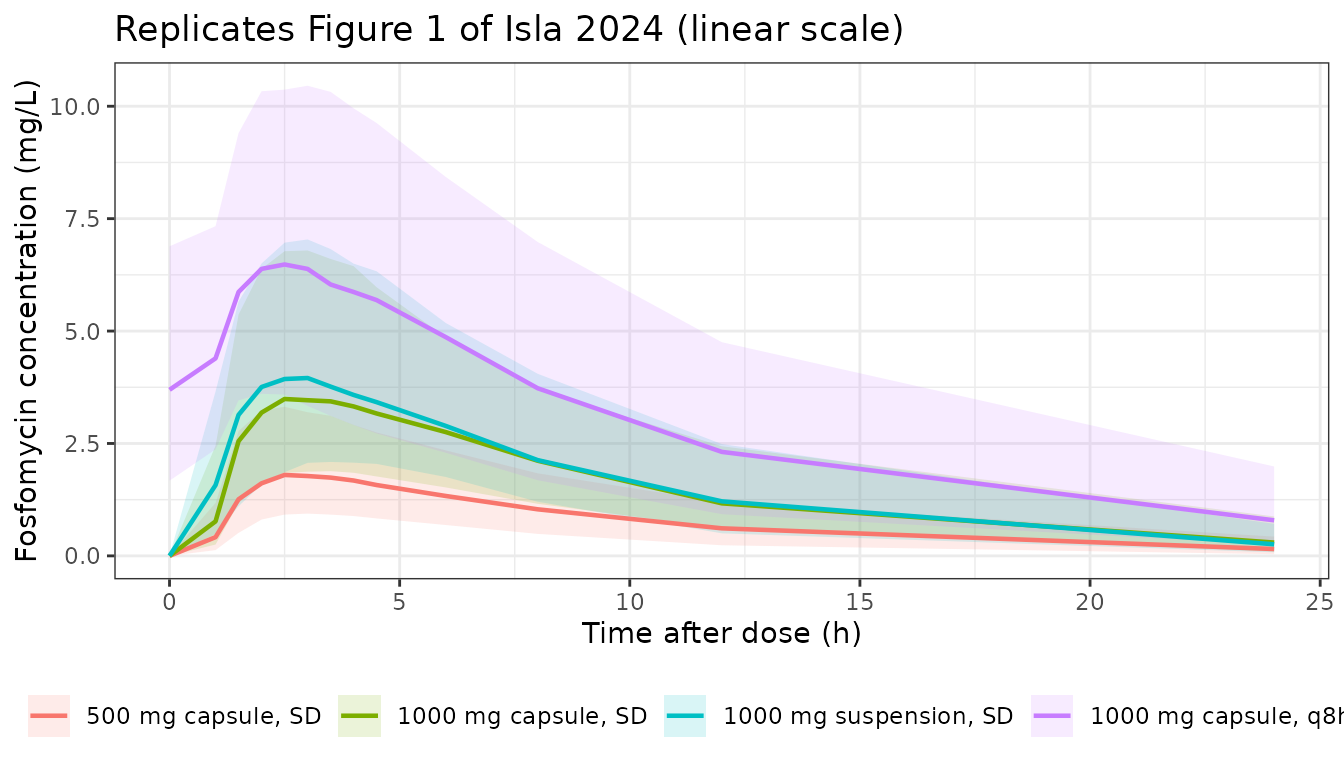

ggplot(dplyr::filter(prof, nca_time > 0, med > 0),
       aes(nca_time, med, colour = treatment)) +
  geom_line(linewidth = 0.8) +
  scale_y_log10() +
  labs(
    x = "Time after dose (h)", y = "Fosfomycin concentration (mg/L)",
    colour = NULL,
    title = "Replicates the log-scale inset of Figure 1 of Isla 2024"
  ) +
  theme_bw() +
  theme(legend.position = "bottom")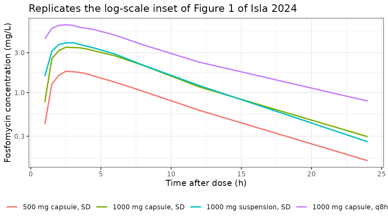

The lag before any measurable concentration (0.84 h for the capsule, 0.71 h for the suspension) and the slow, absorption-limited decline out to 24 h are both visible, as they are in the published figure.

PKNCA validation

sim_nca <- sim |>
  dplyr::filter(!is.na(Cc)) |>
  dplyr::transmute(id, treatment, time = nca_time, Cc)

# Defensive time-zero row (extravascular: pre-dose Cc = 0). Existing time-zero
# rows win because .keep_all keeps the first occurrence after the arrange.
sim_nca <- dplyr::bind_rows(
  sim_nca,
  sim_nca |> dplyr::distinct(id, treatment) |> dplyr::mutate(time = 0, Cc = 0)
) |>
  dplyr::arrange(id, treatment, time) |>
  dplyr::distinct(id, treatment, time, .keep_all = TRUE)

dose_df <- events |>
  dplyr::filter(evid == 1L) |>
  dplyr::transmute(id, treatment, time = nca_time, amt) |>
  # NCA is referenced to the last dose of each arm; earlier maintenance doses
  # sit at negative relative times and are not the NCA dose record.
  dplyr::filter(time == 0)

conc_obj <- PKNCA::PKNCAconc(
  as.data.frame(sim_nca), Cc ~ time | treatment + id,
  concu = "mg/L", timeu = "h"
)
dose_obj <- PKNCA::PKNCAdose(
  as.data.frame(dose_df), amt ~ time | treatment + id,
  doseu = "mg"
)

intervals <- data.frame(
  start      = 0,
  end        = 24,
  cmax       = TRUE,
  tmax       = TRUE,
  auclast    = TRUE,
  aucinf.obs = TRUE,
  half.life  = TRUE
)

nca <- PKNCA::pk.nca(PKNCA::PKNCAdata(conc_obj, dose_obj, intervals = intervals))
#> Warning: Too few points for half-life calculation (min.hl.points=3 with only 2 points)
#> Too few points for half-life calculation (min.hl.points=3 with only 2 points)
#> Too few points for half-life calculation (min.hl.points=3 with only 2 points)
#> Too few points for half-life calculation (min.hl.points=3 with only 2 points)

nca_tbl <- as.data.frame(nca$result) |>
  dplyr::filter(PPTESTCD %in% c("cmax", "tmax", "auclast", "aucinf.obs", "half.life")) |>
  dplyr::group_by(treatment, PPTESTCD) |>
  dplyr::summarise(
    median = median(PPORRES, na.rm = TRUE),
    p05    = quantile(PPORRES, 0.05, na.rm = TRUE),
    p95    = quantile(PPORRES, 0.95, na.rm = TRUE),
    .groups = "drop"
  ) |>
  dplyr::mutate(
    Parameter = nlmixr2lib::ncaParamLabel(PPTESTCD),
    treatment = factor(treatment, levels = arms$treatment)
  ) |>
  dplyr::arrange(treatment, PPTESTCD)

knitr::kable(
  nca_tbl |>
    dplyr::select(Treatment = treatment, Parameter, median, p05, p95) |>
    dplyr::rename("Median" = median, "5th pct" = p05, "95th pct" = p95),
  digits = 2,
  caption = "Simulated non-compartmental parameters by treatment arm (PKNCA; units mg/L, h, mg*h/L)."
)

Simulated non-compartmental parameters by treatment arm (PKNCA; units mg/L, h, mg*h/L).
Treatment	Parameter	Median	5th pct	95th pct
500 mg capsule, SD	AUC0-∞ (obs)	19.39	9.72	35.02
500 mg capsule, SD	AUClast	17.96	9.49	31.44
500 mg capsule, SD	Cmax	1.89	1.05	3.42
500 mg capsule, SD	t½	5.64	3.78	9.19
500 mg capsule, SD	Tmax	3.00	2.00	6.00
1000 mg capsule, SD	AUC0-∞ (obs)	37.88	23.07	67.14
1000 mg capsule, SD	AUClast	35.39	21.36	60.70
1000 mg capsule, SD	Cmax	3.81	2.03	7.19
1000 mg capsule, SD	t½	5.57	3.77	8.99
1000 mg capsule, SD	Tmax	3.00	2.00	4.50
1000 mg suspension, SD	AUC0-∞ (obs)	39.39	24.06	68.07
1000 mg suspension, SD	AUClast	36.71	22.81	62.95
1000 mg suspension, SD	Cmax	4.28	2.10	7.23
1000 mg suspension, SD	t½	5.04	3.58	7.92
1000 mg suspension, SD	Tmax	3.00	1.72	4.50
1000 mg capsule, q8h x 3 d	AUC0-∞ (obs)	78.97	37.59	153.87
1000 mg capsule, q8h x 3 d	AUClast	69.95	35.01	128.33
1000 mg capsule, q8h x 3 d	Cmax	6.63	3.77	10.67
1000 mg capsule, q8h x 3 d	t½	7.17	5.09	10.75
1000 mg capsule, q8h x 3 d	Tmax	2.50	1.50	3.50

Comparison against the published observed values

Isla 2024 does not report point NCA estimates. What the Results section gives is the observed range of Cmax in each arm and a pooled observed range for Tmax:

Cmax ranged from 1.1 to 5.2 mg/L with 500 mg capsules, from 1.2 to 7.0 mg/L with 1000 mg capsules, from 2.5 to 9.5 mg/L with 1000 mg suspension and from 4.3 to 12.3 mg/L with the multiple-dose regimen (1000 mg q8h, 3 days). Regardless of the group, the time to reach Cmax (tmax) ranged from 1 to 4.5 h.

nlmixr2lib::ncaComparisonTable() is not used here because it compares against a reference point estimate, and inventing one from a min-max range (its midpoint, say) would put a number in the table that the paper never reported. The comparison below keeps the published quantity in its published form and asks the question that a range can actually answer: does the simulated central tendency fall inside the observed interval?

published <- tibble::tribble(
  ~treatment,                   ~cmax_lo, ~cmax_hi,
  "500 mg capsule, SD",              1.1,      5.2,
  "1000 mg capsule, SD",             1.2,      7.0,
  "1000 mg suspension, SD",          2.5,      9.5,
  "1000 mg capsule, q8h x 3 d",      4.3,     12.3
)

cmax_cmp <- nca_tbl |>
  dplyr::filter(PPTESTCD == "cmax") |>
  dplyr::select(treatment, sim_median = median, sim_p05 = p05, sim_p95 = p95) |>
  dplyr::left_join(published, by = "treatment") |>
  dplyr::mutate(
    inside = sim_median >= cmax_lo & sim_median <= cmax_hi,
    `Observed range (mg/L)` = sprintf("%.1f - %.1f", cmax_lo, cmax_hi),
    `Simulated median [5th-95th] (mg/L)` =
      sprintf("%.2f [%.2f - %.2f]", sim_median, sim_p05, sim_p95),
    `Median inside observed range` = ifelse(inside, "yes", "NO")
  )

knitr::kable(
  cmax_cmp |>
    dplyr::select(Treatment = treatment, `Observed range (mg/L)`,
                  `Simulated median [5th-95th] (mg/L)`,
                  `Median inside observed range`),
  caption = "Simulated Cmax against the observed Cmax ranges quoted in the Isla 2024 Results."
)

Simulated Cmax against the observed Cmax ranges quoted in the Isla 2024 Results.
Treatment	Observed range (mg/L)	Simulated median [5th-95th] (mg/L)	Median inside observed range
500 mg capsule, SD	1.1 - 5.2	1.89 [1.05 - 3.42]	yes
1000 mg capsule, SD	1.2 - 7.0	3.81 [2.03 - 7.19]	yes
1000 mg suspension, SD	2.5 - 9.5	4.28 [2.10 - 7.23]	yes
1000 mg capsule, q8h x 3 d	4.3 - 12.3	6.63 [3.77 - 10.67]	yes


tmax_med <- nca_tbl |>
  dplyr::filter(PPTESTCD == "tmax") |>
  dplyr::pull(median)

stopifnot(
  # Every arm's simulated median Cmax lands inside the arm's own observed
  # range. These are absolute bounds the paper states, not a bound taken from
  # one run, and the ranges are wide enough that a mis-transcribed dose,
  # volume or clearance -- which move Cmax by tens of percent -- still breaks
  # this. The gate is guarded so it cannot pass vacuously on zero rows.
  nrow(cmax_cmp) == 4L,
  !anyNA(cmax_cmp$cmax_lo),
  all(cmax_cmp$inside),
  # Pooled observed Tmax range, 1 to 4.5 h.
  length(tmax_med) == 4L,
  all(tmax_med >= 1), all(tmax_med <= 4.5)
)

All four arms land inside the published Cmax intervals and all four median Tmax values sit inside the published 1-4.5 h window.

AUC identity

For an extravascular model with apparent clearance, AUC(0-inf) after a single dose must equal Dose / (CL/F) exactly. Both sides here use the same drawn parameters, so the only discrepancy is trapezoidal error on the sampling grid – this is the one place where a tight bound is the right assertion rather than a robust quantile.

dense <- rxode2::et(amt = 1000, cmt = "depot") |>
  rxode2::et(seq(0, 240, by = 0.05), cmt = "central")
ref <- solve_typical(0, ev = dense)
#> ℹ parameter labels from comments will be replaced by 'label()'
#> Warning: some etas defaulted to non-mu referenced, possible parsing error: etaiov_cl_1, etaiov_cl_2, etaiov_cl_3, etaiov_cl_4, etaiov_vc_1, etaiov_vc_2, etaiov_vc_3, etaiov_vc_4
#> as a work-around try putting the mu-referenced expression on a simple line
#> Warning: some etas defaulted to non-mu referenced, possible parsing error: etaiov_cl_1, etaiov_cl_2, etaiov_cl_3, etaiov_cl_4, etaiov_vc_1, etaiov_vc_2, etaiov_vc_3, etaiov_vc_4
#> as a work-around try putting the mu-referenced expression on a simple line

auc_num <- sum(diff(ref$time) * (head(ref$Cc, -1) + tail(ref$Cc, -1)) / 2)
auc_thy <- 1000 / ref$cl[1]

c(numeric = auc_num, `Dose/CL` = auc_thy,
  `% diff` = 100 * (auc_num - auc_thy) / auc_thy)
#>    numeric    Dose/CL     % diff 
#> 42.1853225 42.1940928 -0.0207857

stopifnot(abs(auc_num - auc_thy) / auc_thy < 0.005)

Accumulation on the q8h regimen

The multiple-dose arm is the one place the flip-flop absorption shows up as a clinically visible effect: with an apparent terminal half-life governed by ka = 0.15 1/h rather than by elimination, an 8-hourly regimen accumulates.

auc_by_arm <- nca_tbl |>
  dplyr::filter(PPTESTCD == "auclast") |>
  dplyr::select(treatment, median)

acc <- auc_by_arm$median[auc_by_arm$treatment == "1000 mg capsule, q8h x 3 d"] /
  auc_by_arm$median[auc_by_arm$treatment == "1000 mg capsule, SD"]

# Median AUC(0-24) at steady state over median AUC(0-24) after a single dose.
c(`accumulation ratio (AUC0-24 ss / AUC0-24 sd)` = acc)
#> accumulation ratio (AUC0-24 ss / AUC0-24 sd) 
#>                                     1.976501

# Three q8h doses fall inside a 24 h window, so the ratio must sit meaningfully
# above 1 and below 3; anything outside that would mean the dosing interval or
# the absorption rate was mis-transcribed.
stopifnot(acc > 1.5, acc < 3)

Under flip-flop absorption the trough never returns to zero within the dosing interval, so the multiple-dose profile is best read from ctrough at the end of the interval rather than from a within-interval minimum.

Assumptions and deviations

Erratum in the source. Isla 2024 Table 3 prints a median CL/F of 40.5 L/h at CLCR 150 mL/min. The correct value is 30.5 L/h. Three independent lines of evidence in the paper itself establish this: (i) the covariate model printed in Table 2, CL/F = 23.7 * exp(0.0060 * (CLCR - 108)), gives 30.49 at CLCR = 150; (ii) the mean reported in the very same Table 3 cell, 32.8 L/h, is the log-normal mean of a 30.5 median under the paper’s own IIV and IOV variances (30.5 * 1.0711 = 32.7) and is irreconcilable with a 40.5 median (which would imply 43.4); and (iii) the Discussion states the CL/F increase from CLCR 80 to CLCR 150 is “more than 50%”, which 30.5 / 20.0 = 1.52 satisfies and 40.5 / 20.0 = 2.02 does not. The packaged model implements the Table 2 equation; the 40.5 cell is not reproduced and is excluded from the Table 3 gate above, which is otherwise satisfied by every remaining cell.

Proportional residual error units. Table 2 heads the row “RE proportional (%)” but prints the value 0.199 with a bootstrap 95% CI of 0.159-0.229. The value is the NONMEM proportional-error fraction, i.e. 19.9% CV, not 0.199%; the “(%)” in the header is a table artefact. A 0.199% proportional error would be irreconcilable with the 0.209 mg/L additive term acting on 1-12 mg/L concentrations and with the reported epsilon-shrinkage of 8%. The model encodes propSd <- 0.199.

Peripheral volume parameterisation. The paper does not estimate V2/F directly. Table 2 gives Vss/F = V1 * (1 + theta_V2) with theta_V2 = 4.94, so V2/F is the ratio 4.94 times V1/F. The model encodes lvp <- log(24.4 * 4.94) and applies the same (WT / 64) factor that V1/F carries, which reproduces Vss/F = 144.936 L against the published 144.9 L and the Discussion’s 144.94 L. V2/F is given no random effects of its own: every equation in the Table 2 left-hand column is a typical-value relationship with the etas tabulated separately underneath, so the ratio is read as acting on the typical V1/F rather than on the individual V1/F. If the source NONMEM control stream in fact wrote V2 = V1 * THETA(V2) against the individual V1, V2/F would additionally inherit V1/F’s IIV and IOV. The typical-value predictions – and therefore every check in this vignette – are identical either way; only the spread of the peripheral volume across a simulated cohort would differ. The control stream is not published.

Bioavailability. There was no intravenous arm, so absolute F is not identifiable and all disposition parameters are apparent (CL/F, V1/F, Q/F, V2/F). The model estimates no fdepot term. The paper reports no relative bioavailability between the capsule and the suspension either – the formulation effect is confined to ka and TLAG – so a user simulating the two products should expect the same AUC from both.

Occasion coding. The paper reports IOV on CL/F and V1/F across “study occasions” but does not print the occasion column name, its coding, or the per-occasion estimates. The 1-4 mapping used here (500 mg capsule, 1000 mg capsule, 1000 mg suspension, multiple dose) is this package’s convention; only the number of occasions and the fact that they are the four crossover periods come from the source. One IOV variance per parameter is reported and is shared across occasions, encoded with the registered NONMEM-SAME-equivalent idiom (occasion 1 estimated, occasions 2-4 fixed to it).

Weight exponents. Table 2 writes V1/F = theta_V1 * (BW/64) with no exponent parameter anywhere in the table, so e_wt_vc and e_wt_vp are fixed(1) – making the structurally implicit exponent explicit rather than leaving it inside the equation. There is no body-size term on CL/F or Q/F: the paper’s stepwise search retained weight on V1/F only.

Covariate ranges. Both retained covariates were fitted over a narrow healthy range (CRCL 82.9-158.4 mL/min; weight 51.7-94.8 kg with BMI capped at 30 kg/m^2). The CRCL effect is an uncentred exponential and so extrapolates without bound outside that window. The virtual cohort above truncates derived CRCL to the observed 82.9-158.4 mL/min interval for that reason; the paper’s own Discussion makes the same caution explicit.

Virtual cohort assumptions. Age, weight and serum creatinine are drawn from independent truncated normals matching the Table 1 mean / SD / min / max, and creatinine clearance is then derived with the Cockcroft-Gault equation for women (the estimator Table 1 footnote (a) names) so that renal function and weight are correlated. Individual-level data are not public, so the joint distribution of the three inputs is an assumption; the marginal CRCL distribution that results is checked against the Table 1 mean and median above. The four arms are simulated as independent cohorts rather than as a true crossover, because rxSolve() draws one set of inter-individual random effects per subject ID and re-using an ID across arms would not preserve the pairing. None of the checks in this vignette are paired comparisons, so the difference is presentational.

Sampling grid. The simulated observation grid is the paper’s own 13-point schedule, so simulated Cmax and Tmax are comparable like-for-like with the observed values quoted in the Results. The one exception is the AUC-identity check, which uses a dense grid because it is testing trapezoidal accuracy rather than reproducing an observed quantity.

Non-mu-referencing warning. Building the model emits some etas defaulted to non-mu referenced ... etaiov_cl_1 .... This is inherent to the registered multi-occasion IOV idiom (the same warning is emitted by Blackman_2026_methotrexate.R and the other IOV models in this package) and affects estimation efficiency only, not simulation. All typical-value and cohort checks above are unaffected.