Piperacillin/tazobactam (Wenker 2024)
Source:vignettes/articles/Wenker_2024_piperacillin_tazobactam.Rmd
Wenker_2024_piperacillin_tazobactam.RmdModel and source
- Citation: Wenker SAM, Alabdulkarim N, Readman JB, Slob EMA, Satta G, Ali S, Gadher N, Shulman R, Standing JF. (2024). Defining the pharmacokinetic/pharmacodynamic index of piperacillin/tazobactam within a hollow-fibre infection model to determine target attainment in intensive care patients. JAC-Antimicrobial Resistance 6(2):dlae036. doi:10.1093/jacamr/dlae036. Structural model and all four parameter estimates: main-text Figure 1 (panel annotation). HFIM system design (half-life, circulating volumes, dilution rates, dose levels): Supplementary data, Supplementary Methods.
- Description: In vitro (hollow-fibre infection model, HFIM; six Gram-negative strains). Sigmoidal Emax PK/PD-index model for piperacillin/tazobactam in its clinical 8:1 ratio. Wenker 2024 ran a 21-experiment dose-fractionation study (7 growth controls plus 14 treated arms) in an HFIM and fit, by non-linear least squares on the 24 h timepoint, the change in bacterial density over 24 h as a function of each candidate PK/PD index. fT>MIC (the percentage of the dosing interval during which the free piperacillin/tazobactam concentration exceeds the isolate MIC) was the best-fitting index (AIC 94.1, R^2 0.691) versus fCmax/MIC (AIC 102, R^2 0.526) and fAUC/MIC (AIC 96.9, R^2 0.62). The packaged model is the fT>MIC model of Wenker 2024 Figure 1: effect = e0 - emax * FTMIC_TZP^hill / (ec50^hill + FTMIC_TZP^hill), where effect is the change in log10(CFU/mL) accrued over the 24 h experiment (positive = net growth, negative = net kill), e0 = 4.155 (FIXED) is the change in the untreated growth controls, emax = 8.851 (FIXED) is the maximum achievable reduction of that change, ec50 = 51.01 %fT>MIC is the index value giving half-maximal effect (the paper calls it EI50), and hill = 2.11 is the sigmoidicity coefficient (the paper calls it gam). There is NO pharmacokinetic component: exposure enters solely through the externally supplied per-experiment PK/PD index FTMIC_TZP, and the model has no ODE states because Wenker 2024 fit only the 24 h endpoint and never reported the starting inoculum numerically. The corresponding PK/PD targets recovered from these coefficients are 48% fT>MIC for bacteriostasis, 60% fT>MIC for 1 log10 kill and 75% fT>MIC for 2 log10 kill; the paper reports 48%, 60% and 77% respectively (see the vignette Errata for the 2 log10 discrepancy). Neither between-experiment variability nor a residual error magnitude was reported, so no eta parameters are present and addSd is FIXED at 0; the model is intended for typical-value and target-derivation simulation.
- Article: https://doi.org/10.1093/jacamr/dlae036
- Supplement: Supplementary data at JAC-AMR Online (Supplementary Methods, Figures S1 and S2)
Wenker 2024 is a dose-fractionation study run in a hollow-fibre
infection model (HFIM). Its purpose is to decide which
pharmacokinetic/pharmacodynamic index best predicts the antibacterial
effect of piperacillin/tazobactam, and then to read the clinically
relevant target values off that index. The packaged model is the winning
index model: a sigmoidal Emax function of %fT>MIC.
Two things this paper does that are not packaged here:
- The
fCmax/MICandfAUC/MICindex models. Wenker 2024 reports only their AIC and R^2 (102 / 0.526 and 96.9 / 0.62 respectively, Results) and publishes no coefficients for them, so they are not reconstructable. - The nine-patient ICU target-attainment case series (Table 1). That
analysis simulated plasma concentrations from the primary PK parameters
of a separate publication (Lonsdale 2020, the ABDose study, doi:10.1093/jac/dkaa363)
plus a dialysis clearance parameter borrowed from an ertapenem model
(Eyler 2014, doi:10.1128/AAC.02090-12,
packaged separately as
Eyler_2014_ertapenem). Wenker 2024 reproduces no parameter values from either source, so no PK layer is extractable from this paper. Its Table 1 is used below only as an external consistency check.
Population
The model was fit to 21 HFIM experiments: 7 untreated growth controls and 14 dose-fractionation arms (Methods, “Method for dose-fractionation assays”). Six Gram-negative strains were challenged, one laboratory reference strain (Escherichia coli ATCC 25922) and five clinical isolates. Piperacillin/tazobactam MICs by CLSI broth microdilution were 2, 32, 256, 32, 64 and 4 mg/L for ATCC 25922, DWEC107 (E. coli), DWKC01, JRKC01 (Klebsiella pneumoniae), SWPC02 and SWPC04 (Pseudomonas aeruginosa) respectively (Results, “Dose-fractionation study”).
The HFIM system itself is specified in the Supplementary Methods:
cartridges primed 24 h with PBS then 24 h with Mueller-Hinton broth;
pumps set to mimic a piperacillin half-life of 2 h; cartridge volume 28
mL, tubing 39 mL, central reservoir 10 mL (run 1) or 30 mL (run 2),
giving a total circulating volume of 77 mL or 97 mL and a dilution rate
of 26.6 mL/h or 33.6 mL/h. Drug was infused every 6 h over 24 h, over
either 30 min or 3 h, always in the clinical 8:1 piperacillin:tazobactam
ratio. Dose levels were set from the predicted bolus Cmax: high 128/16
mg/L, middle 32/8 mg/L, low 8/1 mg/L. The circulating medium is
protein-free, so the free fraction is 1 and %fT>MIC
equals %T>MIC in this system.
The same information is available programmatically via the model’s
population metadata
(readModelDb("Wenker_2024_piperacillin_tazobactam")()$population).
Source trace
The per-parameter origin is recorded as an in-file comment next to
each ini() entry in
inst/modeldb/specificDrugs/Wenker_2024_piperacillin_tazobactam.R.
The table below collects them in one place.
| Equation / parameter | Value | Source location |
|---|---|---|
effect <- e0 - emax * FTMIC_TZP^hill / (ec50^hill + FTMIC_TZP^hill) |
n/a | Figure 1 (the plotted fT>MIC model); the parametric form is implied by the panel annotation naming E0, EI50, Emax and gam |
le0 (E0) |
log(4.155), fixed |
Figure 1 panel annotation: E0 = 4.155 FIX
|
lemax (Emax) |
log(8.851), fixed |
Figure 1 panel annotation: Emax = 8.851 FIX
|
lec50 (EI50) |
log(51.01) |
Figure 1 panel annotation: EI50 = 51.01
|
lhill (gam) |
log(2.11) |
Figure 1 panel annotation: gam = 2.11
|
addSd |
fixed(0) |
Not reported. Results reports only AIC = 94.1 and R^2 = 0.691 for the fT>MIC fit |
FTMIC_TZP covariate scale |
percent, 0-100 | Figure 1 x-axis, “Percent of time > MIC” |
| Model-selection statistics | AIC 94.1, R^2 0.68 / 0.691 | Figure 1 panel annotation (0.68) and Results, “Dose-fractionation study” (0.691) |
| Published PK/PD targets | 48 / 60 / 77 %fT>MIC | Results, “Dose-fractionation study” |
| Strain MICs | 2 / 32 / 256 / 32 / 64 / 4 mg/L | Results, “Dose-fractionation study” |
| HFIM half-life, volumes, dilution rates | 2 h; 77 or 97 mL; 26.6 or 33.6 mL/h | Supplementary Methods, “HFIM setup” |
| Dose levels (bolus-equivalent Cmax) | 128/16, 32/8, 8/1 mg/L | Supplementary Methods, “Materials for dose fractionation assay” |
The four ini() values are printed inside the Figure 1
panel, which is a raster image; they are not recoverable by text
extraction from the PDF and were read off the figure at magnification.
See “Assumptions and deviations” below.
Virtual cohort
There is no virtual population here: the model has no between-subject variability and no residual error (see Errata), and the experimental unit is an HFIM cartridge, not a subject. The cohort is instead the experimental design grid the paper actually ran, reconstructed from the Supplementary Methods.
mics <- tibble::tribble(
  ~strain,      ~organism,                 ~mic,
  "ATCC 25922", "E. coli",                    2,
  "DWEC107",    "E. coli",                   32,
  "DWKC01",     "K. pneumoniae",            256,
  "JRKC01",     "K. pneumoniae",             32,
  "SWPC02",     "P. aeruginosa",             64,
  "SWPC04",     "P. aeruginosa",              4
)

# HFIM system settings, Supplementary Methods "HFIM setup". Volumes in L and
# clearances in L/h so concentrations come out in mg/L.
hfim_runs <- tibble::tribble(
  ~run,     ~V,      ~CL,
  "run 1",  0.077,   0.0266,
  "run 2",  0.097,   0.0336
)

# Dose levels, Supplementary Methods: set from the predicted bolus Cmax of
# piperacillin (the tazobactam partner is fixed at 1/8 of these).
dose_levels <- tibble::tribble(
  ~dose_level, ~cmax_target,
  "high",              128,
  "middle",             32,
  "low",                 8
)

# Infusion durations, Methods: "Infusion times were 30 min or 3 h."
infusions <- tibble::tribble(
  ~infusion, ~dur,
  "30 min",     0.5,
  "3 h",        3.0
)

arms <- tidyr::crossing(hfim_runs, dose_levels, infusions) |>
  dplyr::mutate(
    amt       = cmax_target * V,
    treatment = paste(dose_level, infusion)
  )

knitr::kable(
  arms |>
    dplyr::filter(run == "run 1") |>
    dplyr::select(run, dose_level, infusion, V, CL, cmax_target, amt) |>
    dplyr::rename(
      "HFIM run"                    = run,
      "Dose level"                  = dose_level,
      "Infusion"                    = infusion,
      "Circulating volume (L)"      = V,
      "Dilution rate (L/h)"         = CL,
      "Target bolus Cmax (mg/L)"    = cmax_target,
      "Dose amount (mg piperacillin)" = amt
    ),
  digits = 4,
  caption = "HFIM dose-fractionation design grid reconstructed from the Wenker 2024 Supplementary Methods (run 1 configuration shown; run 2 differs only in reservoir size and is checked below)."
)| HFIM run | Dose level | Infusion | Circulating volume (L) | Dilution rate (L/h) | Target bolus Cmax (mg/L) | Dose amount (mg piperacillin) |
|---|---|---|---|---|---|---|
| run 1 | high | 3 h | 0.077 | 0.0266 | 128 | 9.856 |
| run 1 | high | 30 min | 0.077 | 0.0266 | 128 | 9.856 |
| run 1 | low | 3 h | 0.077 | 0.0266 | 8 | 0.616 |
| run 1 | low | 30 min | 0.077 | 0.0266 | 8 | 0.616 |
| run 1 | middle | 3 h | 0.077 | 0.0266 | 32 | 2.464 |
| run 1 | middle | 30 min | 0.077 | 0.0266 | 32 | 2.464 |
Simulation
Step 1 - reconstruct the HFIM exposure
The paper reports no structural PK model for the HFIM (the
Supplementary Methods say only that “a model with the most accurate
pharmacokinetic parameters was selected”, shown graphically in Figure
S2, with no parameter values printed). The system is nonetheless fully
specified by its design: a well-stirred circulating volume emptied at a
fixed dilution rate is a one-compartment model with CL/V
set by the pump. That is what is built here, purely to generate the
%fT>MIC index that the packaged model consumes.
hfim_pk <- rxode2::rxode2({
  d/dt(central) <- -(CL / V) * central
  Cc <- central / V
})

# Dense grid so the time-above-MIC fraction is accurate to ~0.01 percentage points.
obs_grid <- seq(0, 30, by = 0.002)

simulate_arm <- function(V, CL, amt, dur, times) {
  ev <- rxode2::et(amt = amt, dur = dur, ii = 6, until = 23.9, cmt = "central")
  ev <- rxode2::et(ev, times)
  rxode2::rxSolve(hfim_pk, ev, params = c(CL = CL, V = V),
                  returnType = "data.frame")
}

hfim_conc <- do.call(rbind, lapply(seq_len(nrow(arms)), function(i) {
  a <- arms[i, ]
  sim <- simulate_arm(a$V, a$CL, a$amt, a$dur, obs_grid)
  data.frame(
    run        = a$run,
    dose_level = a$dose_level,
    infusion   = a$infusion,
    treatment  = a$treatment,
    time       = sim$time,
    Cc         = sim$Cc,
    stringsAsFactors = FALSE
  )
})) |>
  dplyr::filter(!is.na(Cc))

# The experiment itself ran 0-24 h; the grid is extended to 30 h only so the
# terminal phase after the final dose is available for the half-life check.
ggplot(
  hfim_conc |> dplyr::filter(run == "run 1", time <= 24),
  aes(time, Cc, colour = dose_level, linetype = infusion)
) +
  geom_line() +
  geom_hline(data = mics, aes(yintercept = mic), linewidth = 0.2, alpha = 0.5) +
  scale_y_log10() +
  labs(
    x = "Time (h)", y = "Piperacillin concentration (mg/L)",
    colour = "Dose level", linetype = "Infusion",
    title = "Reconstructed HFIM exposure, q6h over 24 h",
    caption = "Horizontal lines mark the six strain MICs (2, 4, 32, 32, 64, 256 mg/L)."
  )
#> Warning in scale_y_log10(): log-10 transformation introduced infinite values.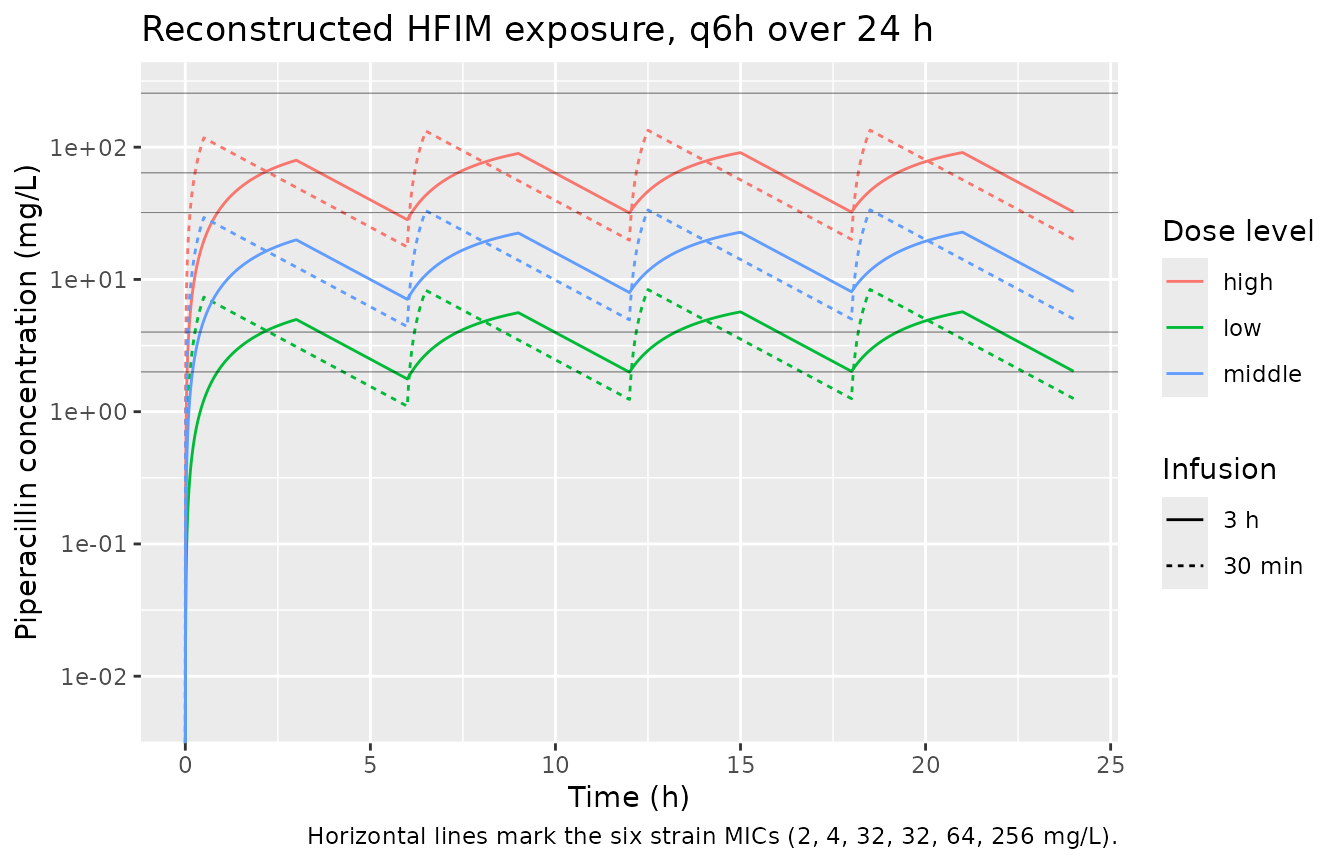
Step 2 - PKNCA validation of the reconstruction
Before the reconstruction is used to drive the PD model, it is checked against the two exposure quantities the paper does state numerically: the design bolus Cmax per dose level, and the 2 h half-life the pumps were set to mimic. A single bolus dose is used here because that is the scenario the dose levels were defined against (“determined based on predicted Cmax concentrations in a bolus scenario”, Supplementary Methods).
bolus_arms <- arms |>
  dplyr::filter(run == "run 1") |>
  dplyr::distinct(dose_level, V, CL, amt, cmax_target) |>
  dplyr::mutate(id = dplyr::row_number(), treatment = dose_level)

bolus_conc <- do.call(rbind, lapply(seq_len(nrow(bolus_arms)), function(i) {
  a  <- bolus_arms[i, ]
  ev <- rxode2::et(amt = a$amt, cmt = "central")
  ev <- rxode2::et(ev, seq(0, 24, by = 0.05))
  sim <- rxode2::rxSolve(hfim_pk, ev, params = c(CL = a$CL, V = a$V),
                         returnType = "data.frame")
  data.frame(
    id = a$id, treatment = a$treatment, time = sim$time, Cc = sim$Cc,
    stringsAsFactors = FALSE
  )
}))

sim_nca <- bolus_conc |>
  dplyr::filter(!is.na(Cc)) |>
  dplyr::select(id, time, Cc, treatment)

# Guarantee a time = 0 row per (id, treatment) so PKNCA can anchor AUC from 0.
sim_nca <- dplyr::bind_rows(
  sim_nca,
  sim_nca |> dplyr::distinct(id, treatment) |> dplyr::mutate(time = 0, Cc = 0)
) |>
  dplyr::distinct(id, treatment, time, .keep_all = TRUE) |>
  dplyr::arrange(id, treatment, time)

conc_obj <- PKNCA::PKNCAconc(sim_nca, Cc ~ time | treatment + id)

dose_df <- bolus_arms |> dplyr::mutate(time = 0) |> dplyr::select(id, time, amt, treatment)
dose_obj <- PKNCA::PKNCAdose(dose_df, amt ~ time | treatment + id)

intervals <- data.frame(
  start      = 0,
  end        = Inf,
  cmax       = TRUE,
  tmax       = TRUE,
  aucinf.obs = TRUE,
  half.life  = TRUE
)

nca_res <- PKNCA::pk.nca(PKNCA::PKNCAdata(conc_obj, dose_obj, intervals = intervals))
Comparison against the published HFIM design
published <- tibble::tribble(
  ~treatment, ~cmax, ~half.life,
  "high",       128,        2.0,
  "middle",      32,        2.0,
  "low",          8,        2.0
)

cmp <- nlmixr2lib::ncaComparisonTable(
  simulated     = nca_res,
  reference     = published,
  by            = "treatment",
  params        = c("cmax", "half.life"),
  units         = c(cmax = "mg/L", half.life = "h"),
  tolerance_pct = 20
)

knitr::kable(
  cmp,
  caption = paste(
    "Reconstructed HFIM exposure vs. the design values stated in the Wenker 2024",
    "Supplementary Methods (bolus-equivalent Cmax per dose level; pump half-life).",
    "* differs from reference by >20%."
  ),
  align = c("l", "l", "r", "r", "r")
)| NCA parameter | treatment | Reference | Simulated | % diff |
|---|---|---|---|---|
| Cmax (mg/L) | high | 128 | 128 | +0.0% |
| Cmax (mg/L) | middle | 32 | 32 | +0.0% |
| Cmax (mg/L) | low | 8 | 8 | +0.0% |
| t½ (h) | high | 2 | 2.01 | +0.3% |
| t½ (h) | middle | 2 | 2.01 | +0.3% |
| t½ (h) | low | 2 | 2.01 | +0.3% |
Every row agrees with the stated design, which confirms that the
reconstructed CL and V reproduce the paper’s
HFIM system rather than merely resembling it.
Step 3 - derive the PK/PD index per experiment
%fT>MIC is the percentage of the 24 h experiment
during which the concentration exceeds the strain’s MIC. The drug pump
was started at inoculation (Figure S1 caption), so the whole 24 h window
is on drug.
ftmic <- hfim_conc |>
  dplyr::filter(time <= 24) |>
  tidyr::crossing(mics) |>
  dplyr::group_by(run, dose_level, infusion, treatment, strain, organism, mic) |>
  dplyr::summarise(FTMIC_TZP = 100 * mean(Cc > mic), .groups = "drop")

# The two HFIM run configurations were tuned to the same 2 h half-life, so the
# index they produce should be all but identical. Confirm rather than assume.
run_gap <- ftmic |>
  tidyr::pivot_wider(
    id_cols = c(dose_level, infusion, strain), names_from = run, values_from = FTMIC_TZP
  ) |>
  dplyr::mutate(gap = abs(`run 1` - `run 2`))
stopifnot(max(run_gap$gap) < 1)

knitr::kable(
  ftmic |>
    dplyr::filter(run == "run 1") |>
    tidyr::pivot_wider(
      id_cols = c(dose_level, infusion), names_from = strain, values_from = FTMIC_TZP
    ) |>
    dplyr::rename("Dose level" = dose_level, "Infusion" = infusion),
  digits = 1,
  caption = paste(
    "Percent fT>MIC per design arm and strain (run 1). Largest run 1 vs run 2",
    "discrepancy:", sprintf("%.2f", max(run_gap$gap)), "percentage points."
  )
)| Dose level | Infusion | ATCC 25922 | DWEC107 | DWKC01 | JRKC01 | SWPC02 | SWPC04 |
|---|---|---|---|---|---|---|---|
| high | 3 h | 99.8 | 94.3 | 0 | 94.3 | 40.4 | 99.6 |
| high | 30 min | 100.0 | 74.6 | 0 | 74.6 | 38.9 | 99.9 |
| low | 3 h | 94.3 | 0.0 | 0 | 0.0 | 0.0 | 40.4 |
| low | 30 min | 74.6 | 0.0 | 0 | 0.0 | 0.0 | 38.9 |
| middle | 3 h | 99.2 | 0.0 | 0 | 0.0 | 0.0 | 98.3 |
| middle | 30 min | 99.9 | 1.9 | 0 | 1.9 | 0.0 | 99.7 |
DWKC01 (MIC 256 mg/L) is never covered at any dose
level, giving %fT>MIC = 0 and therefore uninhibited
growth. That reproduces the cluster of treated points sitting at the
left-hand edge of Wenker 2024 Figure 1 alongside the growth
controls.
Step 4 - predict the 24 h change in bacterial density
mod <- readModelDb("Wenker_2024_piperacillin_tazobactam")

design_events <- ftmic |>
  dplyr::filter(run == "run 1") |>
  dplyr::mutate(id = dplyr::row_number(), time = 0, evid = 0, amt = NA_real_)

design_pred <- rxode2::rxSolve(
  mod, events = design_events,
  keep = c("dose_level", "infusion", "strain", "organism", "mic")
) |>
  as.data.frame()
#> Warning: multi-subject simulation without without 'omega'

knitr::kable(
  design_pred |>
    dplyr::select(dose_level, infusion, strain, organism, FTMIC_TZP, effect) |>
    dplyr::arrange(dplyr::desc(FTMIC_TZP)) |>
    head(12) |>
    dplyr::rename(
      "Dose level"                       = dose_level,
      "Infusion"                         = infusion,
      "Strain"                           = strain,
      "Organism"                         = organism,
      "%fT>MIC"                          = FTMIC_TZP,
      "Predicted 24 h change (log10 CFU/mL)" = effect
    ),
  digits = 2,
  caption = "Packaged model applied to the reconstructed design grid (12 highest-exposure arms)."
)| Dose level | Infusion | Strain | Organism | %fT>MIC | Predicted 24 h change (log10 CFU/mL) |
|---|---|---|---|---|---|
| high | 30 min | ATCC 25922 | E. coli | 99.97 | -2.97 |
| high | 30 min | SWPC04 | P. aeruginosa | 99.93 | -2.97 |
| middle | 30 min | ATCC 25922 | E. coli | 99.87 | -2.97 |
| high | 3 h | ATCC 25922 | E. coli | 99.80 | -2.97 |
| middle | 30 min | SWPC04 | P. aeruginosa | 99.73 | -2.97 |
| high | 3 h | SWPC04 | P. aeruginosa | 99.60 | -2.96 |
| middle | 3 h | ATCC 25922 | E. coli | 99.19 | -2.95 |
| middle | 3 h | SWPC04 | P. aeruginosa | 98.33 | -2.92 |
| high | 3 h | DWEC107 | E. coli | 94.32 | -2.80 |
| high | 3 h | JRKC01 | K. pneumoniae | 94.32 | -2.80 |
| low | 3 h | ATCC 25922 | E. coli | 94.32 | -2.80 |
| high | 30 min | DWEC107 | E. coli | 74.57 | -1.95 |
Replicate published figures
Figure 1 - the fT>MIC index model
curve_events <- data.frame(
  id        = 1L,
  FTMIC_TZP = seq(0, 100, by = 0.1)
) |>
  dplyr::mutate(time = dplyr::row_number() - 1, evid = 0, amt = NA_real_)

curve <- rxode2::rxSolve(mod, events = curve_events) |> as.data.frame()

targets <- tibble::tibble(
  endpoint  = c("Bacteriostasis", "1 log10 kill", "2 log10 kill"),
  effect    = c(0, -1, -2),
  published = c(48, 60, 77)
) |>
  dplyr::mutate(
    model = vapply(
      effect,
      function(y) {
        stats::uniroot(
          function(x) stats::approx(curve$FTMIC_TZP, curve$effect, xout = x)$y - y,
          interval = c(1, 99)
        )$root
      },
      numeric(1)
    )
  )

ggplot(curve, aes(FTMIC_TZP, effect)) +
  geom_line(linewidth = 0.8) +
  geom_hline(yintercept = 0, linewidth = 0.3) +
  geom_point(
    data = design_pred,
    aes(FTMIC_TZP, effect, colour = dose_level, shape = organism),
    size = 2.4, alpha = 0.85, inherit.aes = FALSE
  ) +
  geom_vline(data = targets, aes(xintercept = model), linetype = "dotted", linewidth = 0.3) +
  scale_x_continuous(limits = c(0, 100)) +
  labs(
    x = "Percent of time > MIC",
    y = "Change in log10 CFU/mL over 24 h",
    colour = "Dose level", shape = "Organism",
    title = "Figure 1 - fT>MIC PK/PD index model for piperacillin/tazobactam",
    caption = paste(
      "Replicates Figure 1 of Wenker 2024. Line: the packaged model.",
      "Points: the packaged model evaluated at the reconstructed design-grid",
      "exposures. Dotted verticals: the model-derived PK/PD targets."
    )
  )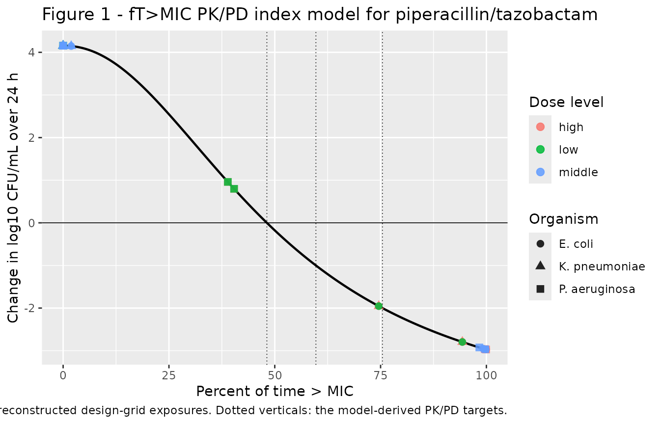
The reconstructed design points land where Wenker 2024 Figure 1 places its experimental points: a cluster at 0% (the uncovered DWKC01 arms, predicted to grow by the full 4.155 log10), an intermediate group in the 39-45% band, and a group at 74-100% where net kill is predicted.
PK/PD targets
targets |>
  dplyr::mutate(`% diff` = 100 * (model - published) / published) |>
  dplyr::select(endpoint, effect, published, model, `% diff`) |>
  dplyr::rename(
    "Endpoint"                        = endpoint,
    "Change in log10 CFU/mL"          = effect,
    "Published target (%fT>MIC)"      = published,
    "Model-derived target (%fT>MIC)"  = model
  ) |>
  knitr::kable(
    digits = 2,
    caption = "PK/PD targets recovered from the packaged Figure 1 coefficients vs. the values Wenker 2024 reports in Results."
)| Endpoint | Change in log10 CFU/mL | Published target (%fT>MIC) | Model-derived target (%fT>MIC) | % diff |
|---|---|---|---|---|
| Bacteriostasis | 0 | 48 | 48.14 | 0.28 |
| 1 log10 kill | -1 | 60 | 59.72 | -0.46 |
| 2 log10 kill | -2 | 77 | 75.43 | -2.03 |
Bacteriostasis and 1 log10 kill are reproduced to within 0.3 percentage points. The 2 log10 kill target is not: the packaged coefficients give 75.4% where the paper reports 77%. This is an internal inconsistency in the source, not a transcription error - see the Errata below.
External consistency check: the ICU case series
Wenker 2024 Table 1 reports, for each of nine ICU patients, the
median %fT>MIC from a 1000-fold simulation and the
resulting probability of target attainment at each of the three
thresholds. That simulation used a different (unreported) PK model, so
the packaged model cannot reproduce the PTA percentages. It can,
however, be checked for consistency: a patient whose median
%fT>MIC sits above a threshold must have PTA above 50%
at that threshold, and the model’s predicted 24 h change at that median
exposure should be at least as much kill as the corresponding
endpoint.
table1 <- tibble::tribble(
  ~patient, ~organism,        ~regimen, ~ftmic_median, ~pta_stasis, ~pta_1log, ~pta_2log,
  1L, "E. coli",       "q8h", 100,  99.5, 99.5, 97.0,
  2L, "P. aeruginosa", "q6h",  92,  94.0, 88.0, 85.0,
  3L, "E. coli",       "q6h",  80,  91.0, 79.0, 54.0,
  4L, "E. coli",       "q6h", 100,  97.0, 93.0, 84.0,
  5L, "K. pneumoniae", "q8h",  90,  93.0, 83.0, 66.0,
  6L, "E. coli",       "q8h", 100, 100.0, 100.0, 100.0,
  7L, "E. coli",       "q8h",  58,  68.0, 47.0, 28.0,
  8L, "E. coli",       "q6h", 100,  99.5, 98.5, 96.0,
  9L, "K. pneumoniae", "q8h", 100,  99.5, 99.5, 97.5
)

patient_events <- table1 |>
  dplyr::transmute(
    id = patient, FTMIC_TZP = ftmic_median,
    time = 0, evid = 0, amt = NA_real_
  )

patient_pred <- rxode2::rxSolve(mod, events = patient_events) |>
  as.data.frame() |>
  dplyr::select(id, FTMIC_TZP, effect) |>
  dplyr::rename(patient = id)
#> Warning: multi-subject simulation without without 'omega'

check <- table1 |>
  dplyr::left_join(patient_pred, by = "patient") |>
  dplyr::mutate(
    above_stasis = ftmic_median >= targets$model[1],
    above_2log   = ftmic_median >= targets$model[3]
  )

# Consistency: median index above a threshold implies PTA > 50% at that threshold.
stopifnot(all(check$pta_stasis[check$above_stasis] > 50))
stopifnot(all(check$pta_2log[check$above_2log] > 50))

check |>
  dplyr::select(patient, organism, regimen, ftmic_median, effect,
                pta_stasis, pta_1log, pta_2log) |>
  dplyr::rename(
    "Patient"                                = patient,
    "Organism"                               = organism,
    "Regimen"                                = regimen,
    "Median %fT>MIC (published)"             = ftmic_median,
    "Model 24 h change (log10 CFU/mL)"       = effect,
    "%PTA stasis"                            = pta_stasis,
    "%PTA 1 log10"                           = pta_1log,
    "%PTA 2 log10"                           = pta_2log
  ) |>
  knitr::kable(
    digits = 2,
    caption = paste(
      "Wenker 2024 Table 1 (published columns) with the packaged model's predicted",
      "24 h change at each patient's published median exposure. The PTA columns come",
      "from the paper's own simulation using an unrelated PK model and are shown for",
      "context, not reproduced here."
    )
)| Patient | Organism | Regimen | Median %fT>MIC (published) | Model 24 h change (log10 CFU/mL) | %PTA stasis | %PTA 1 log10 | %PTA 2 log10 |
|---|---|---|---|---|---|---|---|
| 1 | E. coli | q8h | 100 | -2.97 | 99.5 | 99.5 | 97.0 |
| 2 | P. aeruginosa | q6h | 92 | -2.72 | 94.0 | 88.0 | 85.0 |
| 3 | E. coli | q6h | 80 | -2.23 | 91.0 | 79.0 | 54.0 |
| 4 | E. coli | q6h | 100 | -2.97 | 97.0 | 93.0 | 84.0 |
| 5 | K. pneumoniae | q8h | 90 | -2.64 | 93.0 | 83.0 | 66.0 |
| 6 | E. coli | q8h | 100 | -2.97 | 100.0 | 100.0 | 100.0 |
| 7 | E. coli | q8h | 58 | -0.87 | 68.0 | 47.0 | 28.0 |
| 8 | E. coli | q6h | 100 | -2.97 | 99.5 | 98.5 | 96.0 |
| 9 | K. pneumoniae | q8h | 100 | -2.97 | 99.5 | 99.5 | 97.5 |
Patient 7 is the only one whose median exposure (58% fT>MIC) falls below the 1 log10 kill target; the paper’s own PTA columns agree, giving that patient the lowest attainment of all nine at every threshold.
Assumptions and deviations
All four parameter values are figure-derived.
E0,EI50,Emaxandgamare printed only inside the Wenker 2024 Figure 1 panel, which is a raster image in both the publisher PDF and the EuropePMC deposit. They are not recoverable by text extraction and were read off the figure at 3x magnification (AIC = 94.1,R2 = 0.68,E0 = 4.155 FIX,EI50 = 51.01,Emax = 8.851 FIX,gam = 2.11). No numeric parameter table exists anywhere in the paper or its supplement.The parametric form is inferred from the parameter names plus the plotted curve. Wenker 2024 never writes the equation out; it states only that non-linear least squares were used on the 24 h timepoint. The names
E0,EI50(not EC50),Emaxandgamidentify an inhibitory sigmoidal Emax, andeffect = E0 - Emax * I^gam / (EI50^gam + I^gam)reproduces the plotted curve at its intercept (4.155 at 0%), its shape (2.55 / -0.18 / -1.98 at 25 / 50 / 75%), its value at 100% (-2.97), and two of the three published targets to within 0.3 percentage points. No other single-sigmoid form does.The 2 log10 kill target does not reconcile. The published coefficients give 75.4% fT>MIC for a -2 log10 change; Wenker 2024 Results reports 77%. The 48% and 60% targets reconcile to 48.1% and 59.7%. The three published targets are not simultaneously consistent with any single sigmoid holding
E0 = 4.155andEmax = 8.851: 48 and 60 together implygam = 2.04, while 48 and 77 together implygam = 2.01, and the fitted value is 2.11. The packaged model encodes the printed coefficients, since those are what define the fitted curve; a user wanting the paper’s headline 77% should use it as a rounded-up operating target rather than expect the model to return it.No between-experiment variability and no residual error. Wenker 2024 reports only AIC and R^2 for the fit.
addSdis thereforefixed(0)rather than invented, and no eta parameters are present. The model is for typical-value and target-derivation simulation, not for VPC-style stochastic work. This follows the same convention asWen_2016_enrofloxacin_*andChen_2023_tilmicosin.No ODE state, and no starting inoculum. The source fit a single 24 h endpoint and never reports the inoculum numerically (the Methods say it was read by UV spectrophotometer OD; the resulting trajectories appear only graphically in Figure S1). The packaged model is therefore algebraic and predicts the change in log10 CFU/mL, which is exactly the quantity fit. The alternative encoding used by
Chen_2023_tilmicosin- an ODE on bacterial density with the interval change spread uniformly across the interval - was not used here because it would require an initial condition the paper does not supply.The HFIM PK reconstruction in this vignette is design-derived, not model-derived. Wenker 2024 fit a PK model to its bioassay concentrations in nlmixr2 but publishes no parameters for it (Supplementary Methods; the fit appears only as the Figure S2 goodness-of-fit plot). The one-compartment system built above uses the stated design settings - circulating volume, dilution rate, dosing interval, infusion duration, and target bolus Cmax - and is validated against the two design quantities the paper does state numerically (bolus Cmax per dose level and the 2 h pump half-life). It is scaffolding for generating the index; it is not part of the packaged model and should not be mistaken for a piperacillin popPK model.
Which 24 h window defines
%fT>MICis inferred. The paper defines the index as “the percentage of time the piperacillin/tazobactam concentration was above the MIC” without naming a window. The whole 24 h experiment is used here because the drug pump was started at inoculation (Figure S1 caption) and the experiment ran 24 h. Using only the final q6h interval instead would change the reconstructed values by at most a few percentage points, since the system reaches steady state within two half-lives.Strain-to-arm assignment is not published. Wenker 2024 does not say which dose level, infusion duration or HFIM run configuration was paired with which strain in each of the 14 treated experiments. The design grid above therefore enumerates all combinations rather than reproducing the 14 actual arms, and the points plotted on the Figure 1 replication are model predictions across that grid, not the paper’s observed data.
Free fraction is 1 by construction. The HFIM circulates protein-free Mueller-Hinton broth, so
%fT>MICand%T>MICcoincide in the source experiments. A user applying this model to plasma exposure must supply a free-drug time-above-MIC, not a total-drug one.FTMIC_TZPis a new canonical covariate, registered with this extraction ininst/references/covariate-columns.mdas the first member of theFTMIC_<DRUG>family. It is the parallel canonical anticipated by theAUC_TILMentry’s notes for a time-above-MIC exposure metric.