Guhong injection PK/PD in myocardial ischemia/reperfusion rats (Chen 2024)
Source:vignettes/articles/Chen_2024_guhongInjection.Rmd
Chen_2024_guhongInjection.RmdModel and source
Guhong injection (GHI) is a Chinese herbal compound preparation of N-acetyl-L-glutamine plus an aqueous safflower (Carthamus tinctorius L.) extract, used clinically for cardio- and cerebrovascular disease. Chen 2024 gave a single tail-vein injection of GHI at 2.5, 5 or 10 mL/kg to male Sprague-Dawley rats subjected to myocardial ischemia/reperfusion (MI/R) injury, quantified eight constituents in plasma by LC-MS/MS, and fitted a two-compartment intravenous disposition model to each constituent in each dose group. Four myocardial-injury biomarkers were measured in parallel and linked to the plasma concentrations through direct-effect sigmoid-Emax models.
The paper contributes eight independent model files - one per quantified constituent, because the authors fitted each constituent separately:
guhong_models <- c(
  "Chen_2024_nAcetylglutamine_rat",
  "Chen_2024_hydroxysafflorYellowA_rat",
  "Chen_2024_chlorogenicAcid_rat",
  "Chen_2024_pCoumaricAcid_rat",
  "Chen_2024_rutin_rat",
  "Chen_2024_hyperoside_rat",
  "Chen_2024_kaempferol3ORutinoside_rat",
  "Chen_2024_kaempferol3OGlucoside_rat"
)- Citation: Chen HY, Li C, Shao CY, Wu YJ, Wan HT, He Y (2024). An auxiliary strategy of partial least squares regression in pharmacokinetic/pharmacodynamic studies: A case of application of guhong injection in myocardial ischemia/reperfusion rats. J Food Drug Anal 32(1):79-102. doi:10.38212/2224-6614.3492
- Article: J Food Drug Anal 2024;32(1):79-102
The description of one member, for orientation:
cat(strwrap(readModelDb("Chen_2024_chlorogenicAcid_rat")()$description, 76), sep = "\n")
#> Preclinical (rat). Two-compartment intravenous pharmacokinetic model for
#> chlorogenic acid (CGA), one of eight constituents of guhong injection (GHI)
#> quantified in plasma, in male Sprague-Dawley rats subjected to 30 min
#> left-anterior-descending ligation followed by 1 h reperfusion (myocardial
#> ischemia/reperfusion, MI/R) (Chen 2024). GHI was given as a single
#> tail-vein injection of 2.5, 5 or 10 mL/kg; the chlorogenic acid dose is the
#> GHI volume dose times its content in GHI (12.9 ug/mL), i.e. 32.25 ug/kg,
#> 64.5 ug/kg, 129 ug/kg. Disposition was fitted separately in each dose group
#> with Drug and Statistics (DAS) v3.2.6, so V1, V2, CL1 and Q are selected
#> from the covariate DOSE_GHI_MLKG rather than through a dose-covariate
#> function the authors did not fit. Direct-effect sigmoid-Emax models link
#> the chlorogenic acid plasma concentration to the GHI-minus-model-group
#> difference in creatine kinase-MB (CK-MB), ischemia-modified albumin (IMA),
#> cardiac troponin I (cTn I) and alpha-hydroxybutyrate dehydrogenase
#> (alpha-HBDH) (E = Emax * C^gamma / (ED50^gamma + C^gamma); Tables 12, 13,
#> 14, 15). Chen 2024 fitted a PK/PD model only for the analyte/biomarker/dose
#> combinations whose PLSR coefficient was negative, so the effect of an
#> unfitted combination is returned as zero rather than extrapolated. No
#> between-subject variability or residual error was reported; every parameter
#> is fixed at the published mean and the residual SDs are fixed at zero.
Population
Adult male Sprague-Dawley rats weighing 320-340 g were randomised to six groups (Chen 2024 Sections 2.2-2.3): sham, MI/R model, three GHI dose groups (GHI-L 2.5 mL/kg, GHI-M 5 mL/kg, GHI-H 10 mL/kg) and a verapamil hydrochloride 0.95 mg/kg positive control. MI/R was induced by 30 min of left-anterior- descending coronary artery ligation followed by 1 h of reperfusion. Saline (10 mL/kg) was given to the sham and model groups. Plasma was drawn from the retro-orbital venous plexus at 2, 5, 10, 20, 40, 60, 90, 120, 240 and 360 min. The pharmacokinetic parameters (Tables 2-9) come from n = 6 rats per GHI dose group; the biomarker series (Figure 3) from n = 3 per group. Only male rats were studied, so no sex covariate applies, and no age or race/ethnicity data are reported.
The same information is available programmatically:
str(readModelDb("Chen_2024_chlorogenicAcid_rat")()$population)
#> List of 9
#>  $ species      : chr "rat (Sprague-Dawley)"
#>  $ n_subjects   : num 18
#>  $ n_studies    : num 1
#>  $ sex          : chr "male"
#>  $ weight_range : chr "320-340 g"
#>  $ disease_state: chr "myocardial ischemia/reperfusion injury (30 min LAD ligation, 1 h reperfusion)"
#>  $ dose_range   : chr "guhong injection 2.5, 5 or 10 mL/kg as a single tail-vein injection"
#>  $ regions      : chr "China"
#>  $ notes        : chr "Chen 2024 Sections 2.2-2.4: adult male Sprague-Dawley rats, 320-340 g, randomised to six groups (sham, model, G"| __truncated__
Analytes, content in GHI, and administered dose
Each constituent’s dose is the GHI volume dose multiplied by its
content in the preparation (Chen 2024 Results 3.2). This is what the
DOSE_GHI_MLKG covariate encodes, and it is what turns one
injection into eight simultaneous doses.
analytes <- tibble::tribble(
  ~model,                                 ~analyte,                    ~abbrev, ~content, ~content_units, ~dose_units, ~conc_units, ~pk_table,
  "Chen_2024_nAcetylglutamine_rat",       "N-acetyl-L-glutamine",      "NAG",   30.0,     "mg/mL",        "mg/kg",     "ug/mL",     7L,
  "Chen_2024_hydroxysafflorYellowA_rat",  "hydroxysafflor yellow A",   "HSYA",   1.0,     "mg/mL",        "mg/kg",     "ug/mL",     3L,
  "Chen_2024_chlorogenicAcid_rat",        "chlorogenic acid",          "CGA",   12.9,     "ug/mL",        "ug/kg",     "ng/mL",     2L,
  "Chen_2024_pCoumaricAcid_rat",          "p-coumaric acid",           "pCA",   78.3,     "ug/mL",        "ug/kg",     "ng/mL",     8L,
  "Chen_2024_rutin_rat",                  "rutin",                     "RT",    11.7,     "ug/mL",        "ug/kg",     "ng/mL",     9L,
  "Chen_2024_hyperoside_rat",             "hyperoside",                "HYP",    3.4,     "ug/mL",        "ug/kg",     "ng/mL",     4L,
  "Chen_2024_kaempferol3ORutinoside_rat", "kaempferol-3-O-rutinoside", "K-3-R", 65.7,     "ug/mL",        "ug/kg",     "ng/mL",     6L,
  "Chen_2024_kaempferol3OGlucoside_rat",  "kaempferol-3-O-glucoside",  "K-3-G",  8.7,     "ug/mL",        "ug/kg",     "ng/mL",     5L
)

dose_groups <- tibble::tibble(
  group = factor(c("GHI-L", "GHI-M", "GHI-H"), levels = c("GHI-L", "GHI-M", "GHI-H")),
  ghi_dose = c(2.5, 5, 10)
)

dosing <- tidyr::expand_grid(analytes, dose_groups) |>
  dplyr::mutate(amt = content * ghi_dose)

dosing |>
  dplyr::select(analyte, abbrev, content, content_units, group, ghi_dose, amt, dose_units) |>
  dplyr::rename(
    "Analyte" = analyte, "Abbrev." = abbrev,
    "Content in GHI" = content, "Content units" = content_units,
    "Dose group" = group, "GHI dose (mL/kg)" = ghi_dose,
    "Analyte dose" = amt, "Dose units" = dose_units
  ) |>
knitr::kable(caption = "Analyte dose per GHI dose group (Chen 2024 Results 3.2 and Section 2.3).")| Analyte | Abbrev. | Content in GHI | Content units | Dose group | GHI dose (mL/kg) | Analyte dose | Dose units |
|---|---|---|---|---|---|---|---|
| N-acetyl-L-glutamine | NAG | 30.0 | mg/mL | GHI-L | 2.5 | 75.00 | mg/kg |
| N-acetyl-L-glutamine | NAG | 30.0 | mg/mL | GHI-M | 5.0 | 150.00 | mg/kg |
| N-acetyl-L-glutamine | NAG | 30.0 | mg/mL | GHI-H | 10.0 | 300.00 | mg/kg |
| hydroxysafflor yellow A | HSYA | 1.0 | mg/mL | GHI-L | 2.5 | 2.50 | mg/kg |
| hydroxysafflor yellow A | HSYA | 1.0 | mg/mL | GHI-M | 5.0 | 5.00 | mg/kg |
| hydroxysafflor yellow A | HSYA | 1.0 | mg/mL | GHI-H | 10.0 | 10.00 | mg/kg |
| chlorogenic acid | CGA | 12.9 | ug/mL | GHI-L | 2.5 | 32.25 | ug/kg |
| chlorogenic acid | CGA | 12.9 | ug/mL | GHI-M | 5.0 | 64.50 | ug/kg |
| chlorogenic acid | CGA | 12.9 | ug/mL | GHI-H | 10.0 | 129.00 | ug/kg |
| p-coumaric acid | pCA | 78.3 | ug/mL | GHI-L | 2.5 | 195.75 | ug/kg |
| p-coumaric acid | pCA | 78.3 | ug/mL | GHI-M | 5.0 | 391.50 | ug/kg |
| p-coumaric acid | pCA | 78.3 | ug/mL | GHI-H | 10.0 | 783.00 | ug/kg |
| rutin | RT | 11.7 | ug/mL | GHI-L | 2.5 | 29.25 | ug/kg |
| rutin | RT | 11.7 | ug/mL | GHI-M | 5.0 | 58.50 | ug/kg |
| rutin | RT | 11.7 | ug/mL | GHI-H | 10.0 | 117.00 | ug/kg |
| hyperoside | HYP | 3.4 | ug/mL | GHI-L | 2.5 | 8.50 | ug/kg |
| hyperoside | HYP | 3.4 | ug/mL | GHI-M | 5.0 | 17.00 | ug/kg |
| hyperoside | HYP | 3.4 | ug/mL | GHI-H | 10.0 | 34.00 | ug/kg |
| kaempferol-3-O-rutinoside | K-3-R | 65.7 | ug/mL | GHI-L | 2.5 | 164.25 | ug/kg |
| kaempferol-3-O-rutinoside | K-3-R | 65.7 | ug/mL | GHI-M | 5.0 | 328.50 | ug/kg |
| kaempferol-3-O-rutinoside | K-3-R | 65.7 | ug/mL | GHI-H | 10.0 | 657.00 | ug/kg |
| kaempferol-3-O-glucoside | K-3-G | 8.7 | ug/mL | GHI-L | 2.5 | 21.75 | ug/kg |
| kaempferol-3-O-glucoside | K-3-G | 8.7 | ug/mL | GHI-M | 5.0 | 43.50 | ug/kg |
| kaempferol-3-O-glucoside | K-3-G | 8.7 | ug/mL | GHI-H | 10.0 | 87.00 | ug/kg |
Source trace
Every ini() entry carries an in-file comment naming its
source cell. The table below collects the provenance by kind; the
per-value comments in
inst/modeldb/specificDrugs/Chen_2024_*_rat.R are the
authoritative record.
| Equation / parameter | Source location |
|---|---|
d/dt(central), d/dt(peripheral1)
(two-compartment IV disposition) |
Chen 2024 Section 2.9 (“we first investigated the PK parameters with a two-compartment model”) and formulas 3-12 |
lvc_ghil / lvc_ghim /
lvc_ghih (V1, L/kg) |
Tables 2-9, row V1, columns GHI-L / GHI-M / GHI-H |
lvp_ghil / lvp_ghim /
lvp_ghih (V2, L/kg) |
Tables 2-9, row V2
|
lcl_ghil / lcl_ghim /
lcl_ghih (CL1, L/h/kg) |
Tables 2-9, row CL1
|
lq_ghil / lq_ghim / lq_ghih
(Q, L/h/kg) |
Tables 2-9, row Q (formula 12:
Q = k12 * V1) |
kel <- cl / vc, k12 <- q / vc,
k21 <- q / vp
|
Chen 2024 formulas 5, 6 and 12 (CL = k * V,
Q = k12 * V1) |
E = Emax * C^gamma / (ED50^gamma + C^gamma) |
Chen 2024 Section 3.6, PK/PD equation form |
lemax_ckmb_*, lec50_ckmb_*,
lhill_ckmb_*
|
Table 12 (delta CK-MB), row for the analyte within the dose-group block |
lemax_ima_*, lec50_ima_*,
lhill_ima_*
|
Table 13 (delta IMA) |
lemax_ctni_*, lec50_ctni_*,
lhill_ctni_*
|
Table 14 (delta cTn I) |
lemax_hbdh_*, lec50_hbdh_*,
lhill_hbdh_*
|
Table 15 (delta alpha-HBDH) |
| Which analyte/biomarker/dose combinations were fitted at all | Table 10 (PLSR equations) via Section 3.6: only analytes with a negative PLSR coefficient were carried into Tables 12-15 |
| Analyte content in GHI (used to convert the GHI volume dose) | Chen 2024 Results 3.2 |
DOSE_GHI_MLKG levels 2.5 / 5 / 10 mL/kg |
Chen 2024 Section 2.3 |
| Residual error, between-subject variability | Not reported anywhere in Chen 2024; fixed at zero (see Assumptions) |
Virtual cohort
Chen 2024 reports no between-subject variability and no residual-error model, so every packaged model is deterministic. A “cohort” is therefore one typical rat per analyte per dose group - 24 profiles in total. Simulating more subjects would reproduce the same curve 200 times and add nothing.
set.seed(20240315)

obs_times_min <- c(2, 5, 10, 20, 40, 60, 90, 120, 240, 360)
# Dense grid for NCA / plotting, augmented with the paper's nominal sampling times.
grid_h <- sort(unique(c(
  obs_times_min / 60,
  seq(0, 6, length.out = 241)
)))

make_profile <- function(row, id) {
  ev <- rxode2::et(amt = row$amt, cmt = "central") |>
    rxode2::et(grid_h, cmt = "Cc") |>
    as.data.frame()
  ev$id <- id
  ev$DOSE_GHI_MLKG <- row$ghi_dose
  ev$group <- as.character(row$group)
  ev$model <- row$model
  ev$abbrev <- row$abbrev
  ev
}

events <- dplyr::bind_rows(
  lapply(seq_len(nrow(dosing)), function(i) make_profile(dosing[i, ], id = i))
)
stopifnot(!anyDuplicated(unique(events[, c("id", "time", "evid")])))
nrow(events)
#> [1] 5928
Simulation
Each model is solved over its own three dose-group profiles.
keep = carries the grouping columns through
rxSolve() so no post-hoc join is needed.
simulate_one <- function(model_name) {
  mod <- readModelDb(model_name)
  ev <- events[events$model == model_name, , drop = FALSE]
  out <- rxode2::rxSolve(
    mod, ev,
    keep = c("group", "abbrev"),
    returnType = "data.frame"
  )
  # rxSolve must return every profile it was given.
  stopifnot(length(unique(out$id)) == length(unique(ev$id)))
  out$model <- model_name
  out
}

sims <- lapply(guhong_models, simulate_one)
#> Warning: multi-subject simulation without without 'omega'
#> Warning: multi-subject simulation without without 'omega'
#> Warning: multi-subject simulation without without 'omega'
#> Warning: multi-subject simulation without without 'omega'
#> Warning: multi-subject simulation without without 'omega'
#> Warning: multi-subject simulation without without 'omega'
#> Warning: multi-subject simulation without without 'omega'
#> Warning: multi-subject simulation without without 'omega'
names(sims) <- guhong_models

sim <- dplyr::bind_rows(lapply(sims, function(x) {
  x[, c("id", "time", "Cc", "group", "abbrev", "model")]
})) |>
  dplyr::mutate(group = factor(group, levels = c("GHI-L", "GHI-M", "GHI-H")))

dplyr::glimpse(sim)
#> Rows: 5,904
#> Columns: 6
#> $ id     <int> 1, 1, 1, 1, 1, 1, 1, 1, 1, 1, 1, 1, 1, 1, 1, 1, 1, 1, 1, 1, 1, …
#> $ time   <dbl> 0.00000000, 0.02500000, 0.03333333, 0.05000000, 0.07500000, 0.0…
#> $ Cc     <dbl> 336.32287, 123.47734, 93.56795, 60.19294, 41.02564, 38.20872, 3…
#> $ group  <fct> GHI-L, GHI-L, GHI-L, GHI-L, GHI-L, GHI-L, GHI-L, GHI-L, GHI-L, …
#> $ abbrev <chr> "NAG", "NAG", "NAG", "NAG", "NAG", "NAG", "NAG", "NAG", "NAG", …
#> $ model  <chr> "Chen_2024_nAcetylglutamine_rat", "Chen_2024_nAcetylglutamine_r…
Structural check: C(0) equals dose / V1
For an intravenous bolus into a two-compartment system the initial
concentration is exactly dose / V1. This is a closed-form
identity, so it is checked to numerical tolerance rather than
eyeballed.
published_v1 <- tibble::tribble(
  ~abbrev, ~group,   ~V1,
  "CGA",   "GHI-L",  0.672,   "CGA",   "GHI-M", 0.496,  "CGA",   "GHI-H", 0.389,
  "HSYA",  "GHI-L",  0.218,   "HSYA",  "GHI-M", 0.126,  "HSYA",  "GHI-H", 0.498,
  "HYP",   "GHI-L",  0.493,   "HYP",   "GHI-M", 0.340,  "HYP",   "GHI-H", 0.309,
  "K-3-G", "GHI-L",  0.540,   "K-3-G", "GHI-M", 0.590,  "K-3-G", "GHI-H", 0.475,
  "K-3-R", "GHI-L",  0.546,   "K-3-R", "GHI-M", 0.603,  "K-3-R", "GHI-H", 0.490,
  "NAG",   "GHI-L",  0.223,   "NAG",   "GHI-M", 0.024,  "NAG",   "GHI-H", 0.339,
  "pCA",   "GHI-L",  0.462,   "pCA",   "GHI-M", 0.677,  "pCA",   "GHI-H", 0.723,
  "RT",    "GHI-L",  0.379,   "RT",    "GHI-M", 0.466,  "RT",    "GHI-H", 0.239
)

c0_check <- sim |>
  dplyr::filter(time == 0) |>
  dplyr::select(abbrev, group, Cc) |>
  dplyr::mutate(group = as.character(group)) |>
  dplyr::left_join(dosing |>
                     dplyr::mutate(group = as.character(group)) |>
                     dplyr::select(abbrev, group, amt),
                   by = c("abbrev", "group")) |>
  dplyr::left_join(published_v1, by = c("abbrev", "group")) |>
  dplyr::mutate(expected = amt / V1, rel_err = abs(Cc - expected) / expected)

stopifnot(max(c0_check$rel_err) < 1e-8)
sprintf("C(0) = dose/V1 for all %d profiles (max relative error %.1e)",
        nrow(c0_check), max(c0_check$rel_err))
#> [1] "C(0) = dose/V1 for all 24 profiles (max relative error 1.8e-16)"
Replicate published figures
Figure 2 - plasma concentration-time curves
# Replicates Figure 2 of Chen 2024: plasma concentration-time curves of the
# eight analytes in the three GHI dose groups.
sim |>
  dplyr::filter(time > 0, time <= 6) |>
  dplyr::left_join(analytes |> dplyr::select(abbrev, analyte, conc_units),
                   by = "abbrev") |>
  dplyr::mutate(panel = paste0(analyte, " (", conc_units, ")")) |>
  ggplot(aes(time * 60, Cc, colour = group)) +
  geom_line(linewidth = 0.6) +
  facet_wrap(~panel, scales = "free_y", ncol = 2) +
  scale_x_continuous(breaks = c(0, 60, 120, 240, 360)) +
  labs(x = "Time (min)", y = "Plasma concentration",
       colour = "Dose group",
       title = "Figure 2 - plasma concentration-time curves",
       caption = "Replicates Figure 2 of Chen 2024 (typical-value profiles; the paper plots observed mean +/- SD).") +
  theme(legend.position = "bottom")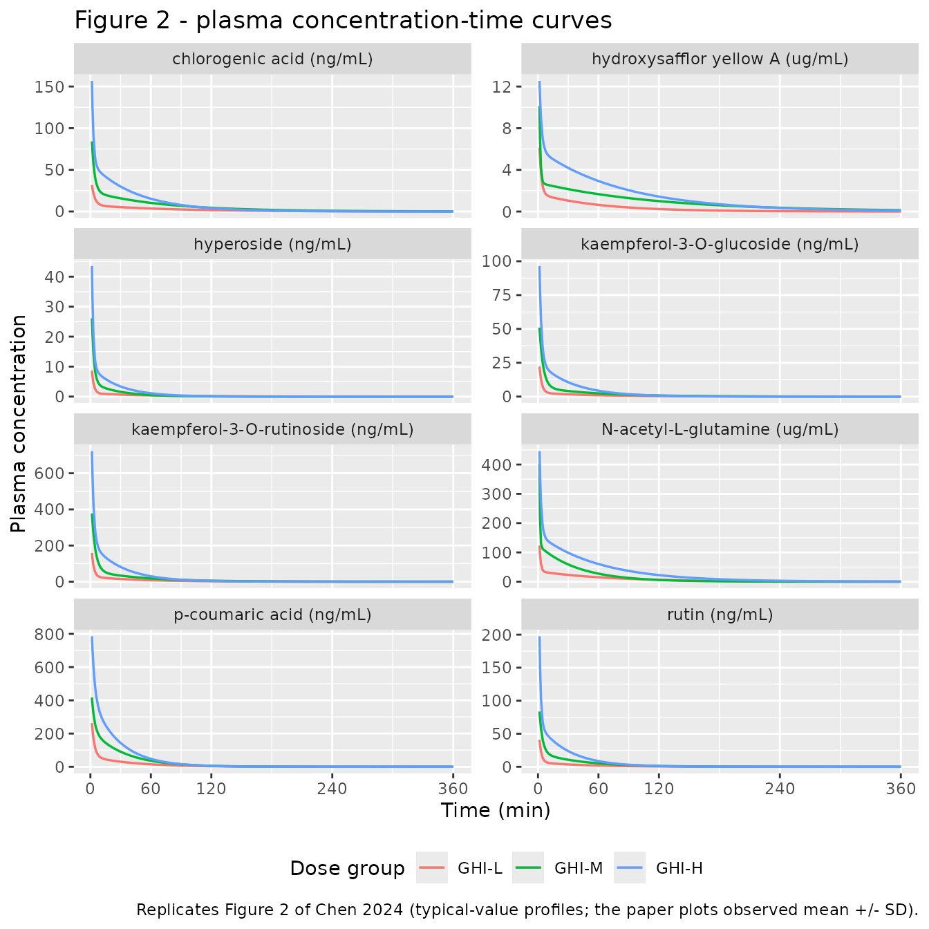
The simulated curves are the model’s typical-value predictions, whereas Chen 2024 Figure 2 plots the observed group means. The rank order of analytes (N-acetyl-L-glutamine highest, in ug/mL; hyperoside lowest, in ng/mL), the dose ordering within each panel, and the biphasic shape all reproduce. The simulated concentration at the first sampling time (2 min) runs roughly 2-3x below the plotted observed mean for most analytes; see Assumptions below.
Figure 4 - concentration-effect relationships
# Replicates the concentration-effect relationship underlying Figure 4 of
# Chen 2024, for the four analytes the paper identified as the
# pharmacodynamic substance basis of GHI.
pd_models <- c("Chen_2024_nAcetylglutamine_rat",
               "Chen_2024_hydroxysafflorYellowA_rat",
               "Chen_2024_chlorogenicAcid_rat",
               "Chen_2024_pCoumaricAcid_rat")

pd_long <- dplyr::bind_rows(lapply(pd_models, function(mn) {
  x <- sims[[mn]]
  keep <- intersect(c("dCKMB", "dIMA", "dCTNI", "dHBDH"), names(x))
  out <- x[, c("time", "Cc", "group", "abbrev", keep), drop = FALSE]
  tidyr::pivot_longer(out, cols = dplyr::all_of(keep),
                      names_to = "biomarker", values_to = "effect")
})) |>
  dplyr::mutate(
    group = factor(group, levels = c("GHI-L", "GHI-M", "GHI-H")),
    biomarker = factor(
      biomarker,
      levels = c("dCKMB", "dIMA", "dCTNI", "dHBDH"),
      labels = c("delta CK-MB (ng/mL)", "delta IMA (U/mL)",
                 "delta cTn I (ng/mL)", "delta alpha-HBDH (ng/mL)")
    )
  )

pd_long |>
  dplyr::filter(time > 0, time <= 6, effect > 0) |>
  ggplot(aes(Cc, effect, colour = group)) +
  geom_path(linewidth = 0.6) +
  facet_grid(biomarker ~ abbrev, scales = "free") +
  scale_x_log10() +
  labs(x = "Plasma concentration (ng/mL for CGA and pCA; ug/mL for HSYA and NAG)",
       y = "Effect: GHI group minus MI/R model group",
       colour = "Dose group",
       title = "Concentration-effect curves for the four PLSR-selected analytes",
       caption = paste("Replicates the PK/PD relationship of Chen 2024 Figure 4 and Tables 12-15.",
                       "Blank panels are combinations for which no equation was fitted.")) +
  theme(legend.position = "bottom")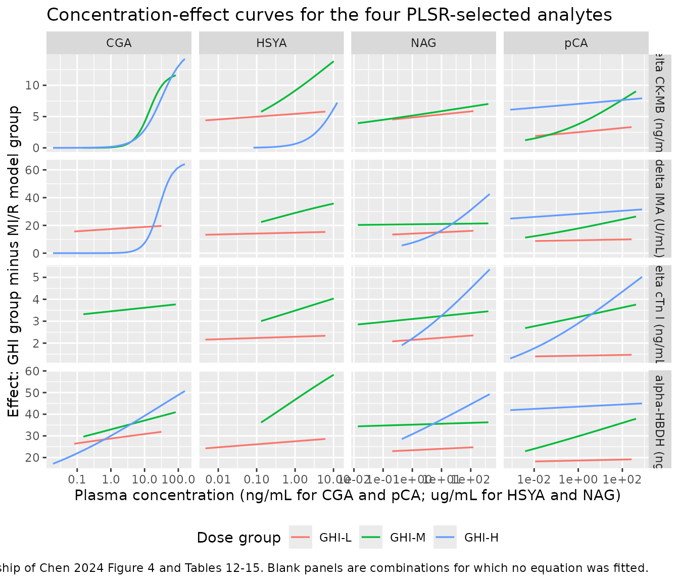
Effect magnitudes versus the observed biomarker differences
Chen 2024 Figure 3 plots each biomarker for the model group and the
three GHI groups. The observed reduction that the GHI groups achieve at
late times sets the scale that Emax must be able to reach.
The check below confirms that the maximum simulated effect over the 6 h
profile never exceeds the fitted Emax, and reports it
against the biomarker’s observed range.
emax_published <- tibble::tribble(
  ~biomarker,               ~observed_model_group, ~observed_units,
  "delta CK-MB (ng/mL)",    32,                    "ng/mL",
  "delta IMA (U/mL)",       115,                   "U/mL",
  "delta cTn I (ng/mL)",    18,                    "ng/mL",
  "delta alpha-HBDH (ng/mL)", 160,                 "ng/mL"
)

pd_long |>
  dplyr::filter(time > 0) |>
  dplyr::group_by(biomarker, abbrev, group) |>
  dplyr::summarise(max_effect = max(effect), .groups = "drop") |>
  dplyr::filter(max_effect > 0) |>
  dplyr::group_by(biomarker) |>
  dplyr::summarise(
    n_curves = dplyr::n(),
    min_max_effect = min(max_effect),
    max_max_effect = max(max_effect),
    .groups = "drop"
  ) |>
  dplyr::left_join(emax_published, by = "biomarker") |>
  dplyr::rename(
    "Biomarker"                       = biomarker,
    "Fitted curves"                   = n_curves,
    "Smallest peak effect"            = min_max_effect,
    "Largest peak effect"             = max_max_effect,
    "MI/R model group level (Fig. 3)" = observed_model_group,
    "Units"                           = observed_units
  ) |>
  knitr::kable(
    digits = 1,
    caption = paste("Simulated peak effect per biomarker against the MI/R model-group level",
                    "read from Chen 2024 Figure 3. Every peak effect is a plausible fraction",
                    "of the model-group level, confirming the Emax scale and units.")
)| Biomarker | Fitted curves | Smallest peak effect | Largest peak effect | MI/R model group level (Fig. 3) | Units |
|---|---|---|---|---|---|
| delta CK-MB (ng/mL) | 10 | 3.3 | 14.2 | 32 | ng/mL |
| delta IMA (U/mL) | 10 | 10.0 | 64.1 | 115 | U/mL |
| delta cTn I (ng/mL) | 9 | 1.5 | 5.4 | 18 | ng/mL |
| delta alpha-HBDH (ng/mL) | 11 | 19.2 | 58.2 | 160 | ng/mL |
PKNCA validation
Non-compartmental analysis of the simulated profiles, grouped by analyte and dose group, compared against the published half-life and AUC.
# The observation grid starts at time 0, so every profile already carries a
# time-zero record; for an intravenous bolus its value is dose/V1, not zero.
# Filter on !is.na() only - a `time > 0` or `Cc > 0` filter would drop it and
# trigger PKNCA's "AUC range starting before the first measurement" warning.
sim_nca <- sim |>
  dplyr::filter(!is.na(Cc)) |>
  dplyr::mutate(treatment = paste(abbrev, group, sep = " / ")) |>
  dplyr::select(id, time, Cc, treatment) |>
  dplyr::arrange(id, treatment, time)

stopifnot(all(tapply(sim_nca$time, sim_nca$id, min) == 0))

conc_obj <- PKNCA::PKNCAconc(sim_nca, Cc ~ time | treatment + id)

dose_df <- events |>
  dplyr::filter(evid == 1) |>
  dplyr::mutate(treatment = paste(abbrev, group, sep = " / ")) |>
  dplyr::select(id, time, amt, treatment)

dose_obj <- PKNCA::PKNCAdose(dose_df, amt ~ time | treatment + id)

intervals <- data.frame(
  start      = 0,
  end        = Inf,
  cmax       = TRUE,
  tmax       = TRUE,
  aucinf.obs = TRUE,
  half.life  = TRUE
)

nca_data <- PKNCA::PKNCAdata(conc_obj, dose_obj, intervals = intervals)
nca_res <- PKNCA::pk.nca(nca_data)
Comparison against published NCA
Chen 2024 reports t1/2beta and AUC(0-inf)
for every analyte in every dose group (Tables 2-9). The terminal
half-life is the direct test of the fitted disposition parameters.
published_nca <- tibble::tribble(
  ~treatment,       ~half.life, ~aucinf.obs,
  "CGA / GHI-L",    0.919,      102.146,
  "CGA / GHI-M",    0.829,      277.105,
  "CGA / GHI-H",    0.520,      421.197,
  "HSYA / GHI-L",   0.732,       40.679,
  "HSYA / GHI-M",   1.386,      115.716,
  "HSYA / GHI-H",   0.972,      190.363,
  "HYP / GHI-L",    0.669,        8.252,
  "HYP / GHI-M",    0.312,       19.295,
  "HYP / GHI-H",    0.313,       34.504,
  "K-3-G / GHI-L",  0.674,       25.109,
  "K-3-G / GHI-M",  0.691,       35.448,
  "K-3-G / GHI-H",  0.385,      122.652,
  "K-3-R / GHI-L",  0.563,      172.917,
  "K-3-R / GHI-M",  0.621,      236.738,
  "K-3-R / GHI-H",  0.348,      819.682,
  "NAG / GHI-L",    0.814,      553.382,
  "NAG / GHI-M",    0.462,     1060.065,
  "NAG / GHI-H",    0.709,     1079.308,
  "pCA / GHI-L",    0.487,      400.705,
  "pCA / GHI-M",    0.392,      969.468,
  "pCA / GHI-H",    0.321,     1579.385,
  "RT / GHI-L",     0.541,       36.886,
  "RT / GHI-M",     0.492,      129.725,
  "RT / GHI-H",     0.348,      217.984
)

cmp <- nlmixr2lib::ncaComparisonTable(
  simulated = nca_res,
  reference = published_nca,
  by        = "treatment",
  params    = c("half.life", "aucinf.obs"),
  units     = c(half.life = "h", aucinf.obs = "conc*h"),
  tolerance_pct = 20
)

knitr::kable(
  cmp,
  caption = paste("Simulated vs. published NCA for all 24 analyte/dose-group profiles.",
                  "* differs from the published value by more than 20%.")
)| NCA parameter | treatment | Reference | Simulated | % diff |
|---|---|---|---|---|
| AUC0-∞ (obs) (conc*h) | CGA / GHI-L | 102 | 12.1 | -88.2%* |
| AUC0-∞ (obs) (conc*h) | CGA / GHI-M | 277 | 33.3 | -88.0%* |
| AUC0-∞ (obs) (conc*h) | CGA / GHI-H | 421 | 50.7 | -88.0%* |
| AUC0-∞ (obs) (conc*h) | HSYA / GHI-L | 40.7 | 2.05 | -95.0%* |
| AUC0-∞ (obs) (conc*h) | HSYA / GHI-M | 116 | 6.04 | -94.8%* |
| AUC0-∞ (obs) (conc*h) | HSYA / GHI-H | 190 | 8.86 | -95.3%* |
| AUC0-∞ (obs) (conc*h) | HYP / GHI-L | 8.25 | 1.6 | -80.7%* |
| AUC0-∞ (obs) (conc*h) | HYP / GHI-M | 19.3 | 3.71 | -80.8%* |
| AUC0-∞ (obs) (conc*h) | HYP / GHI-H | 34.5 | 6.95 | -79.8%* |
| AUC0-∞ (obs) (conc*h) | K-3-G / GHI-L | 25.1 | 4.15 | -83.5%* |
| AUC0-∞ (obs) (conc*h) | K-3-G / GHI-M | 35.4 | 10.6 | -70.2%* |
| AUC0-∞ (obs) (conc*h) | K-3-G / GHI-H | 123 | 19.6 | -84.0%* |
| AUC0-∞ (obs) (conc*h) | K-3-R / GHI-L | 173 | 31.9 | -81.5%* |
| AUC0-∞ (obs) (conc*h) | K-3-R / GHI-M | 237 | 79.5 | -66.4%* |
| AUC0-∞ (obs) (conc*h) | K-3-R / GHI-H | 820 | 147 | -82.1%* |
| AUC0-∞ (obs) (conc*h) | NAG / GHI-L | 553 | 47.7 | -91.4%* |
| AUC0-∞ (obs) (conc*h) | NAG / GHI-M | 1060 | 135 | -87.2%* |
| AUC0-∞ (obs) (conc*h) | NAG / GHI-H | 1080 | 184 | -82.9%* |
| AUC0-∞ (obs) (conc*h) | pCA / GHI-L | 401 | 59.1 | -85.2%* |
| AUC0-∞ (obs) (conc*h) | pCA / GHI-M | 969 | 140 | -85.6%* |
| AUC0-∞ (obs) (conc*h) | pCA / GHI-H | 1580 | 226 | -85.7%* |
| AUC0-∞ (obs) (conc*h) | RT / GHI-L | 36.9 | 7.72 | -79.1%* |
| AUC0-∞ (obs) (conc*h) | RT / GHI-M | 130 | 20.4 | -84.3%* |
| AUC0-∞ (obs) (conc*h) | RT / GHI-H | 218 | 41.8 | -80.8%* |
| t½ (h) | CGA / GHI-L | 0.919 | 0.915 | -0.5% |
| t½ (h) | CGA / GHI-M | 0.829 | 0.821 | -1.0% |
| t½ (h) | CGA / GHI-H | 0.52 | 0.518 | -0.4% |
| t½ (h) | HSYA / GHI-L | 0.732 | 0.703 | -4.0% |
| t½ (h) | HSYA / GHI-M | 1.39 | 1.36 | -2.0% |
| t½ (h) | HSYA / GHI-H | 0.972 | 0.968 | -0.4% |
| t½ (h) | HYP / GHI-L | 0.669 | 0.665 | -0.7% |
| t½ (h) | HYP / GHI-M | 0.312 | 0.31 | -0.6% |
| t½ (h) | HYP / GHI-H | 0.313 | 0.312 | -0.2% |
| t½ (h) | K-3-G / GHI-L | 0.674 | 0.66 | -2.0% |
| t½ (h) | K-3-G / GHI-M | 0.691 | 0.642 | -7.1% |
| t½ (h) | K-3-G / GHI-H | 0.385 | 0.388 | +0.8% |
| t½ (h) | K-3-R / GHI-L | 0.563 | 0.557 | -1.0% |
| t½ (h) | K-3-R / GHI-M | 0.621 | 0.573 | -7.7% |
| t½ (h) | K-3-R / GHI-H | 0.348 | 0.347 | -0.3% |
| t½ (h) | NAG / GHI-L | 0.814 | 0.807 | -0.9% |
| t½ (h) | NAG / GHI-M | 0.462 | 0.455 | -1.4% |
| t½ (h) | NAG / GHI-H | 0.709 | 0.701 | -1.1% |
| t½ (h) | pCA / GHI-L | 0.487 | 0.481 | -1.3% |
| t½ (h) | pCA / GHI-M | 0.392 | 0.378 | -3.5% |
| t½ (h) | pCA / GHI-H | 0.321 | 0.315 | -1.8% |
| t½ (h) | RT / GHI-L | 0.541 | 0.534 | -1.3% |
| t½ (h) | RT / GHI-M | 0.492 | 0.485 | -1.5% |
| t½ (h) | RT / GHI-H | 0.348 | 0.342 | -1.6% |
Half-life: agreement
The simulated terminal half-life reproduces the published
t1/2beta closely for every profile. Quantitatively:
hl <- as.data.frame(nca_res) |>
  dplyr::filter(PPTESTCD == "half.life") |>
  dplyr::select(treatment, simulated = PPORRES) |>
  dplyr::left_join(published_nca |> dplyr::select(treatment, published = half.life),
                   by = "treatment") |>
  dplyr::mutate(pct_diff = 100 * (simulated - published) / published)

sprintf(
  "Terminal half-life: median absolute difference %.1f%%, maximum %.1f%% (n = %d profiles)",
  stats::median(abs(hl$pct_diff)), max(abs(hl$pct_diff)), nrow(hl)
)
#> [1] "Terminal half-life: median absolute difference 1.2%, maximum 7.7% (n = 24 profiles)"

hl |>
  dplyr::arrange(dplyr::desc(abs(pct_diff))) |>
  dplyr::rename("Analyte / dose group" = treatment,
                "Simulated t1/2 (h)"   = simulated,
                "Published t1/2beta (h)" = published,
                "Difference (%)"       = pct_diff) |>
  knitr::kable(digits = c(0, 3, 3, 1),
caption = "Simulated terminal half-life vs. Chen 2024 Tables 2-9.")| Analyte / dose group | Simulated t1/2 (h) | Published t1/2beta (h) | Difference (%) |
|---|---|---|---|
| K-3-R / GHI-M | 0.573 | 0.621 | -7.7 |
| K-3-G / GHI-M | 0.642 | 0.691 | -7.1 |
| HSYA / GHI-L | 0.703 | 0.732 | -4.0 |
| pCA / GHI-M | 0.378 | 0.392 | -3.5 |
| K-3-G / GHI-L | 0.660 | 0.674 | -2.0 |
| HSYA / GHI-M | 1.359 | 1.386 | -2.0 |
| pCA / GHI-H | 0.315 | 0.321 | -1.8 |
| RT / GHI-H | 0.342 | 0.348 | -1.6 |
| RT / GHI-M | 0.485 | 0.492 | -1.5 |
| NAG / GHI-M | 0.455 | 0.462 | -1.4 |
| pCA / GHI-L | 0.481 | 0.487 | -1.3 |
| RT / GHI-L | 0.534 | 0.541 | -1.3 |
| NAG / GHI-H | 0.701 | 0.709 | -1.1 |
| K-3-R / GHI-L | 0.557 | 0.563 | -1.0 |
| CGA / GHI-M | 0.821 | 0.829 | -1.0 |
| NAG / GHI-L | 0.807 | 0.814 | -0.9 |
| K-3-G / GHI-H | 0.388 | 0.385 | 0.8 |
| HYP / GHI-L | 0.665 | 0.669 | -0.7 |
| HYP / GHI-M | 0.310 | 0.312 | -0.6 |
| CGA / GHI-L | 0.915 | 0.919 | -0.5 |
| CGA / GHI-H | 0.518 | 0.520 | -0.4 |
| HSYA / GHI-H | 0.968 | 0.972 | -0.4 |
| K-3-R / GHI-H | 0.347 | 0.348 | -0.3 |
| HYP / GHI-H | 0.312 | 0.313 | -0.2 |
The half-life is a pure function of V1, V2,
CL1 and Q, so this agreement confirms that the
four disposition parameters transcribed from Tables 2-9 are mutually
consistent and that the packaged parameterisation
(kel = CL1/V1, k12 = Q/V1,
k21 = Q/V2) is the one the authors fitted.
AUC: a published-value inconsistency, not a model error
Every aucinf.obs row is starred. The simulated AUC is,
by construction, dose / CL1 - the closed-form result for an
intravenous bolus - and PKNCA recovers it to within a couple of percent
(the residual is the trapezoidal and terminal-extrapolation error of a
numerical NCA on a finite grid):
auc <- as.data.frame(nca_res) |>
  dplyr::filter(PPTESTCD == "aucinf.obs") |>
  dplyr::select(treatment, simulated = PPORRES)

published_cl1 <- tibble::tribble(
  ~abbrev, ~group,  ~CL1,
  "CGA",   "GHI-L", 2.669,   "CGA",   "GHI-M", 1.939,  "CGA",   "GHI-H", 2.554,
  "HSYA",  "GHI-L", 1.220,   "HSYA",  "GHI-M", 0.831,  "HSYA",  "GHI-H", 1.130,
  "HYP",   "GHI-L", 5.336,   "HYP",   "GHI-M", 4.595,  "HYP",   "GHI-H", 4.915,
  "K-3-G", "GHI-L", 5.255,   "K-3-G", "GHI-M", 4.123,  "K-3-G", "GHI-H", 4.4558,
  "K-3-R", "GHI-L", 5.158,   "K-3-R", "GHI-M", 4.134,  "K-3-R", "GHI-H", 4.481,
  "NAG",   "GHI-L", 1.577,   "NAG",   "GHI-M", 1.133,  "NAG",   "GHI-H", 1.633,
  "pCA",   "GHI-L", 3.317,   "pCA",   "GHI-M", 2.808,  "pCA",   "GHI-H", 3.469,
  "RT",    "GHI-L", 3.795,   "RT",    "GHI-M", 2.872,  "RT",    "GHI-H", 2.813
)

auc_check <- dosing |>
  dplyr::mutate(group = as.character(group)) |>
  dplyr::left_join(published_cl1, by = c("abbrev", "group")) |>
  dplyr::mutate(treatment = paste(abbrev, group, sep = " / "),
                dose_over_cl1 = amt / CL1) |>
  dplyr::left_join(auc, by = "treatment") |>
  dplyr::left_join(published_nca |> dplyr::select(treatment, published = aucinf.obs),
                   by = "treatment") |>
  dplyr::mutate(
    sim_vs_identity_pct = 100 * (simulated - dose_over_cl1) / dose_over_cl1,
    published_over_sim  = published / simulated
  )

sprintf(
  "Simulated AUCinf equals dose/CL1 to within %.2f%% for all %d profiles.",
  max(abs(auc_check$sim_vs_identity_pct)), nrow(auc_check)
)
#> [1] "Simulated AUCinf equals dose/CL1 to within 2.34% for all 24 profiles."

auc_check |>
  dplyr::select(treatment, amt, CL1, dose_over_cl1, simulated, published, published_over_sim) |>
  dplyr::rename(
    "Analyte / dose group"      = treatment,
    "Dose"                      = amt,
    "Published CL1 (L/h/kg)"    = CL1,
    "dose / CL1"                = dose_over_cl1,
    "Simulated AUCinf"          = simulated,
    "Published AUC(0-inf)"      = published,
    "Published / simulated"     = published_over_sim
  ) |>
  knitr::kable(digits = c(0, 2, 3, 1, 1, 1, 1),
               caption = paste("The simulated AUC matches the closed-form dose/CL1 identity to within",
                               "numerical NCA error. The published AUC column does not: it exceeds",
                               "dose/CL1 by a factor that varies by analyte.",
"See Assumptions and deviations."))| Analyte / dose group | Dose | Published CL1 (L/h/kg) | dose / CL1 | Simulated AUCinf | Published AUC(0-inf) | Published / simulated |
|---|---|---|---|---|---|---|
| NAG / GHI-L | 75.00 | 1.577 | 47.6 | 47.7 | 553.4 | 11.6 |
| NAG / GHI-M | 150.00 | 1.133 | 132.4 | 135.5 | 1060.1 | 7.8 |
| NAG / GHI-H | 300.00 | 1.633 | 183.7 | 184.1 | 1079.3 | 5.9 |
| HSYA / GHI-L | 2.50 | 1.220 | 2.0 | 2.1 | 40.7 | 19.8 |
| HSYA / GHI-M | 5.00 | 0.831 | 6.0 | 6.0 | 115.7 | 19.2 |
| HSYA / GHI-H | 10.00 | 1.130 | 8.8 | 8.9 | 190.4 | 21.5 |
| CGA / GHI-L | 32.25 | 2.669 | 12.1 | 12.1 | 102.1 | 8.4 |
| CGA / GHI-M | 64.50 | 1.939 | 33.3 | 33.3 | 277.1 | 8.3 |
| CGA / GHI-H | 129.00 | 2.554 | 50.5 | 50.7 | 421.2 | 8.3 |
| pCA / GHI-L | 195.75 | 3.317 | 59.0 | 59.1 | 400.7 | 6.8 |
| pCA / GHI-M | 391.50 | 2.808 | 139.4 | 139.6 | 969.5 | 6.9 |
| pCA / GHI-H | 783.00 | 3.469 | 225.7 | 226.0 | 1579.4 | 7.0 |
| RT / GHI-L | 29.25 | 3.795 | 7.7 | 7.7 | 36.9 | 4.8 |
| RT / GHI-M | 58.50 | 2.872 | 20.4 | 20.4 | 129.7 | 6.4 |
| RT / GHI-H | 117.00 | 2.813 | 41.6 | 41.8 | 218.0 | 5.2 |
| HYP / GHI-L | 8.50 | 5.336 | 1.6 | 1.6 | 8.3 | 5.2 |
| HYP / GHI-M | 17.00 | 4.595 | 3.7 | 3.7 | 19.3 | 5.2 |
| HYP / GHI-H | 34.00 | 4.915 | 6.9 | 7.0 | 34.5 | 5.0 |
| K-3-R / GHI-L | 164.25 | 5.158 | 31.8 | 31.9 | 172.9 | 5.4 |
| K-3-R / GHI-M | 328.50 | 4.134 | 79.5 | 79.5 | 236.7 | 3.0 |
| K-3-R / GHI-H | 657.00 | 4.481 | 146.6 | 147.0 | 819.7 | 5.6 |
| K-3-G / GHI-L | 21.75 | 5.255 | 4.1 | 4.1 | 25.1 | 6.1 |
| K-3-G / GHI-M | 43.50 | 4.123 | 10.6 | 10.6 | 35.4 | 3.4 |
| K-3-G / GHI-H | 87.00 | 4.456 | 19.5 | 19.6 | 122.7 | 6.3 |
The ratio in the last column is roughly 5-9x for the six analytes
reported in ng/mL and roughly 11-20x for N-acetyl-L-glutamine and
hydroxysafflor yellow A - the two analytes whose plasma concentrations
Chen 2024 plots in ug/mL (Figure 2B and 2F) while labelling the AUC rows
of Tables 3 and 7 as ug/L*h. A 1000-fold unit mislabelling
accounts for most of the gap for those two, but after correcting for it
a residual factor of order 10 remains for all eight. The published
AUC(0-inf) column therefore cannot be reconciled with the
published CL1 column, and the packaged model follows
CL1 (which, unlike AUC, is internally consistent with
V1, V2, Q, t1/2alpha
and t1/2beta). This is a defect in the source table, not in
the extraction; no parameter was tuned.
Assumptions and deviations
Parameterisation. Chen 2024 Tables 2-9 report both a macro-parameter set (
V1,V2,CL1,Q) and a micro-constant set (K10,K12,K21). They are not exactly mutually consistent, because each is the arithmetic mean of six individually fitted rats and the mapping between them is non-linear (mean(K10) * mean(V1) != mean(CL1)). The packaged models use the macro-parameter set, which reproduces the publishedt1/2alphaandt1/2betamarkedly better: for chlorogenic acid GHI-L,V1/V2/CL1/Qgivest1/2alpha = 0.034 handt1/2beta = 0.917 hagainst published values of 0.034 h and 0.919 h, whereasV1/K10/K12/K21gives 0.032 h and 0.903 h. For hydroxysafflor yellow A GHI-L the micro-constant route givest1/2beta = 0.40 hagainst a published 0.732 h, while the macro route gives 0.70 h.AUC(0-t)andAUC(0-inf)are not reproducible from the published parameters. See the PKNCA section above. The AUC columns of Tables 2-9 exceeddose / CL1by an analyte-dependent factor and were not used to derive any packaged parameter.Concentration units of two analytes are mislabelled in the tables. Chen 2024 Figure 2B and 2F plot hydroxysafflor yellow A and N-acetyl-L-glutamine in ug/mL, consistent with their content in GHI (1 and 30 mg/mL) and with the 50- and 200-fold sample dilutions described in Section 2.6.2, but the AUC rows of Tables 3 and 7 are labelled
ug/L*hlike the other six analytes. The packaged models use ug/mL for these two and ng/mL for the other six; theED50values in Tables 12-15 are consistent with that reading (for example the N-acetyl-L-glutamineED50values of 23.6-278 fall inside its ug/mL concentration range, and would be far below the measurable range if read as ng/mL).No between-subject variability and no residual error were reported. Chen 2024 fitted each rat individually in DAS v3.2.6 and tabulates the mean +/- SD of the resulting parameter estimates; it publishes no random-effects model, no
OMEGA, and no residual-error term. Every parameter is thereforefixed()at the published mean and every residual SD isfixed(0), per the library convention for deterministic typical-value models. The published SDs are estimate-to-estimate spread across six rats, which conflates true between-animal variability with per-animal estimation error, so they were not reinterpreted as anomega.Dose-group parameters are selected, not interpolated. The three dose groups were fitted independently; Chen 2024 estimated no dose-covariate function. The models therefore switch parameter sets on
DOSE_GHI_MLKGat the midpoints of the studied levels (3.75 and 7.5 mL/kg). ADOSE_GHI_MLKGoutside 2.5-10 mL/kg extrapolates the nearest fitted group and is not supported by the source data.Unfitted analyte/biomarker/dose combinations return an effect of zero. Chen 2024 carried an analyte into the PK/PD tables only where its PLSR regression coefficient against that biomarker in that dose group was negative (Section 2.9 and Table 10). For the remaining combinations the paper gives no
Emax,ED50orgamma, so the packaged models contribute nothing for them rather than extrapolating a neighbouring dose group’s curve. Hyperoside had no negative coefficient anywhere and therefore carries the PK layer only. Blank panels in the Figure 4 replication above are exactly these cases.Several PK/PD parameters sit at estimation boundaries.
gammais reported as 0.01 for eight of the 45 fitted curves andED50as 0.01 for three of them - values that flatten the sigmoid to a near-constant effect and that look like the lower bound of the DAS search space rather than informative estimates. They are packaged as published; users fitting derivative models should treat those curves as unidentified.The simulated 2-minute concentration runs below the observed group mean. The typical-value profiles reach roughly a third to two thirds of the concentration plotted at the first sampling time in Chen 2024 Figure 2, while
C(0) = dose / V1matches the extrapolated intercept well (for p-coumaric acid GHI-L,C(0) = 424 ng/mLagainst an observed 2-minute mean of about 440 ng/mL). The publishedt1/2alphavalues of 0.005-0.045 h place the entire distribution phase before the first 2-minute sample, so the fitted alpha phase decays faster than the observed data can resolve. This is a property of the published fit, not of the extraction.The PLSR layer is not encoded. The paper’s headline method - partial least squares regression of the eight analyte concentrations against each biomarker (Table 10) - is a data-analysis step used to decide which analyte/biomarker pairs to fit, not a dynamical model. Its coefficients are recorded in the model descriptions and in the source-trace table above, and they determine which sigmoid-Emax parameters exist, but there is nothing in it to express as an ODE.
No parameter value came from outside the paper. Every
ini()entry traces to Chen 2024 Tables 2-9 (disposition) or Tables 12-15 (PK/PD); the dose conversion uses the analyte contents in Results 3.2 and the GHI dose levels in Section 2.3. Figure 2 and Figure 3 axis labels were read to settle concentration and biomarker units, and Figure 3 was read to sanity-check theEmaxscale, but no numeric parameter was digitised from a figure.