Piperacillin-tazobactam in critically ill adults (Reeder 2025)
Source:vignettes/articles/Reeder_2025_piperacillin_tazobactam.Rmd
Reeder_2025_piperacillin_tazobactam.RmdModel and source
- Citation: Reeder JA, Creech CB, Nation RL, Gu K, Nalbant D, Wu N, Jimenez-Truque N, Fissell W, Rolsma S, Fishbane N, Kirkpatrick C, Patel P, Watanabe A, Landersdorfer C, Winokur P, An G (2025). Utilizing an Opportunistic Clinical Study and Population-Based Pharmacokinetic Models to Identify Rational Empiric Dosing Regimens for Piperacillin-Tazobactam in Critically Ill Patients. The Journal of Clinical Pharmacology 65(4):452-465. doi:10.1002/jcph.6161.
- Piperacillin model: One-compartment population PK model with linear elimination for the piperacillin component of intravenously infused piperacillin-tazobactam in critically ill adults in the ICU (Reeder 2025; 111 patients, 239 plasma concentrations from opportunistic sampling). Outside continuous renal replacement therapy (CRRT), clearance is the sum of a renal arm proportional to Cockcroft-Gault creatinine clearance on lean body weight and a non-renal arm scaling with lean body weight to the 0.75 power; in patients on CRRT a single estimated CRRT clearance replaces both arms. Uncorrelated interindividual variability on total clearance and volume and a combined proportional plus additive residual error. The companion tazobactam model is Reeder_2025_tazobactam.
- Tazobactam model: One-compartment population PK model with linear elimination for the tazobactam component of intravenously infused piperacillin-tazobactam in critically ill adults in the ICU (Reeder 2025; 108 patients, 229 plasma concentrations from opportunistic sampling). Clearance is the sum of a renal arm proportional to Cockcroft-Gault creatinine clearance on lean body weight and a constant non-renal arm; in patients on continuous renal replacement therapy (CRRT) an estimated CRRT clearance replaces the renal arm while the non-renal arm is retained. Uncorrelated interindividual variability on total clearance and volume and a combined proportional plus additive residual error. The companion piperacillin model is Reeder_2025_piperacillin.
- Article: https://doi.org/10.1002/jcph.6161 (open access, PMC11938006)
Reeder et al. fitted two separate one-compartment population PK
models, one for piperacillin and one for tazobactam, to
opportunistically sampled plasma concentrations from critically ill
adults receiving piperacillin-tazobactam as 4-hour extended infusions.
The models are packaged as Reeder_2025_piperacillin and
Reeder_2025_tazobactam. Both use Cockcroft-Gault creatinine
clearance computed on lean body weight (CRCL, mL/min) and a
continuous renal replacement therapy indicator
(RRT_CRRT_STATUS); piperacillin additionally uses lean body
weight (LBM, kg) on its non-renal clearance.
Population
112 critically ill adults were enrolled in the ICUs of the University of Iowa and Vanderbilt University Medical Center (Table 1 of the paper). Median age was 64 years (range 21-88), 45% were female, and 90% were white. Median total body weight was 92 kg (41-160) and median lean body weight 57 kg (30-89). Median Cockcroft-Gault creatinine clearance was 82 mL/min (10-289) on total body weight and 51 mL/min (8-173) on lean body weight. 26% had acute kidney injury, 33% sepsis, 27% septic shock and 39% were mechanically ventilated; 10 patients (8.9%) were on continuous renal replacement therapy (8 CVVHDF, 2 CVVH). All but one patient received 3375 mg piperacillin-tazobactam (3000 mg / 375 mg) as 4-hour infusions, mostly every 8 hours (Table S1). After outlier removal the piperacillin analysis used 239 concentrations from 111 patients and the tazobactam analysis 229 concentrations from 108 patients.
The same information is available programmatically:
str(rxode2::rxode(readModelDb("Reeder_2025_piperacillin"))$population[
  c("n_subjects", "age_median", "weight_median", "sex_female_pct")
])
#> ℹ parameter labels from comments will be replaced by 'label()'
#> List of 4
#>  $ n_subjects    : int 111
#>  $ age_median    : chr "64 years"
#>  $ weight_median : chr "92 kg total body weight; 57 kg lean body weight"
#>  $ sex_female_pct: num 45
Source trace
Every ini() value carries an in-file comment pointing to
its source. The table collects them.
| Model | Equation / parameter | Value | Source location |
|---|---|---|---|
| piperacillin | lcl_renal |
log(1.97 L/h) | Table 2, CLR (RSE 29%) |
| piperacillin | lcl_nonren |
log(2.58 L/h) | Table 2, CLNR (RSE 27%) |
| piperacillin | lcl_crrt |
log(3.32 L/h) | Table 2, CLCRRT = CLT,CRRT (RSE 12%); footnote a |
| piperacillin | lvc |
log(23.5 L) | Table 2, V (RSE 10%) |
| piperacillin | e_crcl_cl_renal |
1.00, held constant | Table 2, CLR * (CLCR,LBW/51 mL/min)^theta
|
| piperacillin | e_lbm_cl_nonren |
0.75, held constant | Table 2, CLNR * (LBW/57 kg)^theta
|
| piperacillin | etalcl |
0.1996 (47% CV) | Table 2, IIV CL; footnote c (total CL) |
| piperacillin | etalvc |
0.1034 (33% CV) | Table 2, IIV V |
| piperacillin |
propSd, addSd
|
0.39, 0.326 mg/L | Table 2, CVCP and SDCP |
| piperacillin | CL equation | ((CLR + CLNR) (1 - CRRT) + CLCRRT CRRT) exp(eta) |
Table 2 footnotes a and c |
| tazobactam | lcl_renal |
log(2.38 L/h) | Table 2, CLR (RSE 23%) |
| tazobactam | lcl_nonren |
log(1.63 L/h) | Table 2, CLNR (RSE 38%) |
| tazobactam | lcl_crrt |
log(0.957 L/h) | Table 2, CLCRRT (RSE 70%) |
| tazobactam | lvc |
log(25.3 L) | Table 2, V (RSE 14%) |
| tazobactam | e_crcl_cl_renal |
1.00, held constant | Table 2, CLR * (CLCR,LBW/51 mL/min)^theta
|
| tazobactam | etalcl |
0.1484 (40% CV) | Table 2, IIV CL; footnote c (total CL) |
| tazobactam | etalvc |
0.0975 (32% CV) | Table 2, IIV V |
| tazobactam |
propSd, addSd
|
0.40, 0.255 mg/L | Table 2, CVCP and SDCP |
| tazobactam | CL equation | (CLR (1 - CRRT) + CLNR + CLCRRT CRRT) exp(eta) |
Table 2 footnotes b and c |
| both | d/dt(central) <- -kel * central |
n/a | Results, “one-compartment model with zero-order input and first-order elimination” |
| both | Cc ~ add(addSd) + prop(propSd) |
n/a | Results, “combined proportional and additive error model” |
Typical-value check against Table 2
Table 2 also prints the derived total clearances at the reference covariates (CLcr,LBW 51 mL/min, LBW 57 kg). Solving the packaged models with the random effects removed must reproduce them to the printed precision.
mod_pip <- readModelDb("Reeder_2025_piperacillin")
mod_taz <- readModelDb("Reeder_2025_tazobactam")

ref_ev <- data.frame(
  id = 1:2, time = 0, evid = 1, amt = 1000, rate = 250, cmt = "central",
  CRCL = 51, LBM = 57, RRT_CRRT_STATUS = c(0, 1)
) |>
  dplyr::bind_rows(data.frame(
    id = 1:2, time = 1, evid = 0, amt = 0, rate = 0, cmt = "central",
    CRCL = 51, LBM = 57, RRT_CRRT_STATUS = c(0, 1)
  )) |>
  dplyr::arrange(id, time)

typ <- function(mod, drug) {
  rxode2::rxSolve(rxode2::zeroRe(mod), events = ref_ev) |>
    as.data.frame() |>
    dplyr::distinct(id, cl) |>
    dplyr::mutate(drug = drug, CRRT = c("no", "yes")[id])
}
typ_tab <- dplyr::bind_rows(
  typ(mod_pip, "piperacillin"),
  typ(mod_taz, "tazobactam")
) |>
  dplyr::mutate(published = c(4.55, 3.32, 4.01, 2.59))
#> ℹ parameter labels from comments will be replaced by 'label()'
#> ℹ omega/sigma items treated as zero: 'etalcl', 'etalvc'
#> Warning: multi-subject simulation without without 'omega'
#> ℹ parameter labels from comments will be replaced by 'label()'
#> ℹ omega/sigma items treated as zero: 'etalcl', 'etalvc'
#> Warning: multi-subject simulation without without 'omega'

typ_tab |>
  dplyr::select(drug, CRRT, cl, published) |>
  dplyr::rename(
    "Drug" = drug, "On CRRT" = CRRT,
    "Model CL (L/h)" = cl, "Table 2 CLT (L/h)" = published
  ) |>
knitr::kable(digits = 3)| Drug | On CRRT | Model CL (L/h) | Table 2 CLT (L/h) |
|---|---|---|---|
| piperacillin | no | 4.550 | 4.55 |
| piperacillin | yes | 3.320 | 3.32 |
| tazobactam | no | 4.010 | 4.01 |
| tazobactam | yes | 2.587 | 2.59 |
Virtual cohort
The individual patient data are not public. The virtual cohort below approximates Table 1: lean body weight log-normal around the 57 kg median and clipped to the observed 30-89 kg range; Cockcroft-Gault creatinine clearance on lean body weight proportional to lean body weight (as the Cockcroft-Gault formula makes it) times a log-normal factor, centred on 51 mL/min and clipped to 8-173 mL/min; total body weight as lean body weight times a log-normal ratio centred on 92/57, clipped to 41-160 kg. 9% of subjects (18 of 200) are on CRRT, drawn from the lowest-clearance third of the cohort. Total body weight is used only to form the total-body-weight creatinine clearance used to stratify the target-attainment tables; it does not enter either model.
Between-subject random effects are drawn in base R from each model’s
omega matrix and passed through params = to the models with
the random effects zeroed, so the cohort is identical on every machine
and every dosing regimen is simulated on the same 200 virtual
patients.
set.seed(20250325)
n_sub <- 200L

clip <- function(x, lo, hi) pmin(pmax(x, lo), hi)
cohort <- tibble::tibble(k = seq_len(n_sub)) |>
  dplyr::mutate(
    LBM = clip(exp(rnorm(n_sub, log(57), 0.22)), 30, 89),
    CRCL = clip(51 * (LBM / 57) * exp(rnorm(n_sub, 0, 0.61)), 8, 173),
    WT = clip(LBM * exp(rnorm(n_sub, log(92 / 57), 0.15)), 41, 160),
    CRCL_TBW = CRCL * WT / LBM
  )
low_third <- which(cohort$CRCL <= quantile(cohort$CRCL, 1 / 3))
cohort$RRT_CRRT_STATUS <- 0
cohort$RRT_CRRT_STATUS[sample(low_third, 18)] <- 1

draw_eta <- function(mod, n) {
  omega <- rxode2::rxode2(mod)$omega
  eta <- matrix(rnorm(n * nrow(omega)), n) %*% chol(omega)
  colnames(eta) <- rownames(omega)
  as.data.frame(eta)
}
eta_pip <- draw_eta(mod_pip, n_sub)
#> ℹ parameter labels from comments will be replaced by 'label()'
eta_taz <- draw_eta(mod_taz, n_sub)
#> ℹ parameter labels from comments will be replaced by 'label()'

cohort |>
  dplyr::summarise(
    `LBW median (range), kg` = sprintf("%.0f (%.0f-%.0f)", median(LBM), min(LBM), max(LBM)),
    `TBW median (range), kg` = sprintf("%.0f (%.0f-%.0f)", median(WT), min(WT), max(WT)),
    `CLcr,LBW median (range), mL/min` = sprintf("%.0f (%.0f-%.0f)", median(CRCL), min(CRCL), max(CRCL)),
    `CLcr,TBW median (range), mL/min` = sprintf("%.0f (%.0f-%.0f)", median(CRCL_TBW), min(CRCL_TBW), max(CRCL_TBW)),
    `CRRT, n (%)` = sprintf("%d (%.1f%%)", sum(RRT_CRRT_STATUS), 100 * mean(RRT_CRRT_STATUS))
  ) |>
  tidyr::pivot_longer(dplyr::everything(), names_to = "Covariate", values_to = "Virtual cohort") |>
  dplyr::mutate(`Table 1` = c("57 (30-89)", "92 (41-160)", "51 (8-173)", "82 (10-289)", "10 (8.9%)")) |>
knitr::kable()| Covariate | Virtual cohort | Table 1 |
|---|---|---|
| LBW median (range), kg | 56 (31-89) | 57 (30-89) |
| TBW median (range), kg | 93 (42-160) | 92 (41-160) |
| CLcr,LBW median (range), mL/min | 50 (9-173) | 51 (8-173) |
| CLcr,TBW median (range), mL/min | 85 (15-357) | 82 (10-289) |
| CRRT, n (%) | 18 (9.0%) | 10 (8.9%) |
Piperacillin probability of target attainment (Figure 3, Table 3)
The paper simulated 20 piperacillin regimens: 2, 3 or 4 g every 6, 8 or 12 h as 0.5-hour intermittent or 4-hour extended infusions, and 6, 9, 12 or 16 g per day as a continuous infusion. Free concentrations were the total concentrations times 0.70 (30% protein binding). Here each regimen is simulated for 48 hours and the target 100% fT > MIC is evaluated over the second day (24-48 h): a subject attains the target at a given MIC when its lowest free concentration in that window exceeds the MIC.
regimens <- dplyr::bind_rows(
  tidyr::expand_grid(
    dose_g = c(2, 3, 4), tau = c(6, 8, 12), dur = c(0.5, 4)
  ) |>
    dplyr::filter(!(dose_g == 2 & tau == 12)),
  tibble::tibble(dose_g = c(6, 9, 12, 16), tau = 24, dur = 24)
) |>
  dplyr::mutate(
    infusion = dplyr::case_when(
      dur == 0.5 ~ "Intermittent (0.5 h)",
      dur == 4 ~ "Extended (4 h)",
      TRUE ~ "Continuous (24 h)"
    ),
    regimen = ifelse(
      dur == 24,
      sprintf("%gg qd 24-h infusion", dose_g),
      sprintf("%gg q%gh %s infusion", dose_g, tau, ifelse(dur == 0.5, "30-min", "4-h"))
    ),
    r = dplyr::row_number()
  )
stopifnot(nrow(regimens) == 20)

make_events <- function(reg, cohort, obs_times) {
  subj <- cohort |>
    dplyr::mutate(id = (reg$r - 1L) * nrow(cohort) + k)
  doses <- tidyr::expand_grid(subj, time = seq(0, 48 - reg$tau, by = reg$tau)) |>
    dplyr::mutate(evid = 1, amt = reg$dose_g * 1000, rate = amt / reg$dur)
  obs <- tidyr::expand_grid(subj, time = obs_times) |>
    dplyr::mutate(evid = 0, amt = 0, rate = 0)
  dplyr::bind_rows(doses, obs) |>
    dplyr::mutate(cmt = "central", regimen = reg$regimen, infusion = reg$infusion)
}
ev_pta <- lapply(split(regimens, regimens$r), make_events,
  cohort = cohort, obs_times = seq(24, 48, by = 0.25)
) |>
  dplyr::bind_rows() |>
  dplyr::arrange(id, time, dplyr::desc(evid))
stopifnot(!anyDuplicated(ev_pta[ev_pta$evid == 0, c("id", "time")]))

# params rows must follow the ascending id order of the event table.
params_pta <- dplyr::bind_cols(
  id = sort(unique(ev_pta$id)),
  eta_pip[rep(seq_len(n_sub), nrow(regimens)), , drop = FALSE]
)
sim_pta <- rxode2::rxSolve(
  rxode2::zeroRe(mod_pip),
  events = ev_pta, params = params_pta,
  keep = c("regimen", "infusion", "CRCL_TBW")
) |>
  as.data.frame()
#> ℹ parameter labels from comments will be replaced by 'label()'
#> Warning: multi-subject simulation without without 'omega'

mic_grid <- 2^(-3:7) # 0.125 to 128 mg/L
fu_pip <- 0.70

min_free <- sim_pta |>
  dplyr::group_by(id, regimen, infusion, CRCL, CRCL_TBW) |>
  dplyr::summarise(cmin_free = min(fu_pip * Cc), .groups = "drop")

pta_by <- function(df, ...) {
  df |>
    dplyr::group_by(regimen, infusion, ...) |>
    dplyr::reframe(MIC = mic_grid, PTA = sapply(mic_grid, function(m) mean(cmin_free > m)))
}
breakpoint <- function(pta) {
  pta |>
    dplyr::summarise(
      bp = if (any(PTA >= 0.9)) max(MIC[PTA >= 0.9]) else 0.0625,
      .groups = "drop"
    )
}
pta_all <- pta_by(min_free)
# Replicates Figure 3 of Reeder 2025: PTA versus MIC for 100% fT > MIC.
pta_all |>
  dplyr::mutate(infusion = factor(infusion, levels = c(
    "Intermittent (0.5 h)", "Extended (4 h)", "Continuous (24 h)"
  ))) |>
  ggplot(aes(MIC, 100 * PTA, colour = regimen)) +
  geom_line() +
  geom_point(size = 1) +
  geom_hline(yintercept = 90, linetype = "dashed") +
  scale_x_continuous(trans = "log2", breaks = mic_grid, labels = as.character(mic_grid)) +
  facet_wrap(~infusion, ncol = 1) +
  labs(
    x = "MIC (mg/L)", y = "PTA (%)", colour = NULL,
    title = "Piperacillin PTA, target 100% fT > MIC",
    caption = "Replicates Figure 3 of Reeder 2025 (200 virtual patients per regimen)."
  ) +
  theme_bw() +
  theme(legend.position = "right")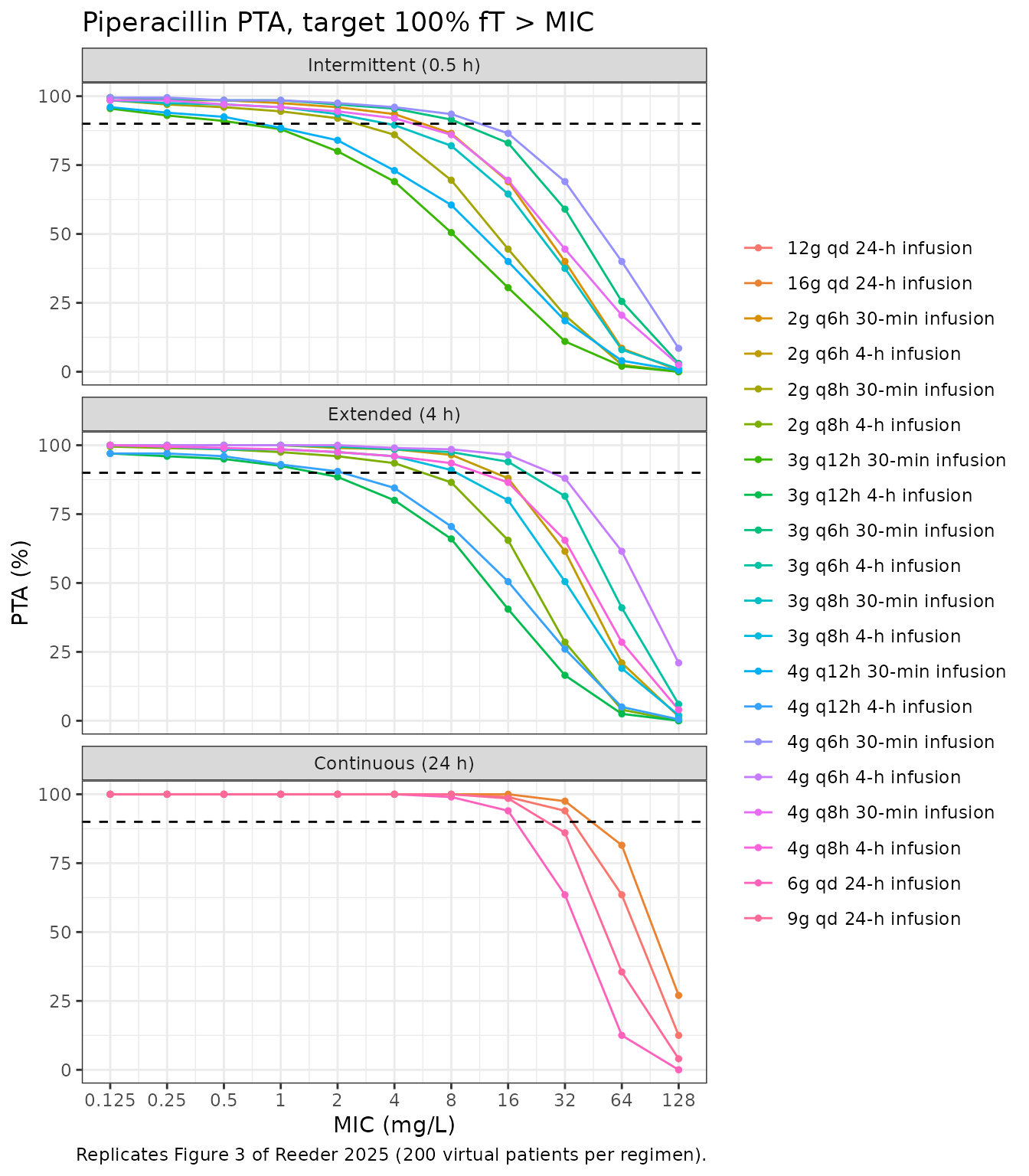
The breakpoint is the highest MIC at which at least 90% of patients attain the target. Table 3 of the paper gives it for the whole population and by creatinine-clearance band.
published_all <- tibble::tribble(
  ~regimen, ~bp_paper,
  "2g q6h 30-min infusion", 4, "2g q8h 30-min infusion", 2,
  "3g q6h 30-min infusion", 8, "3g q8h 30-min infusion", 4,
  "3g q12h 30-min infusion", 1, "4g q6h 30-min infusion", 8,
  "4g q8h 30-min infusion", 4, "4g q12h 30-min infusion", 1,
  "2g q6h 4-h infusion", 8, "2g q8h 4-h infusion", 4,
  "3g q6h 4-h infusion", 16, "3g q8h 4-h infusion", 8,
  "3g q12h 4-h infusion", 2, "4g q6h 4-h infusion", 16,
  "4g q8h 4-h infusion", 8, "4g q12h 4-h infusion", 2,
  "6g qd 24-h infusion", 16, "9g qd 24-h infusion", 16,
  "12g qd 24-h infusion", 32, "16g qd 24-h infusion", 32
)
cmp_all <- breakpoint(pta_all |> dplyr::group_by(regimen)) |>
  dplyr::inner_join(published_all, by = "regimen") |>
  dplyr::mutate(dilutions = log2(bp / bp_paper)) |>
  dplyr::arrange(match(regimen, published_all$regimen))
stopifnot(nrow(cmp_all) == 20)

cmp_all |>
  dplyr::rename(
    "Regimen" = regimen, "Simulated breakpoint (mg/L)" = bp,
    "Table 3 breakpoint (mg/L)" = bp_paper, "Difference (doubling dilutions)" = dilutions
  ) |>
knitr::kable(caption = "Piperacillin breakpoints, all patients, target 100% fT > MIC.")| Regimen | Simulated breakpoint (mg/L) | Table 3 breakpoint (mg/L) | Difference (doubling dilutions) |
|---|---|---|---|
| 2g q6h 30-min infusion | 4.0 | 4 | 0 |
| 2g q8h 30-min infusion | 2.0 | 2 | 0 |
| 3g q6h 30-min infusion | 8.0 | 8 | 0 |
| 3g q8h 30-min infusion | 2.0 | 4 | -1 |
| 3g q12h 30-min infusion | 0.5 | 1 | -1 |
| 4g q6h 30-min infusion | 8.0 | 8 | 0 |
| 4g q8h 30-min infusion | 4.0 | 4 | 0 |
| 4g q12h 30-min infusion | 0.5 | 1 | -1 |
| 2g q6h 4-h infusion | 8.0 | 8 | 0 |
| 2g q8h 4-h infusion | 4.0 | 4 | 0 |
| 3g q6h 4-h infusion | 16.0 | 16 | 0 |
| 3g q8h 4-h infusion | 8.0 | 8 | 0 |
| 3g q12h 4-h infusion | 1.0 | 2 | -1 |
| 4g q6h 4-h infusion | 16.0 | 16 | 0 |
| 4g q8h 4-h infusion | 8.0 | 8 | 0 |
| 4g q12h 4-h infusion | 2.0 | 2 | 0 |
| 6g qd 24-h infusion | 16.0 | 16 | 0 |
| 9g qd 24-h infusion | 16.0 | 16 | 0 |
| 12g qd 24-h infusion | 32.0 | 32 | 0 |
| 16g qd 24-h infusion | 32.0 | 32 | 0 |
published_strata <- tibble::tribble(
  ~regimen, ~lt60, ~mid, ~ge130,
  "2g q6h 30-min infusion", 8, 4, 2, "2g q8h 30-min infusion", 8, 2, 0.5,
  "3g q6h 30-min infusion", 16, 8, 2, "3g q8h 30-min infusion", 8, 2, 0.5,
  "3g q12h 30-min infusion", 4, 0.5, 0.0625, "4g q6h 30-min infusion", 16, 8, 4,
  "4g q8h 30-min infusion", 16, 4, 1, "4g q12h 30-min infusion", 4, 0.5, 0.125,
  "2g q6h 4-h infusion", 16, 8, 4, "2g q8h 4-h infusion", 8, 4, 2,
  "3g q6h 4-h infusion", 32, 16, 8, "3g q8h 4-h infusion", 16, 8, 2,
  "3g q12h 4-h infusion", 4, 1, 0.25, "4g q6h 4-h infusion", 32, 16, 8,
  "4g q8h 4-h infusion", 16, 8, 4, "4g q12h 4-h infusion", 8, 2, 0.25,
  "6g qd 24-h infusion", 16, 8, 8, "9g qd 24-h infusion", 32, 16, 8,
  "12g qd 24-h infusion", 32, 16, 16, "16g qd 24-h infusion", 64, 32, 16
) |>
  tidyr::pivot_longer(-regimen, names_to = "band", values_to = "bp_paper")

band_of <- function(x) {
  dplyr::case_when(x < 60 ~ "lt60", x < 130 ~ "mid", TRUE ~ "ge130")
}
strata_cmp <- dplyr::bind_rows(
  min_free |> dplyr::mutate(band = band_of(CRCL_TBW), basis = "CLcr,TBW"),
  min_free |> dplyr::mutate(band = band_of(CRCL), basis = "CLcr,LBW")
) |>
  pta_by(band, basis) |>
  dplyr::group_by(regimen, band, basis) |>
  breakpoint() |>
  dplyr::inner_join(published_strata, by = c("regimen", "band")) |>
  dplyr::mutate(dilutions = log2(bp / bp_paper))

strata_cmp |>
  dplyr::group_by(basis) |>
  dplyr::summarise(
    `Median difference (dilutions)` = median(dilutions),
    `Within 1 dilution (%)` = 100 * mean(abs(dilutions) <= 1),
    .groups = "drop"
  ) |>
  dplyr::rename("Band variable" = basis) |>
knitr::kable(caption = "Agreement with the Table 3 creatinine-clearance bands (<60, 60-129, >=130 mL/min) under either Cockcroft-Gault body-weight basis.")| Band variable | Median difference (dilutions) | Within 1 dilution (%) |
|---|---|---|
| CLcr,LBW | 0 | 75 |
| CLcr,TBW | 0 | 100 |
strata_cmp |>
  dplyr::filter(basis == "CLcr,TBW") |>
  dplyr::mutate(band = factor(band, c("lt60", "mid", "ge130"), c("<60", "60-129", ">=130"))) |>
  dplyr::select(regimen, band, bp, bp_paper) |>
  tidyr::pivot_wider(names_from = band, values_from = c(bp, bp_paper)) |>
  dplyr::arrange(match(regimen, published_all$regimen)) |>
  dplyr::select(
    regimen, `bp_<60`, `bp_paper_<60`, `bp_60-129`, `bp_paper_60-129`,
    `bp_>=130`, `bp_paper_>=130`
  ) |>
  dplyr::rename(
    "Regimen" = regimen,
    "Sim <60" = `bp_<60`, "Paper <60" = `bp_paper_<60`,
    "Sim 60-129" = `bp_60-129`, "Paper 60-129" = `bp_paper_60-129`,
    "Sim >=130" = `bp_>=130`, "Paper >=130" = `bp_paper_>=130`
  ) |>
knitr::kable(caption = "Piperacillin breakpoints (mg/L) by CLcr band, banded on total-body-weight Cockcroft-Gault clearance. Paper values below 0.125 mg/L are shown as 0.0625.")| Regimen | Sim <60 | Paper <60 | Sim 60-129 | Paper 60-129 | Sim >=130 | Paper >=130 |
|---|---|---|---|---|---|---|
| 2g q6h 30-min infusion | 8 | 8 | 8 | 4.0 | 1.0000 | 2.0000 |
| 2g q8h 30-min infusion | 4 | 8 | 4 | 2.0 | 0.2500 | 0.5000 |
| 3g q6h 30-min infusion | 16 | 16 | 8 | 8.0 | 2.0000 | 2.0000 |
| 3g q8h 30-min infusion | 8 | 8 | 4 | 2.0 | 0.5000 | 0.5000 |
| 3g q12h 30-min infusion | 2 | 4 | 1 | 0.5 | 0.0625 | 0.0625 |
| 4g q6h 30-min infusion | 16 | 16 | 16 | 8.0 | 2.0000 | 4.0000 |
| 4g q8h 30-min infusion | 8 | 16 | 8 | 4.0 | 0.5000 | 1.0000 |
| 4g q12h 30-min infusion | 2 | 4 | 1 | 0.5 | 0.0625 | 0.1250 |
| 2g q6h 4-h infusion | 16 | 16 | 16 | 8.0 | 4.0000 | 4.0000 |
| 2g q8h 4-h infusion | 8 | 8 | 8 | 4.0 | 1.0000 | 2.0000 |
| 3g q6h 4-h infusion | 32 | 32 | 16 | 16.0 | 8.0000 | 8.0000 |
| 3g q8h 4-h infusion | 16 | 16 | 8 | 8.0 | 2.0000 | 2.0000 |
| 3g q12h 4-h infusion | 4 | 4 | 2 | 1.0 | 0.1250 | 0.2500 |
| 4g q6h 4-h infusion | 32 | 32 | 32 | 16.0 | 8.0000 | 8.0000 |
| 4g q8h 4-h infusion | 16 | 16 | 16 | 8.0 | 2.0000 | 4.0000 |
| 4g q12h 4-h infusion | 4 | 8 | 2 | 2.0 | 0.2500 | 0.2500 |
| 6g qd 24-h infusion | 16 | 16 | 16 | 8.0 | 8.0000 | 8.0000 |
| 9g qd 24-h infusion | 32 | 32 | 16 | 16.0 | 16.0000 | 8.0000 |
| 12g qd 24-h infusion | 32 | 32 | 32 | 16.0 | 16.0000 | 16.0000 |
| 16g qd 24-h infusion | 64 | 64 | 32 | 32.0 | 32.0000 | 16.0000 |
Banding on total-body-weight Cockcroft-Gault clearance puts every stratified breakpoint within one doubling dilution of Table 3, against three quarters when banding on the lean-body-weight form, which suggests Table 3 bands on the total-body-weight clearance.
# The virtual cohort only approximates the study's covariate distribution, and
# breakpoints move in two-fold steps, so the gate is on agreement in the
# centre: a mis-transcribed clearance or volume shifts every breakpoint by one
# or more dilutions in the same direction.
stopifnot(
  abs(median(cmp_all$dilutions)) <= 0.5,
  mean(abs(cmp_all$dilutions) <= 1) >= 0.8
)
Tazobactam free-concentration profiles (Figure 5)
The paper simulated tazobactam 0.5 g every 8 hours as 0.5-hour and as 4-hour infusions and 1.5 g per day as a continuous infusion, with a free fraction of 0.70, and compared the free concentrations with a 4 mg/L minimum critical concentration.
taz_regimens <- tibble::tibble(
  r = 1:3, dose_g = c(0.5, 0.5, 1.5), tau = c(8, 8, 24), dur = c(0.5, 4, 24),
  regimen = c("0.5 g q8h (0.5-h infusion)", "0.5 g q8h (4-h infusion)", "1.5 g qd (24-h infusion)"),
  infusion = regimen
)
ev_taz <- lapply(split(taz_regimens, taz_regimens$r), make_events,
  cohort = cohort, obs_times = seq(0, 48, by = 0.25)
) |>
  dplyr::bind_rows() |>
  dplyr::arrange(id, time, dplyr::desc(evid))
params_taz <- dplyr::bind_cols(
  id = sort(unique(ev_taz$id)),
  eta_taz[rep(seq_len(n_sub), nrow(taz_regimens)), , drop = FALSE]
)
sim_taz <- rxode2::rxSolve(
  rxode2::zeroRe(mod_taz),
  events = ev_taz, params = params_taz, keep = "regimen"
) |>
  as.data.frame() |>
  dplyr::mutate(Cfree = 0.70 * Cc)
#> ℹ parameter labels from comments will be replaced by 'label()'
#> Warning: multi-subject simulation without without 'omega'

taz_q <- sim_taz |>
  dplyr::group_by(regimen, time) |>
  dplyr::summarise(
    Q05 = quantile(Cfree, 0.05), Q50 = median(Cfree), Q95 = quantile(Cfree, 0.95),
    .groups = "drop"
  )
# Replicates Figure 5 of Reeder 2025.
ggplot(taz_q, aes(time)) +
  geom_line(aes(y = Q50)) +
  geom_line(aes(y = Q05), linetype = "dashed", colour = "blue") +
  geom_line(aes(y = Q95), linetype = "dashed", colour = "blue") +
  geom_hline(yintercept = 4, colour = "red", linetype = "dotdash") +
  facet_wrap(~regimen, ncol = 1) +
  scale_x_continuous(breaks = seq(0, 48, 8)) +
  labs(
    x = "Time (h)", y = "Tazobactam free concentration (mg/L)",
    title = "Simulated tazobactam free concentrations, median and 5th/95th percentiles",
    caption = "Replicates Figure 5 of Reeder 2025; red line = 4 mg/L threshold."
  ) +
  theme_bw()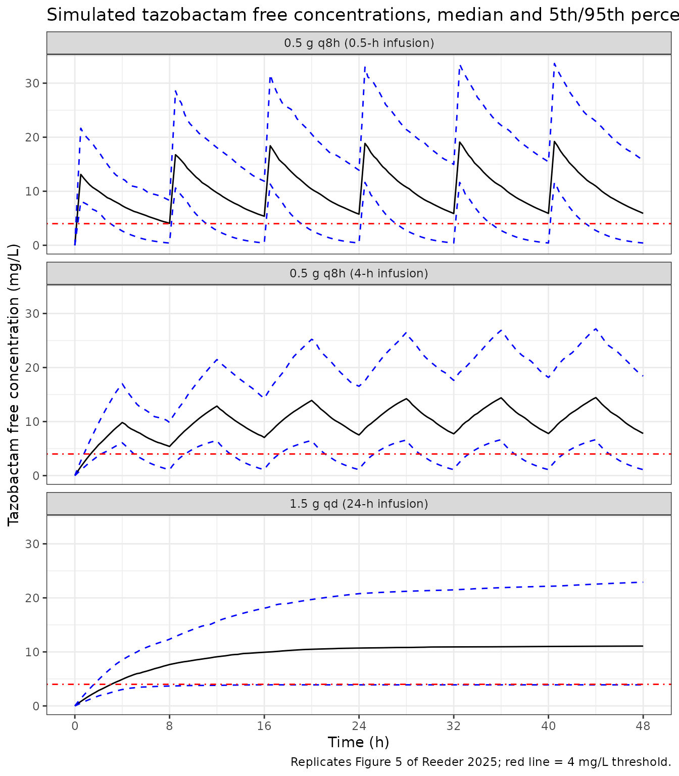
The figure’s continuous-infusion panel plateaus at about 10.9 mg/L
(median), 4.3 mg/L (5th percentile) and 25.7 mg/L (95th percentile) by
48 hours, read off Figure 5c by the maintainers. The typical patient’s
steady-state free concentration is
0.70 x 62.5 mg/h / 4.01 L/h = 10.9 mg/L, so the median of
the published figure sits exactly on the model’s typical value.
taz_48 <- taz_q |>
  dplyr::filter(time == 48, regimen == "1.5 g qd (24-h infusion)")
taz_cmp <- tibble::tibble(
  Statistic = c("5th percentile", "Median", "95th percentile"),
  Simulated = c(taz_48$Q05, taz_48$Q50, taz_48$Q95),
  `Figure 5c (digitised)` = c(4.3, 10.9, 25.7)
) |>
  dplyr::mutate(`Difference (%)` = 100 * (Simulated / `Figure 5c (digitised)` - 1))
knitr::kable(taz_cmp, digits = 1, caption = "Tazobactam free concentration at 48 h, 1.5 g/day continuous infusion.")| Statistic | Simulated | Figure 5c (digitised) | Difference (%) |
|---|---|---|---|
| 5th percentile | 3.9 | 4.3 | -9.3 |
| Median | 11.1 | 10.9 | 1.6 |
| 95th percentile | 22.9 | 25.7 | -10.9 |
# The median tracks clearance and dose directly; the tails also depend on how
# well the virtual covariate distribution matches the real one, so they get a
# wider envelope.
stopifnot(
  abs(taz_cmp$`Difference (%)`[2]) < 15,
  all(abs(taz_cmp$`Difference (%)`) < 40)
)

# Paper: >95% of patients above 4 mg/L on the continuous infusion and more
# than half above it throughout the dosing interval on either 0.5 g q8h form.
above_mcc <- sim_taz |>
  dplyr::filter(time >= 24) |>
  dplyr::group_by(regimen, id) |>
  dplyr::summarise(above = all(Cfree > 4), .groups = "drop") |>
  dplyr::group_by(regimen) |>
  dplyr::summarise(`Patients above 4 mg/L throughout 24-48 h (%)` = 100 * mean(above))
above_mcc |>
  dplyr::rename("Regimen" = regimen) |>
knitr::kable(digits = 1)| Regimen | Patients above 4 mg/L throughout 24-48 h (%) |
|---|---|
| 0.5 g q8h (0.5-h infusion) | 69.0 |
| 0.5 g q8h (4-h infusion) | 78.5 |
| 1.5 g qd (24-h infusion) | 94.0 |
The paper states that more than half of patients stay above 4 mg/L throughout the interval on both 0.5 g q8h regimens and more than 95% on the continuous infusion. The simulated continuous-infusion attainment sits just below 95%, consistent with the simulated 5th percentile at 48 h (3.9 mg/L) lying just below the published one (4.3 mg/L); the virtual cohort’s creatinine-clearance tail is slightly wider than the study’s.
Steady-state NCA for the studied regimen (PKNCA)
The study regimen was 3375 mg piperacillin-tazobactam (3000 mg / 375 mg) as a 4-hour infusion every 8 hours. Simulating 15 doses and running PKNCA on the last dosing interval gives the steady-state exposure of each component. The paper reports no NCA, so the check is internal: at steady state the AUC over one dosing interval equals dose / CL for every subject.
nca_events <- function(drug_dose, cohort, offset) {
  subj <- cohort |> dplyr::mutate(id = offset + k)
  doses <- tidyr::expand_grid(subj, time = seq(0, 112, by = 8)) |>
    dplyr::mutate(evid = 1, amt = drug_dose, rate = drug_dose / 4)
  obs <- tidyr::expand_grid(subj, time = seq(112, 120, by = 0.25)) |>
    dplyr::mutate(evid = 0, amt = 0, rate = 0)
  dplyr::bind_rows(doses, obs) |>
    dplyr::mutate(cmt = "central") |>
    dplyr::arrange(id, time, dplyr::desc(evid))
}
ss_solve <- function(mod, eta, drug_dose, drug) {
  ev <- nca_events(drug_dose, cohort, 0L) |> dplyr::mutate(treatment = drug)
  rxode2::rxSolve(
    rxode2::zeroRe(mod),
    events = ev, keep = "treatment",
    params = dplyr::bind_cols(id = seq_len(n_sub), eta)
  ) |>
    as.data.frame() |>
    dplyr::mutate(dose = drug_dose)
}
sim_ss <- dplyr::bind_rows(
  ss_solve(mod_pip, eta_pip, 3000, "piperacillin 3000 mg q8h 4-h"),
  ss_solve(mod_taz, eta_taz, 375, "tazobactam 375 mg q8h 4-h")
)
#> ℹ parameter labels from comments will be replaced by 'label()'
#> Warning: multi-subject simulation without without 'omega'
#> ℹ parameter labels from comments will be replaced by 'label()'
#> Warning: multi-subject simulation without without 'omega'

conc_df <- sim_ss |>
  dplyr::filter(!is.na(Cc)) |>
  dplyr::select(id, time, Cc, treatment)
dose_df <- dplyr::bind_rows(
  nca_events(3000, cohort, 0L) |> dplyr::mutate(treatment = "piperacillin 3000 mg q8h 4-h"),
  nca_events(375, cohort, 0L) |> dplyr::mutate(treatment = "tazobactam 375 mg q8h 4-h")
) |>
  dplyr::filter(evid == 1) |>
  dplyr::select(id, time, amt, treatment)

conc_obj <- PKNCA::PKNCAconc(conc_df, Cc ~ time | treatment + id, concu = "mg/L", timeu = "h")
dose_obj <- PKNCA::PKNCAdose(dose_df, amt ~ time | treatment + id, doseu = "mg")
intervals <- data.frame(
  start = 112, end = 120,
  cmax = TRUE, tmax = TRUE, cmin = TRUE, auclast = TRUE, cav = TRUE
)
nca_res <- PKNCA::pk.nca(PKNCA::PKNCAdata(conc_obj, dose_obj, intervals = intervals))
summary(nca_res)
#>  Interval Start Interval End                    treatment   N AUClast (h*mg/L)
#>             112          120 piperacillin 3000 mg q8h 4-h 200       640 [58.7]
#>             112          120    tazobactam 375 mg q8h 4-h 200      92.1 [60.0]
#>  Cmax (mg/L) Cmin (mg/L)          Tmax (h)  Cav (mg/L)
#>   113 [46.0]  41.2 [144] 4.00 [4.00, 4.00] 80.0 [58.7]
#>  15.3 [46.9]  7.06 [118] 4.00 [4.00, 4.00] 11.5 [60.0]
#>
#> Caption: AUClast, Cmax, Cmin, Cav: geometric mean and geometric coefficient of variation; Tmax: median and range; N: number of subjects
auc_chk <- as.data.frame(nca_res$result) |>
  dplyr::filter(PPTESTCD == "auclast") |>
  dplyr::select(treatment, id, auclast = PPORRES) |>
  dplyr::inner_join(
    sim_ss |> dplyr::distinct(treatment, id, cl, dose),
    by = c("treatment", "id")
  ) |>
  dplyr::mutate(pct_diff = 100 * (auclast / (dose / cl) - 1))

auc_chk |>
  dplyr::group_by(treatment) |>
  dplyr::summarise(
    `Median AUCtau (mg*h/L)` = median(auclast),
    `Median dose/CL (mg*h/L)` = median(dose / cl),
    `Median difference (%)` = median(pct_diff),
    `90th pct abs difference (%)` = quantile(abs(pct_diff), 0.9)
  ) |>
  dplyr::rename("Component" = treatment) |>
knitr::kable(digits = 2)| Component | Median AUCtau (mg*h/L) | Median dose/CL (mg*h/L) | Median difference (%) | 90th pct abs difference (%) |
|---|---|---|---|---|
| piperacillin 3000 mg q8h 4-h | 637.11 | 637.17 | -0.01 | 0.05 |
| tazobactam 375 mg q8h 4-h | 95.38 | 95.38 | -0.01 | 0.05 |
# Both sides use the same per-subject parameters, so the residual is the
# approach to steady state after 15 doses plus trapezoidal error on a 0.25-h
# grid (measured: 90th percentile 0.05%). A mis-entered dose, rate or
# clearance moves AUCtau by tens of percent. The slowest-clearance subjects
# are the ones still accumulating, so the gate is on the centre and a robust
# quantile, not the extreme.
stopifnot(
  all(abs(tapply(auc_chk$pct_diff, auc_chk$treatment, median)) < 1),
  all(tapply(abs(auc_chk$pct_diff), auc_chk$treatment, quantile, 0.9) < 3)
)
Assumptions and deviations
- No correlation between the CL and V random effects. The base models estimated a CL-V correlation (Tables S2 and S3), but Table 2 of the final models reports only the two variances and no covariance or correlation, so the packaged models carry independent etas. If the final models retained the correlation, simulated variability in concentrations is somewhat overstated here.
-
Covariate exponents held constant. The 1.00
exponent of creatinine clearance on renal clearance (both drugs) and the
0.75 exponent of lean body weight on piperacillin non-renal clearance
are printed in Table 2 with no RSE and no bootstrap interval, as round
theory values, so they are encoded with
fixed(). - Piperacillin CRRT clearance. Table 2 prints CLCRRT = 3.32 L/h without an RSE and CLT,CRRT = 3.32 L/h (RSE 12%); footnote a states they are the same quantity, so one parameter carries the estimate.
-
Lean body weight formula unknown. The paper does
not name the formula, so the covariate is mapped to the canonical
LBMcolumn. Users should check that their formula reproduces the 57 kg cohort median for a cohort with median total body weight 92 kg. - Virtual cohort. Covariate distributions were approximated from the Table 1 medians and ranges (see above), with CRRT patients drawn from the lowest-clearance third; the paper resampled its own 111 (piperacillin) or 108 (tazobactam) patients 100 times. Simulated breakpoints and percentiles therefore agree with the paper in the centre rather than row by row.
- Target-attainment window. The paper does not state over which interval 100% fT > MIC was assessed; the second day of a 48-hour simulation (24-48 h) is used, matching the 48-hour horizon stated for the tazobactam simulations. Residual error is not added to the simulated concentrations.
- Creatinine-clearance bands. Table 3 does not say whether its bands use creatinine clearance on total or lean body weight. Both are tabulated above; the per-regimen table uses the total-body-weight basis, the conventional basis for an augmented-renal-clearance cut-off of 130 mL/min.
- Figure 5c percentiles were read off the published figure by the maintainers (to about 0.3 mg/L).
- No erratum or correction notice for the paper was found on Europe PMC as of 2026-11-03.