Linezolid (Soraluce 2020)
Source:vignettes/articles/Soraluce_2020_linezolid.Rmd
Soraluce_2020_linezolid.RmdModel and source
- Citation: Soraluce A, Barrasa H, Asin-Prieto E, Sanchez-Izquierdo JA, Maynar J, Isla A, Rodriguez-Gascon A. Novel Population Pharmacokinetic Model for Linezolid in Critically Ill Patients and Evaluation of the Adequacy of the Current Dosing Recommendation. Pharmaceutics. 2020;12(1):54. doi:10.3390/pharmaceutics12010054
- Description: Two-compartment IV population PK model for linezolid in 40 critically ill adults, 23 of them on continuous renal replacement therapy (Soraluce 2020). Total clearance is the sum of an estimated non-renal clearance (2.62 L/h), a renal clearance proportional to urine-measured creatinine clearance (4.35 L/h at 44 mL/min), and the individually measured extracorporeal clearance (sieving coefficient times effluent flow) supplied as the data column QEFF; a single exponential random effect scales the whole sum. Central volume 16.2 L, peripheral volume 29.0 L, intercompartmental clearance 71.7 L/h, with IIV on clearance and central volume and a combined additive + proportional residual error.
- Article: Pharmaceutics. 2020;12(1):54 (open access)
Population
Forty critically ill adults treated with linezolid for a suspected Gram-positive infection in the intensive care units of three Spanish university hospitals (Araba, Doce de Octubre and Joan XXIII). Twenty-three received continuous renal replacement therapy (CRRT; 18 continuous venovenous hemodiafiltration, 5 continuous venovenous hemodialysis) and 17 did not. Infection sources were pulmonary (14), abdominal (10), neurological (9), biliary (2) and other (5). Of the 40 patients, 29 were men. Median age was 72 years (range 22-85) without CRRT and 68 (37-79) with CRRT, and median weight 71 kg (60-95) and 74 kg (55-110) respectively (Table 1).
Renal function was measured, not estimated: creatinine clearance came
from a 10-hour urine collection,
Clcr = (Cru * Vu) / (Crp * 600 min). Median Clcr was 71.2
mL/min (11.0-179.5) without CRRT and 6.0 mL/min (0.0-45.6) with CRRT.
For CRRT patients the extracorporeal clearance
CLEC = Sc * Qef was computed per patient from the measured
sieving coefficient and the effluent flow: median 2.51 L/h
(0.79-3.09).
All patients received 600 mg every 12 h as a 30-min intravenous infusion (one patient 60 min) and were sampled at steady state after a mean of 8 doses: 311 plasma concentrations in total. An external validation cohort of 11 further patients, none on CRRT (median Clcr 111 mL/min, range 45-240; Table 2), received a 600 mg loading dose followed by 50 mg/h by continuous infusion.
The same information is available programmatically via
rxode2::rxode(readModelDb("Soraluce_2020_linezolid"))$population.
Source trace
Every ini() value carries an in-file comment pointing to
its source in
inst/modeldb/specificDrugs/Soraluce_2020_linezolid.R; the
table collects them.
| Equation / parameter | Value | Source location |
|---|---|---|
CL = (CLNR + CLR * (Clcr/44) + Sc * Qef) * exp(eta1) |
n/a | Table 3 footnote b (final model) |
V1 = 16.2 * exp(eta2) |
n/a | Table 3 footnote d |
| Two-compartment, linear elimination | n/a | Results 3.1.1 |
CLEC = Sc * Qef, per-patient data column
(QEFF), CRRT only |
n/a | Section 2.1; Section 2.3.2; Table 3 footnote c |
Clcr from 10-h urine collection |
n/a | Section 2.1 |
lcl_nonren (CLNR) |
2.62 L/h (RSE 18%) | Table 3, final model |
lcl_renal (theta in CLR) |
4.35 L/h at Clcr = 44 mL/min (RSE 19%) | Table 3, final model |
lvc (V1) |
16.2 L (RSE 14%) | Table 3, final model |
lq (Q) |
71.7 L/h (RSE 14%) | Table 3, final model |
lvp (V2) |
29.0 L (RSE 7%) | Table 3, final model |
etalcl |
61.5% -> omega^2 = log(0.615^2 + 1) = 0.3205 | Table 3, final model |
etalvc |
65.9% -> omega^2 = log(0.659^2 + 1) = 0.3606 | Table 3, final model |
| No CL-V1 covariance | n/a | Results 3.1.1 |
addSd |
0.266 mg/L (RSE 24%) | Table 3, final model |
propSd |
0.159 (RSE 19%) | Table 3, final model |
Virtual cohort
The observed data are not public. Two arms of 200 subjects each reproduce the two strata of Table 1 at the standard 600 mg every 12 h, 30-min infusion regimen. Covariates are drawn from log-normal distributions whose medians are the Table 1 medians, truncated to the Table 1 ranges (the paper gives only median and range):
- no CRRT:
CRCLmedian 71.2 mL/min, truncated to 11.0-179.5;QEFF = 0; - CRRT:
CRCLmedian 6.0 mL/min, truncated to 0-45.6;QEFFmedian 2.51 L/h, truncated to 0.79-3.09.
# rxSetSeed() fixes the draw within an rxode2 build but not across builds or
# solver-thread counts; every assertion below is on a closed form or on
# quantities computed from the same drawn parameters, never on a cohort
# extreme.
rxode2::rxSetSeed(20200109)
set.seed(20200109)

N_PER_ARM <- 200L
DOSE <- 600 # mg
TAU <- 12 # h
TINF <- 0.5 # h

rtlnorm <- function(n, median, gsd, lo, hi) {
  pmin(pmax(exp(rnorm(n, log(median), log(gsd))), lo), hi)
}

cohort <- dplyr::bind_rows(
  tibble::tibble(
    id = seq_len(N_PER_ARM),
    arm = "No CRRT",
    CRCL = rtlnorm(N_PER_ARM, 71.2, 1.8, 11.0, 179.5),
    QEFF = 0
  ),
  tibble::tibble(
    id = N_PER_ARM + seq_len(N_PER_ARM),
    arm = "CRRT",
    CRCL = rtlnorm(N_PER_ARM, 6.0, 2.5, 0, 45.6),
    QEFF = rtlnorm(N_PER_ARM, 2.51, 1.4, 0.79, 3.09)
  )
)

cohort |>
  dplyr::group_by(arm) |>
  dplyr::summarise(
    CRCL_median = median(CRCL),
    CRCL_min = min(CRCL),
    CRCL_max = max(CRCL),
    QEFF_median = median(QEFF),
    .groups = "drop"
  )
#> # A tibble: 2 × 5
#>   arm     CRCL_median CRCL_min CRCL_max QEFF_median
#>   <chr>         <dbl>    <dbl>    <dbl>       <dbl>
#> 1 CRRT           5.88    0.495     45.6        2.51
#> 2 No CRRT       71.6    13.9      180.         0

# One steady-state dosing interval per subject, observed on the central state.
# The grid is dense over the first 2 h: subjects in the upper tail of the
# clearance distribution (CL up to ~100 L/h) have a steep post-infusion
# decline, and a coarse grid there leaves a few percent of trapezoidal error
# in the AUC check below.
obs_times <- sort(unique(round(c(seq(0, 2, by = 0.02), seq(2, TAU, by = 0.25)), 6)))
events <- rxode2::et(amt = DOSE, dur = TINF, ii = TAU, ss = 1, cmt = "central") |>
  rxode2::et(obs_times, cmt = "central") |>
  rxode2::et(id = cohort$id) |>
  as.data.frame() |>
  dplyr::left_join(cohort, by = "id")
Simulation
mod <- readModelDb("Soraluce_2020_linezolid")

sim <- rxode2::rxSolve(
  mod,
  events = events,
  keep = c("arm", "CRCL", "QEFF"),
  rtol = 1e-10, atol = 1e-12, ssRtol = 1e-10, ssAtol = 1e-12
) |>
  as.data.frame()
#> ℹ parameter labels from comments will be replaced by 'label()'
Steady-state profiles (compare Figure 2)
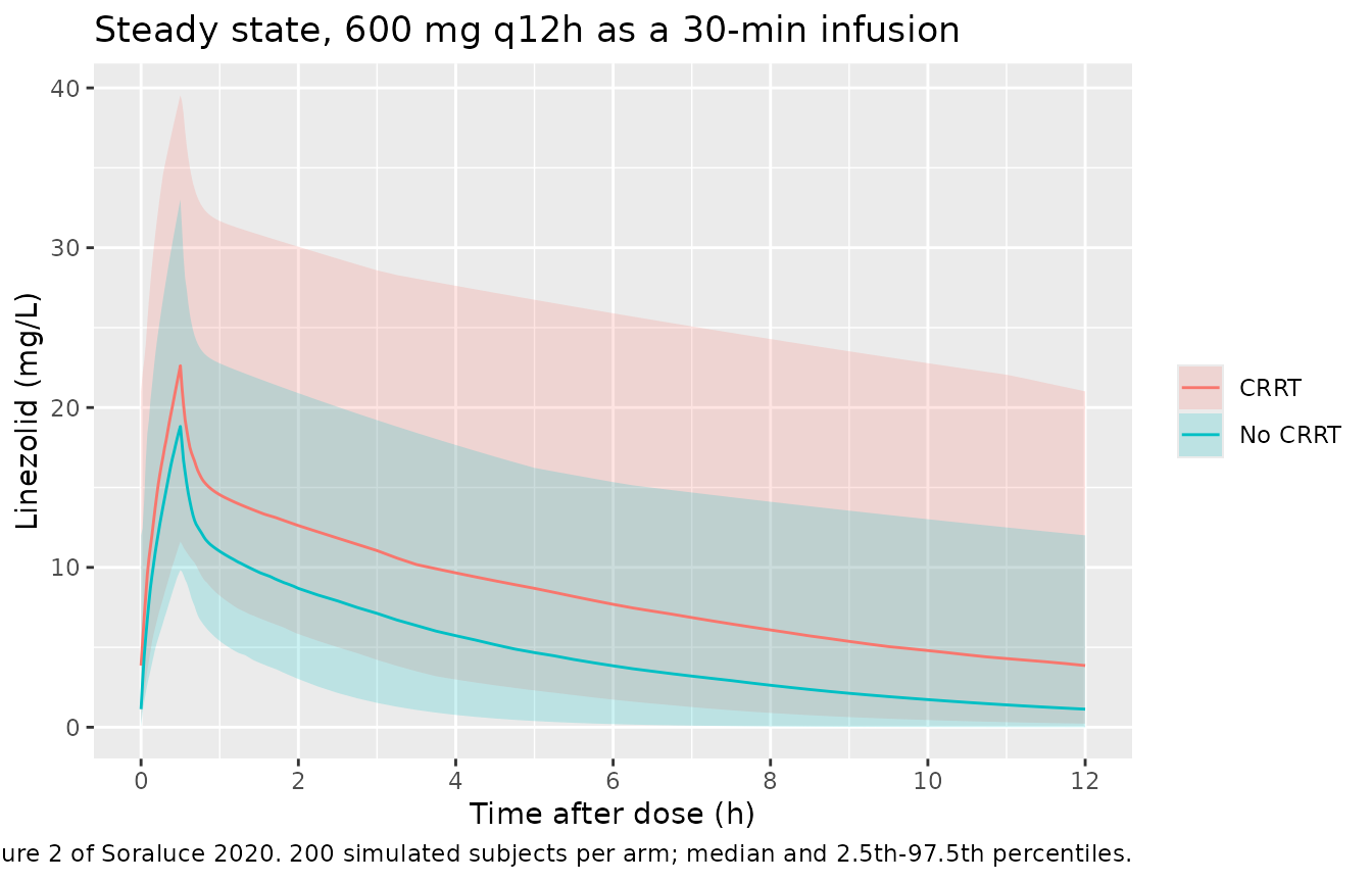
Figure 2 of the paper is a VPC of the observed steady-state interval, 0-12 h after dose, with the observed median peaking near 20 mg/L at the end of the infusion and falling to about 3-5 mg/L at 12 h. The plot below shows the simulated median and 2.5th-97.5th percentile band of the individual predictions for each arm.
vpc <- sim |>
  dplyr::filter(!is.na(Cc)) |>
  dplyr::group_by(arm, time) |>
  dplyr::summarise(
    p025 = quantile(Cc, 0.025),
    p50 = median(Cc),
    p975 = quantile(Cc, 0.975),
    .groups = "drop"
  )

ggplot(vpc, aes(time, p50, colour = arm, fill = arm)) +
  geom_ribbon(aes(ymin = p025, ymax = p975), alpha = 0.2, colour = NA) +
  geom_line() +
  scale_x_continuous(breaks = seq(0, 12, 2)) +
  labs(
    x = "Time after dose (h)", y = "Linezolid (mg/L)", colour = NULL, fill = NULL,
    title = "Steady state, 600 mg q12h as a 30-min infusion",
    caption = paste(
      "Compare Figure 2 of Soraluce 2020.", N_PER_ARM,
      "simulated subjects per arm; median and 2.5th-97.5th percentiles."
    )
  )
PKNCA validation
NCA over the steady-state interval, grouped by arm. At steady state
the area under the curve over one dosing interval equals
Dose / CL exactly, and the simulation reports each
subject’s drawn cl, so the NCA AUC can be checked against
the closed form subject by subject. Both sides use the same drawn
parameters, so the only difference is trapezoidal error on the
observation grid and a tight bound is appropriate.
conc_df <- sim |>
  dplyr::filter(!is.na(Cc)) |>
  dplyr::select(id, time, Cc, arm)

dose_df <- cohort |>
  dplyr::transmute(id, time = 0, amt = DOSE, arm)

conc_obj <- PKNCA::PKNCAconc(conc_df, Cc ~ time | arm + id)
dose_obj <- PKNCA::PKNCAdose(dose_df, amt ~ time | arm + id)

intervals <- data.frame(
  start = 0, end = TAU,
  auclast = TRUE, cmax = TRUE, tmax = TRUE, cmin = TRUE
)

nca <- PKNCA::pk.nca(PKNCA::PKNCAdata(conc_obj, dose_obj, intervals = intervals))
nca_res <- as.data.frame(nca$result)

nca_res |>
  dplyr::group_by(arm, PPTESTCD) |>
  dplyr::summarise(median = signif(median(PPORRES), 3), .groups = "drop") |>
  tidyr::pivot_wider(names_from = PPTESTCD, values_from = median) |>
  dplyr::rename(
    "Arm" = arm,
    "AUC0-12 (mg*h/L)" = auclast,
    "Cmax (mg/L)" = cmax,
    "Cmin (mg/L)" = cmin,
    "Tmax (h)" = tmax
  ) |>
knitr::kable(caption = "Median steady-state NCA parameters by arm (simulated).")| Arm | AUC0-12 (mg*h/L) | Cmax (mg/L) | Cmin (mg/L) | Tmax (h) |
|---|---|---|---|---|
| CRRT | 99.9 | 22.6 | 3.86 | 0.5 |
| No CRRT | 58.9 | 18.8 | 1.13 | 0.5 |
auc_chk <- nca_res |>
  dplyr::filter(PPTESTCD == "auclast") |>
  dplyr::left_join(
    sim |> dplyr::distinct(id, cl),
    by = "id"
  ) |>
  dplyr::mutate(pct_diff = 100 * (PPORRES - DOSE / cl) / (DOSE / cl))

summary(auc_chk$pct_diff)
#>       Min.    1st Qu.     Median       Mean    3rd Qu.       Max.
#> -0.0166031 -0.0011837 -0.0005040 -0.0011011 -0.0001663  0.0001138

# Same drawn parameters on both sides: pure numerical error, so all() is right.
# Dropping the renal or the CRRT arm from the solved clearance would move the
# AUC by tens of percent in one arm or the other.
stopifnot(
  nrow(auc_chk) == 2L * N_PER_ARM,
  all(abs(auc_chk$pct_diff) < 1)
)
The paper reports no NCA parameters for the model-building cohort, so there is no published NCA table to compare against; the comparison against published results is the Figure 3 check below.
Replicate published figures
Figure 3 - continuous infusion, simulated steady-state concentration
The external validation (Section 2.3.4) simulated 5000 subjects at
each of six creatinine clearances (40, 80, 120, 160, 200 and 240 mL/min,
no CRRT) receiving 50 mg/h by continuous infusion, and the inset of
Figure 3 prints the pooled simulated steady-state concentration as
median 3.30 mg/L (2.5th-97.5th percentile 0.85-14.73). At steady state
Css = 50 / CL, independent of the volumes, and with the
single log-normal random effect on the total clearance the pooled
distribution is an equal-weight mixture of six log-normals, whose
quantiles can be computed exactly by root-finding. This makes the
comparison deterministic and therefore able to hold on every
machine.
omega_cl <- 0.320546 # log(0.615^2 + 1)
CRCL_GRID <- c(40, 80, 120, 160, 200, 240)
tv_cl <- 2.62 + 4.35 * CRCL_GRID / 44 # Table 3 footnote b, QEFF = 0

# P(Css <= x) for the pooled six-stratum mixture, Css = 50 / (tv_cl * exp(eta))
p_css <- function(x) {
  mean(stats::pnorm(log(50 / (tv_cl * x)), 0, sqrt(omega_cl), lower.tail = FALSE))
}
q_css <- function(p) {
  stats::uniroot(function(x) p_css(x) - p, c(1e-3, 1e3), tol = 1e-10)$root
}

fig3 <- tibble::tibble(
  statistic = c("median", "2.5th percentile", "97.5th percentile"),
  p = c(0.5, 0.025, 0.975),
  published = c(3.30, 0.85, 14.73)
) |>
  dplyr::rowwise() |>
  dplyr::mutate(model = q_css(p)) |>
  dplyr::ungroup() |>
  dplyr::mutate(pct_diff = 100 * (model - published) / published)

fig3 |>
  dplyr::mutate(model = round(model, 2), pct_diff = round(pct_diff, 1)) |>
  dplyr::select(statistic, model, published, pct_diff) |>
  dplyr::rename(
    "Statistic" = statistic,
    "This model (mg/L)" = model,
    "Figure 3 inset (mg/L)" = published,
    "Difference (%)" = pct_diff
  ) |>
knitr::kable(caption = "Pooled simulated Css at 50 mg/h. Replicates the Figure 3 inset of Soraluce 2020.")| Statistic | This model (mg/L) | Figure 3 inset (mg/L) | Difference (%) |
|---|---|---|---|
| median | 3.27 | 3.30 | -0.8 |
| 2.5th percentile | 0.85 | 0.85 | 0.0 |
| 97.5th percentile | 14.77 | 14.73 | 0.3 |
# Deterministic: a mis-read renal reference (44 mL/min), a dropped renal arm
# or the omega = CV^2 reading moves at least one quantile by far more than 3%.
stopifnot(all(abs(fig3$pct_diff) < 3))
The same calculation on the alternative reading of the IIV column, with the printed 61.5% taken as the standard deviation of eta (omega^2 = 0.615^2), gives a 97.5th percentile of about 15.9 mg/L, 8% above the published 14.73, and a 2.5th percentile of about 0.78 mg/L, 8% below the published 0.85; only the median is unchanged. The log-normal CV reading omega^2 = log(CV^2 + 1) used in the model file reproduces all three printed values, and it also shows that the paper’s percentiles exclude residual error: adding the Table 3 residual error widens the lower tail to about 0.72-0.77 mg/L.
q_alt <- local({
  omega_cl <- 0.615^2
  p_alt <- function(x) {
    mean(stats::pnorm(log(50 / (tv_cl * x)), 0, sqrt(omega_cl), lower.tail = FALSE))
  }
  stats::uniroot(function(x) p_alt(x) - 0.975, c(1e-3, 1e3), tol = 1e-10)$root
})
round(q_alt, 2)
#> [1] 15.88
stopifnot(abs(100 * (q_alt - 14.73) / 14.73) > 5)
A stochastic simulation of the same design checks that the ODE model itself reaches the analytic steady state: 600 mg over 30 min, then 50 mg/h, with concentrations over the 12-108 h window that Figure 3 plots. It uses 100 subjects per clearance stratum.
N_STRATUM <- 100L
ci_cohort <- tidyr::expand_grid(CRCL = CRCL_GRID, k = seq_len(N_STRATUM)) |>
  dplyr::mutate(id = dplyr::row_number(), QEFF = 0) |>
  dplyr::select(-k)

ci_events <- rxode2::et(amt = 600, dur = 0.5, cmt = "central") |>
  rxode2::et(amt = 50 * 107.5, dur = 107.5, time = 0.5, cmt = "central") |>
  rxode2::et(c(0, seq(12, 108, by = 12)), cmt = "central") |>
  rxode2::et(id = ci_cohort$id) |>
  as.data.frame() |>
  dplyr::left_join(ci_cohort, by = "id")

ci_sim <- rxode2::rxSolve(mod, events = ci_events, keep = "CRCL") |>
  as.data.frame() |>
  dplyr::filter(time >= 12)

# Late in the window every subject is close to 50 / cl; compare there with the
# subject's own drawn clearance. Subjects with very low clearance are still
# approaching steady state, so this is gated on the median, not on all().
late <- ci_sim |>
  dplyr::filter(time == 108) |>
  dplyr::mutate(pct_diff = 100 * (Cc - 50 / cl) / (50 / cl))
stopifnot(abs(median(late$pct_diff)) < 2)

ci_q <- c(
  p025 = unname(fig3$model[fig3$p == 0.025]),
  p50 = unname(fig3$model[fig3$p == 0.5]),
  p975 = unname(fig3$model[fig3$p == 0.975])
)

ggplot(ci_sim, aes(time, Cc)) +
  geom_point(alpha = 0.15, size = 0.8) +
  geom_hline(yintercept = ci_q[["p50"]]) +
  geom_hline(yintercept = ci_q[c("p025", "p975")], linetype = "dashed") +
  scale_x_continuous(breaks = seq(12, 108, 12)) +
  coord_cartesian(ylim = c(0, 25)) +
  labs(
    x = "Time (h)", y = "Css (mg/L)",
    title = "600 mg loading dose then 50 mg/h, Clcr 40-240 mL/min",
    caption = paste(
      "Replicates Figure 3 of Soraluce 2020. Points: simulated individual",
      "predictions; lines: exact pooled median and 2.5th/97.5th percentiles."
    )
  )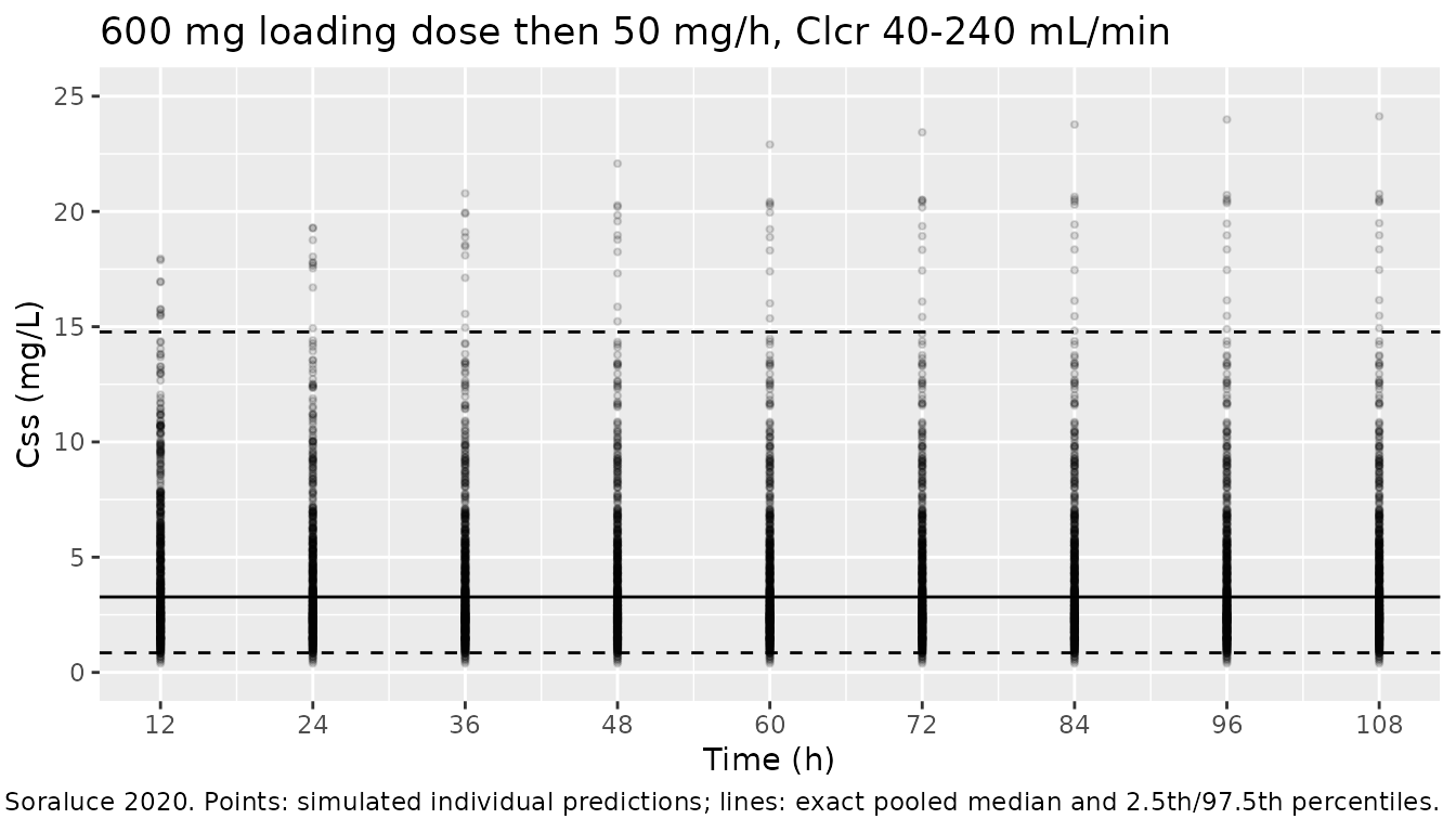
Table 4 - probability of target attainment at 600 mg every 12 h
Table 4 reports the share of the observed patients whose
measured concentrations met AUC24/MIC >= 80 and
100% T>MIC, which the model can only approximate: the
simulated cohort draws covariates from the Table 1 medians and ranges,
not from the 40 real patients, and the observed percentages come from 17
and 23 patients (one patient is 4-6 percentage points). The table is
therefore shown for context and not gated.
auc24 <- nca_res |>
  dplyr::filter(PPTESTCD == "auclast") |>
  dplyr::transmute(id, arm, auc24 = 2 * PPORRES)
cmin <- sim |>
  dplyr::filter(!is.na(Cc)) |>
  dplyr::group_by(id, arm) |>
  dplyr::summarise(cmin = min(Cc), .groups = "drop")

pta <- tidyr::expand_grid(MIC = c(1, 2, 4), arm = c("CRRT", "No CRRT")) |>
  dplyr::rowwise() |>
  dplyr::mutate(
    auc_sim = 100 * mean(auc24$auc24[auc24$arm == arm] / MIC >= 80),
    t_sim = 100 * mean(cmin$cmin[cmin$arm == arm] > MIC)
  ) |>
  dplyr::ungroup() |>
  dplyr::left_join(
    tibble::tribble(
      ~MIC, ~arm, ~auc_obs, ~t_obs,
      1, "CRRT", 96, 83,
      2, "CRRT", 52, 65,
      4, "CRRT", 0, 30,
      1, "No CRRT", 76, 76,
      2, "No CRRT", 65, 71,
      4, "No CRRT", 6, 29
    ),
    by = c("MIC", "arm")
  )

pta |>
  dplyr::mutate(dplyr::across(c(auc_sim, t_sim), round)) |>
  dplyr::select(arm, MIC, auc_sim, auc_obs, t_sim, t_obs) |>
  dplyr::rename(
    "Arm" = arm,
    "MIC (mg/L)" = MIC,
    "AUC24/MIC >= 80, simulated (%)" = auc_sim,
    "AUC24/MIC >= 80, Table 4 (%)" = auc_obs,
    "100% T>MIC, simulated (%)" = t_sim,
    "100% T>MIC, Table 4 (%)" = t_obs
  ) |>
knitr::kable(caption = "Target attainment at 600 mg q12h. Observed values from Table 4 of Soraluce 2020.")| Arm | MIC (mg/L) | AUC24/MIC >= 80, simulated (%) | AUC24/MIC >= 80, Table 4 (%) | 100% T>MIC, simulated (%) | 100% T>MIC, Table 4 (%) |
|---|---|---|---|---|---|
| CRRT | 1 | 95 | 96 | 82 | 83 |
| No CRRT | 1 | 72 | 76 | 54 | 76 |
| CRRT | 2 | 65 | 52 | 68 | 65 |
| No CRRT | 2 | 34 | 65 | 36 | 71 |
| CRRT | 4 | 24 | 0 | 48 | 30 |
| No CRRT | 4 | 6 | 6 | 20 | 29 |
The model agrees with the observed attainment at an MIC of 1 mg/L and
with the paper’s main conclusion that 600 mg every 12 h leaves many
patients below target at 2 and 4 mg/L. It does not reproduce the paper’s
finding of no difference between the arms. In the virtual cohort the
CRRT arm reaches the targets more often than the no-CRRT arm, because
its typical total clearance (2.62 + 4.35 * 6/44 + 2.51,
about 5.7 L/h) is well below that of the no-CRRT arm
(2.62 + 4.35 * 71.2/44, about 9.7 L/h): the extracorporeal
clearance replaces only part of the renal clearance lost with renal
failure. The observed no-CRRT patients reached the targets more often
than the virtual ones (65% vs about 35% at an MIC of 2 mg/L). The Table
4 percentages are computed from the measured concentrations of 17 and 23
real patients rather than from the model, so a mismatch of this size
does not by itself point to an error in the model file. The paper’s own
simulated checks (the Figure 3 inset above) are reproduced to within
1%.
Assumptions and deviations
- IIV scale. Table 3 prints the IIV as percentages without a formula. The model uses the log-normal CV reading, omega^2 = log(CV^2 + 1). The pooled simulated steady-state concentrations printed in the Figure 3 inset are reproduced to within 1% on this reading, while omega^2 = CV^2 misses the 97.5th percentile by 8% (and the 2.5th percentile by 8%).
- Residual error on the log scale. NONMEM was fitted to log-transformed concentrations with a combined error model. It is encoded here as additive (0.266 mg/L) plus proportional (0.159) on the linear concentration scale, the usual nlmixr2 equivalent. The two forms agree closely for concentrations well above the additive term, but they are not identical at low concentrations.
- Proportional error units. The Table 3 row reads ‘Residual error_proportional (%)’ with the value 0.159; it is taken as a fraction (15.9%), since 0.159% would be implausibly small for ICU data.
-
QEFF for non-CRRT subjects. The paper adds CLEC
“only for those undergoing CRRT”; the model has no separate indicator,
so
QEFFmust be set to 0 for subjects not on CRRT. -
CRCL normalisation.
CRCLis the raw urine-measured clearance in mL/min, not BSA-normalised. Supplying a Cockcroft-Gault estimate would be a change of assay; the Discussion attributes the strength of the covariate relationship in this cohort to the measured value. - Base-model value discrepancy. Results 3.1.2 gives the base-model IIV on CL as 98.7% and the Discussion as 97.8%; only the final model is packaged, so this has no effect.
-
Virtual cohort covariates. Only the median and
range of
CRCLand CLEC are published. The virtual cohort uses truncated log-normal distributions with the published medians, geometric SDs chosen by the maintainers so the draws span the published ranges; the Table 4 comparison depends on this choice and is not gated. - Unmodelled features. The Discussion reports a secondary peak 2-4 h after dose in about a third of patients, which the authors attributed to enterohepatic circulation but could not model; the packaged model, like the published one, does not reproduce it.