Acyclovir CNS distribution and dosing in viral encephalitis with Bayesian LeiCNS3.0 (Sun 2025)
Source:vignettes/articles/Sun_2025_acyclovir_pbpk.Rmd
Sun_2025_acyclovir_pbpk.RmdModel and source
Sun M, Manson ML, Martson A-G, Bodilsen J, de Lange ECM, Guo T. Revisiting acyclovir dosing for adult viral encephalitis using a full Bayesian LeiCNS PBPK modeling approach. Clin Pharmacokinet 2025;64(9):1413. doi:10.1007/s40262-025-01545-w.
The paper fits the human LeiCNS3.0 CNS physiologically-based PK model to aggregate plasma and lumbar CSF (subarachnoid space, SAS) acyclovir concentrations after oral valacyclovir, using full Bayesian estimation in Stan/Torsten. Eight sensitive parameters (plasma clearance, central volume, absorption rate, SAS volume, BBB pore size, BBB surface area, BBB width and CSF flow) were estimated with log-normal priors that represent an inflamed CNS. Everything else was fixed. The fitted model then simulates intravenous acyclovir regimens to compute the probability of reaching two efficacy targets (50%fT > IC50 and Cmin > IC50) in plasma, brain ECF and SAS, and a plasma peak toxicity threshold of 25 mg/L.
The CNS structure, the passive-transport regressions and the
asymmetry-factor closed forms are those of LeiCNS-PK3.0, Saleh et
al. 2021 (doi:10.1007/s10928-021-09768-7),
the paper’s reference [19]. The same structure ships in nlmixr2lib as
the mouse Saleh_2023_*_mouse_pbpk models.
mod <- readModelDb("Sun_2025_acyclovir_pbpk")How the pieces fit
-
Plasma is a one-compartment model with first-order
absorption. The absorption arm describes oral valacyclovir
(bioavailability 54.5%) and was used only for the fit. The paper’s
dosing simulations give acyclovir IV into
central. Plasma is a forcing function: CNS uptake does not deplete it. - CNS: brain microvasculature, brain ECF, a brain-cell-membrane (phospholipid) compartment, brain ICF, lysosomes, and the CSF chain lateral ventricle -> third + fourth ventricle -> cisterna magna -> SAS.
- Active transport is an efflux asymmetry factor on each barrier’s transcellular clearance, back-calculated so that the steady state honours Kp,uu,ECF = 0.32 and Kp,uu,CSF = 0.23 (Table S1). Acyclovir is very hydrophilic (logP -0.95), so the paracellular BBB clearance is about 125 times the transcellular one and the back-calculated BBB efflux factor is large.
-
BBB pore size (
PZ_BBB) is estimated in the paper but appears in no printed equation. Here it scales the paracellular BBB clearance linearly, relative to the healthy value of 0.0007 um (Table S2). See Assumptions and deviations. -
Residual error is log-normal for both fitted
endpoints, plasma (
Cc) and lumbar CSF (Cbrain_csf_sas). The brain ECF outputCbrain_ecfis a prediction only.
Population
The fitted data are mean concentrations digitised from two publications: Smith et al. 2010 (adults with normal renal function given valacyclovir 2000 mg QID; the chronic-kidney-disease arm was excluded) and Lycke et al. 2003 (adults with multiple sclerosis given valacyclovir 1000 mg TID). Endpoints are plasma and lumbar CSF. Only aggregate data were available, so the number of subjects is not reported and no interindividual variability was estimated (Discussion). The simulations target adults with HSV or VZV encephalitis. The paper’s priors represent this through a doubled SAS volume, a doubled BBB pore size and a tripled CSF flow (Table S2). The paper gives doses in mg/kg but does not report the body weight; this vignette uses 70 kg.
The paper’s simulation bands come from 500 posterior samples, not from virtual patients. The model file carries the posterior means. To show comparable bands, this vignette draws 200 parameter sets from independent log-normal distributions matched to the Table S3 posterior means and SDs. The posterior correlations are not reported.
Source trace
| Item | Value | Source |
|---|---|---|
| Plasma clearance CLe | 567 mL/min | Table S3 (posterior mean) |
| Central volume VCEN | 62481 mL | Table S3 |
| Absorption rate Ka (valacyclovir) | 0.0074 1/min | Table S3 |
| Bioavailability of valacyclovir F | 54.5% (fixed) | Table S1 |
| SAS volume VSAS | 278 mL | Table S3 |
| BBB pore size PZ_BBB | 0.00145 um | Table S3 |
| BBB surface area SA_BBB | 152997 cm^2 | Table S3 |
| BBB width W_BBB | 0.0000515 cm | Table S3 |
| CSF flow QCSF | 1.096 mL/min | Table S3 |
| Reference (healthy) BBB pore size | 0.0007 um | Table S2, ‘Healthy’ column |
| Residual SD plasma / SAS (log scale) | 0.301 / 0.137 | Table S3 (Sigma_Plasma, Sigma_SAS) |
| MW, logP, pKa, pKb | 225.2, -0.95, 11.98, 3.02 | Table S1 (DrugBank) |
| Kp,uu,ECF / Kp,uu,CSF | 0.32 / 0.23 | Table S1 |
| Brain volumes MV / ECF / ICF / LYS | 47 / 253 / 1000 / 12.5 mL | Table S1 |
| CSF volumes LV / TFV / CM | 20 / 3 / 1 mL | Table S1 |
| Brain phospholipid volume | 5% of 1250 mL | Saleh 2021; Vtot from Table S1 |
| Q_CBF / Q_ECF | 689 / 0.2 mL/min | Table S1 |
| SA BCSFB / BCM / LYS | 15000 / 2666520 / 1980260 cm^2 | Table S1 |
| Effective SA trans / para BBB / para BCSFB | 99.8% / 0.004% / 0.016% | Table S1 |
| BCSFB width | 0.5 um | Table S1 |
| pH plasma, MV / ECF / CSF / ICF / LYS | 7.4 / 7.3 / 7.3 / 7.0 / 5.0 | Table S1 |
| Unbound fraction in plasma | 1 (assumed) | Not reported; see Assumptions |
| Daq, P0 regressions | log10 Daq = -4.113 - 0.4609 log10 MW; log10 P0 = 0.939 logP - 6.21 | Saleh 2021 supplementary equations |
| Qp = Daq / width x SA x f_para; Qt = 0.5 P0 SA f_trans | - | Saleh 2021 supplementary equations |
| Qp_BBB x PZ_BBB / 0.0007 | - | Maintainers’ assumption (Figure S1 direction) |
| Efflux asymmetry factors (BBB, LV, TFV) | - | Saleh 2021 supplementary equations |
| Log-normal likelihood for plasma and SAS | - | Methods, ‘Defining Prior Distribution’ |
Simulation helpers
# Model time is minutes; doses are mg; concentrations are mg/L.
body_weight <- 70

# Both fitted endpoints are declared in the model, so observation rows name
# an ODE state and carry dvid = 1 (rxode2 returns every output column).
make_events <- function(n_id, amt, dur_min, ii_min, n_dose, cmt, obs_min) {
  dose <- expand.grid(time = (seq_len(n_dose) - 1) * ii_min, id = seq_len(n_id))
  dose$amt <- amt
  dose$evid <- 1L
  dose$cmt <- cmt
  dose$dvid <- NA_integer_
  dose$rate <- if (dur_min > 0) amt / dur_min else 0
  obs <- expand.grid(time = obs_min, id = seq_len(n_id))
  obs$amt <- 0
  obs$evid <- 0L
  obs$cmt <- "central"
  obs$dvid <- 1L
  obs$rate <- 0
  cols <- c("id", "time", "amt", "evid", "cmt", "dvid", "rate")
  ev <- rbind(dose[, cols], obs[, cols])
  ev[order(ev$id, ev$time, -ev$evid), ]
}

# The model has no random effects, so the per-draw parameter sets come in
# through `params`; rxode2's note that a multi-subject solve has no omega is
# expected and muffled.
muffle_no_omega <- function(w) {
  if (grepl("without 'omega'", conditionMessage(w), fixed = TRUE)) {
    invokeRestart("muffleWarning")
  }
}

solve_mod <- function(ev, params = NULL) {
  out <- withCallingHandlers(
    rxode2::rxSolve(
      mod,
      events = ev,
      params = params,
      useLinCmt = FALSE,
      returnType = "data.frame"
    ),
    warning = muffle_no_omega
  )
  out$time_h <- out$time / 60
  out
}

# Approximate posterior: independent log-normals matched to the Table S3
# means and SDs (the posterior correlations are not reported).
posterior <- tibble::tribble(
  ~param, ~mean, ~sd, ~log_param,
  "lcl", 567, 23, TRUE,
  "lvc", 62481, 12268, TRUE,
  "lka", 0.0074, 0.00139, TRUE,
  "V_SAS", 278, 63, FALSE,
  "PZ_BBB", 0.00145, 0.000359, FALSE,
  "SA_BBB", 152997, 36461, FALSE,
  "w_BBB", 0.0000515, 0.0000127, FALSE,
  "Q_CSF", 1.096, 0.238, FALSE
)

draw_posterior <- function(n, posterior) {
  out <- lapply(seq_len(nrow(posterior)), function(i) {
    sdlog <- sqrt(log(1 + (posterior$sd[i] / posterior$mean[i])^2))
    meanlog <- log(posterior$mean[i]) - sdlog^2 / 2
    x <- exp(stats::rnorm(n, meanlog, sdlog))
    if (posterior$log_param[i]) log(x) else x
  })
  names(out) <- posterior$param
  as.data.frame(out)
}

set.seed(2025)
rxode2::rxSetSeed(2025)
n_draw <- 200
draws <- draw_posterior(n_draw, posterior)
Structural checks
LeiCNS-PK3.0 back-calculates the asymmetry factors so that the steady state honours the Kp,uu values exactly. So under a constant plasma concentration, brain ECF/plasma must converge to Kp,uu,ECF = 0.32 and SAS/plasma to Kp,uu,CSF = 0.23 (unbound fraction 1). A one-compartment IV dosing interval at steady state must also give AUC = dose / CL.
# 7-day constant-rate infusion (100 mg/h) reaches steady state in every
# compartment (slowest relaxation: SAS turnover V_SAS / Q_CSF of about 4 h).
ev_inf <- make_events(1, 100 * 24 * 7, 7 * 24 * 60, 0, 1, "central", c(0, 7 * 24 * 60))
ss <- rxode2::rxSolve(mod, events = ev_inf, useLinCmt = FALSE, returnType = "data.frame",
                      rtol = 1e-10, atol = 1e-12, maxsteps = 1e6)
ss_end <- ss[ss$time == max(ss$time), ]
ss_ratio <- c(
  ecf = ss_end$Cbrain_ecf / ss_end$Cc,
  sas = ss_end$Cbrain_csf_sas / ss_end$Cc
)
ss_ratio
#>  ecf  sas
#> 0.32 0.23
stopifnot(
  abs(ss_ratio[["ecf"]] / 0.32 - 1) < 1e-4,
  abs(ss_ratio[["sas"]] / 0.23 - 1) < 1e-4
)
Replicate Figure 2: posterior predictive check against the fitted data
The fitted regimens are valacyclovir 1000 mg TID (Lycke 2003; Figure
2 shows 32-40 h) and 2000 mg QID (Smith 2010; Figure 2 shows 24-32 h
after the fifth dose). Doses are entered as valacyclovir mg into
depot, with F = 54.5%. The points are the published mean
observations, read by eye from Figure 2 by the maintainers and
approximate.
fig2_obs <- tibble::tribble(
  ~study, ~endpoint, ~time_h, ~conc,
  "Lycke 2003: 1000 mg TID", "Plasma", 32, 0.85,
  "Lycke 2003: 1000 mg TID", "Plasma", 33, 3.9,
  "Lycke 2003: 1000 mg TID", "Plasma", 33.5, 5.1,
  "Lycke 2003: 1000 mg TID", "Plasma", 34, 5.3,
  "Lycke 2003: 1000 mg TID", "Plasma", 34.5, 4.0,
  "Lycke 2003: 1000 mg TID", "Plasma", 35, 3.3,
  "Lycke 2003: 1000 mg TID", "Plasma", 40, 0.75,
  "Lycke 2003: 1000 mg TID", "SAS", 34, 0.52,
  "Lycke 2003: 1000 mg TID", "SAS", 40, 0.55,
  "Smith 2010: 2000 mg QID", "Plasma", 24, 4.1,
  "Smith 2010: 2000 mg QID", "Plasma", 24.5, 3.7,
  "Smith 2010: 2000 mg QID", "Plasma", 25, 4.4,
  "Smith 2010: 2000 mg QID", "Plasma", 25.5, 6.3,
  "Smith 2010: 2000 mg QID", "Plasma", 27, 8.4,
  "Smith 2010: 2000 mg QID", "Plasma", 28, 5.6,
  "Smith 2010: 2000 mg QID", "Plasma", 30, 3.2,
  "Smith 2010: 2000 mg QID", "Plasma", 32, 1.9,
  "Smith 2010: 2000 mg QID", "SAS", 24, 1.52,
  "Smith 2010: 2000 mg QID", "SAS", 24.5, 1.37,
  "Smith 2010: 2000 mg QID", "SAS", 25, 1.57,
  "Smith 2010: 2000 mg QID", "SAS", 25.5, 1.21,
  "Smith 2010: 2000 mg QID", "SAS", 27, 1.47,
  "Smith 2010: 2000 mg QID", "SAS", 28, 1.56,
  "Smith 2010: 2000 mg QID", "SAS", 30, 1.53,
  "Smith 2010: 2000 mg QID", "SAS", 32, 0.99
)

sim_lycke <- solve_mod(
  make_events(n_draw, 1000, 0, 8 * 60, 5, "depot", seq(32 * 60, 40 * 60, by = 10)),
  draws
)
sim_lycke$study <- "Lycke 2003: 1000 mg TID"
sim_smith <- solve_mod(
  make_events(n_draw, 2000, 0, 6 * 60, 5, "depot", seq(24 * 60, 32 * 60, by = 10)),
  draws
)
sim_smith$study <- "Smith 2010: 2000 mg QID"

fig2_sim <- bind_rows(sim_lycke, sim_smith) |>
  select(id, study, time_h, Plasma = Cc, SAS = Cbrain_csf_sas) |>
  pivot_longer(c(Plasma, SAS), names_to = "endpoint", values_to = "conc") |>
  group_by(study, endpoint, time_h) |>
  summarise(
    median = median(conc),
    lo = quantile(conc, 0.025),
    hi = quantile(conc, 0.975),
    .groups = "drop"
  )

ggplot(fig2_sim, aes(time_h)) +
  geom_ribbon(aes(ymin = lo, ymax = hi), fill = "darkseagreen", alpha = 0.4) +
  geom_line(aes(y = median)) +
  geom_point(data = fig2_obs, aes(y = conc), shape = 1) +
  facet_grid(endpoint ~ study, scales = "free") +
  labs(
    x = "Time (h)", y = "Acyclovir concentration (mg/L)",
    caption = "Replicates Figure 2 of Sun 2025 (band: 95% parameter-uncertainty interval)."
  )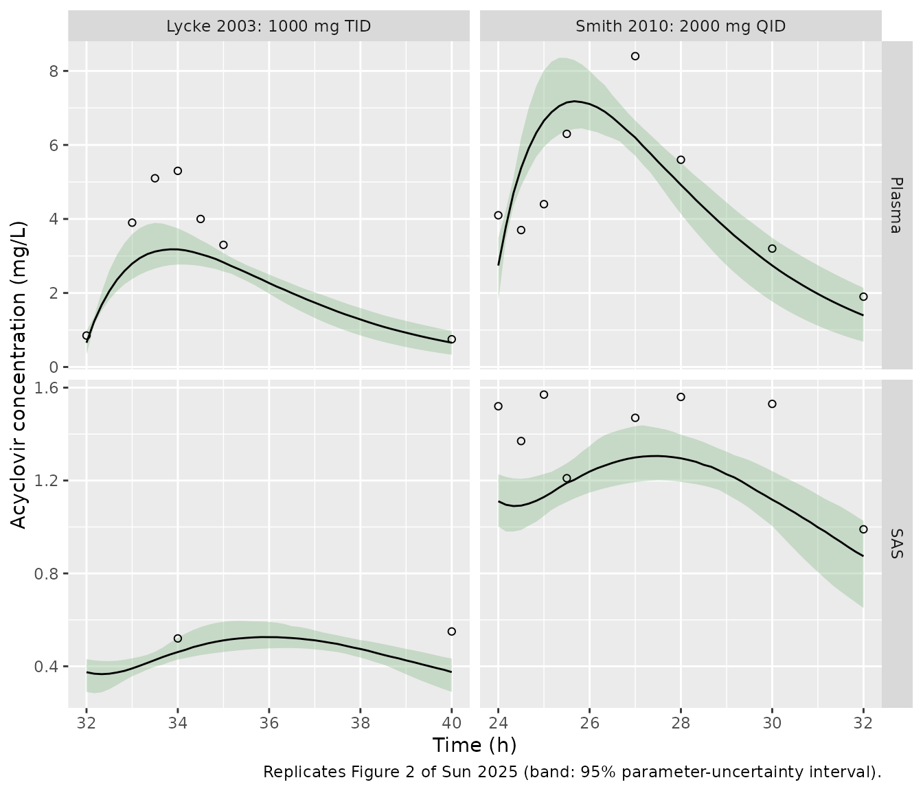
The simulated medians run about 20-25% below the published posterior predictive medians in both studies and in both matrices, for example a Lycke plasma peak of about 3.2 mg/L against about 4.2 mg/L in Figure 2. The dose is absolute here, so body weight cannot explain the gap. See Assumptions and deviations.
Replicate Figure 3: the standard regimen in plasma, brain ECF and SAS
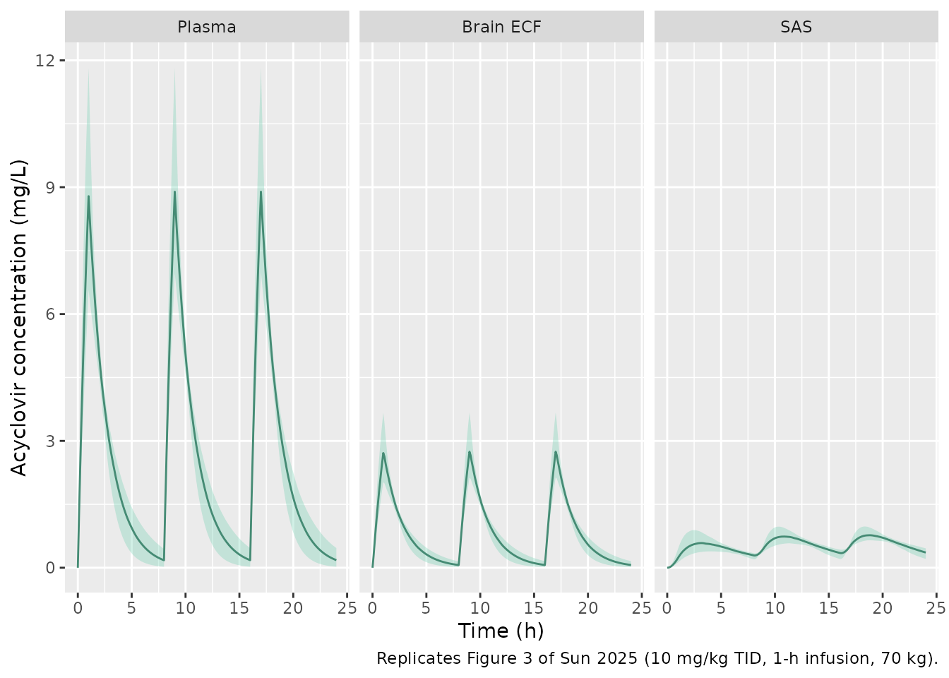
10 mg/kg (700 mg at 70 kg) IV every 8 h as a 1-h infusion, three doses.
dose_std <- 10 * body_weight
sim_std <- solve_mod(
  make_events(n_draw, dose_std, 60, 8 * 60, 3, "central", seq(0, 24 * 60, by = 6)),
  draws
)
fig3_long <- sim_std |>
  select(id, time_h, Plasma = Cc, `Brain ECF` = Cbrain_ecf, SAS = Cbrain_csf_sas) |>
  pivot_longer(-c(id, time_h), names_to = "compartment", values_to = "conc") |>
  mutate(compartment = factor(compartment, levels = c("Plasma", "Brain ECF", "SAS")))

fig3_long |>
  group_by(compartment, time_h) |>
  summarise(
    median = median(conc), lo = quantile(conc, 0.025), hi = quantile(conc, 0.975),
    .groups = "drop"
  ) |>
  ggplot(aes(time_h)) +
  geom_ribbon(aes(ymin = lo, ymax = hi), fill = "aquamarine3", alpha = 0.3) +
  geom_line(aes(y = median), colour = "aquamarine4") +
  facet_wrap(~compartment) +
  labs(
    x = "Time (h)", y = "Acyclovir concentration (mg/L)",
    caption = "Replicates Figure 3 of Sun 2025 (10 mg/kg TID, 1-h infusion, 70 kg)."
  )
PKNCA over the third dosing interval
nca_conc <- fig3_long |>
  filter(!is.na(conc)) |>
  mutate(
    compartment = as.character(compartment),
    conc = pmax(conc, 0),
    treatment = "10 mg/kg TID"
  )
nca_dose <- data.frame(
  id = rep(seq_len(n_draw), each = 3),
  time_h = rep(c(0, 8, 16), n_draw),
  amt = dose_std,
  treatment = "10 mg/kg TID"
)
nca_dose <- tidyr::crossing(nca_dose, compartment = c("Plasma", "Brain ECF", "SAS"))

conc_obj <- PKNCA::PKNCAconc(nca_conc, conc ~ time_h | treatment + compartment + id)
dose_obj <- PKNCA::PKNCAdose(nca_dose, amt ~ time_h | treatment + compartment + id)
intervals <- data.frame(
  start = 16, end = 24,
  auclast = TRUE, cmax = TRUE, cmin = TRUE, half.life = TRUE
)
nca_res <- PKNCA::pk.nca(PKNCA::PKNCAdata(conc_obj, dose_obj, intervals = intervals))

fig3_ref <- data.frame(
  compartment = c("Plasma", "Brain ECF", "SAS"),
  auclast = c(26.1, 17.1, 5.9),
  cmax = c(11.2, 6.6, 1.0),
  cmin = c(0.3, 0.2, 0.5),
  half.life = c(2.3, 2.4, 4.5)
)
nca_tab <- nlmixr2lib::ncaComparisonTable(
  nca_res, fig3_ref,
  by = "compartment",
  params = c("auclast", "cmax", "cmin", "half.life"),
  tolerance_pct = 20,
  units = c(auclast = "mg*h/L", cmax = "mg/L", cmin = "mg/L", half.life = "h")
)
knitr::kable(nca_tab, caption = "Third-interval (16-24 h) NCA: simulated median vs Figure 3 annotations.")| NCA parameter | compartment | Reference | Simulated | % diff |
|---|---|---|---|---|
| Cmax (mg/L) | Plasma | 11.2 | 8.89 | -20.6%* |
| Cmax (mg/L) | Brain ECF | 6.6 | 2.74 | -58.4%* |
| Cmax (mg/L) | SAS | 1 | 0.771 | -22.9%* |
| Cmin (mg/L) | Plasma | 0.3 | 0.179 | -40.4%* |
| Cmin (mg/L) | Brain ECF | 0.2 | 0.0648 | -67.6%* |
| Cmin (mg/L) | SAS | 0.5 | 0.346 | -30.9%* |
| AUClast (mg*h/L) | Plasma | 26.1 | 20.6 | -21.0%* |
| AUClast (mg*h/L) | Brain ECF | 17.1 | 6.6 | -61.4%* |
| AUClast (mg*h/L) | SAS | 5.9 | 4.68 | -20.8%* |
| t½ (h) | Plasma | 2.3 | 1.24 | -46.0%* |
| t½ (h) | Brain ECF | 2.4 | 1.29 | -46.2%* |
| t½ (h) | SAS | 4.5 | 3.54 | -21.2%* |
- differs from reference by more than ±20%.
per_id <- as.data.frame(nca_res$result) |>
  filter(PPTESTCD == "auclast") |>
  select(id, compartment, PPORRES) |>
  pivot_wider(names_from = compartment, values_from = PPORRES) |>
  mutate(
    cl_l_h = exp(draws$lcl[id]) * 60 / 1000,
    auc_closed = dose_std / cl_l_h,
    pct_diff = 100 * (Plasma / auc_closed - 1),
    ecf_ratio = `Brain ECF` / Plasma,
    sas_ratio = SAS / Plasma
  )
summary(per_id[, c("pct_diff", "ecf_ratio", "sas_ratio")])
#>     pct_diff          ecf_ratio      sas_ratio
#>  Min.   :-0.07673   Min.   :0.32   Min.   :0.2061
#>  1st Qu.:-0.02483   1st Qu.:0.32   1st Qu.:0.2264
#>  Median :-0.02031   Median :0.32   Median :0.2284
#>  Mean   :-0.02269   Mean   :0.32   Mean   :0.2271
#>  3rd Qu.:-0.01740   3rd Qu.:0.32   3rd Qu.:0.2295
#>  Max.   :-0.01594   Max.   :0.32   Max.   :0.2301
stopifnot(
  # Same parameters on both sides: only accumulation (< 0.1% after two
  # intervals at a 1.3-h half-life) and trapezoid error remain.
  abs(median(per_id$pct_diff)) < 2,
  quantile(abs(per_id$pct_diff), 0.9) < 5,
  # The printed asymmetry factors pin brain ECF / plasma to Kp,uu,ECF.
  abs(median(per_id$ecf_ratio) - 0.32) < 0.03,
  abs(median(per_id$sas_ratio) - 0.23) < 0.03
)
The plasma AUC matches dose/CL, and the brain ECF and SAS exposures sit at Kp,uu,ECF and Kp,uu,CSF times plasma. This is what the printed LeiCNS3.0 equations require. In Figure 3, SAS/plasma (5.9/26.1 = 0.23) agrees, but brain ECF/plasma is 17.1/26.1 = 0.66, about twice Kp,uu,ECF. The plasma AUC in Figure 3 (26.1 mg h/L) is also 1.27 times dose/CL at 70 kg. These are the starred rows above; they are not tuning targets. See Assumptions and deviations.
Replicate Figures 4 and 5: target attainment and peak toxicity
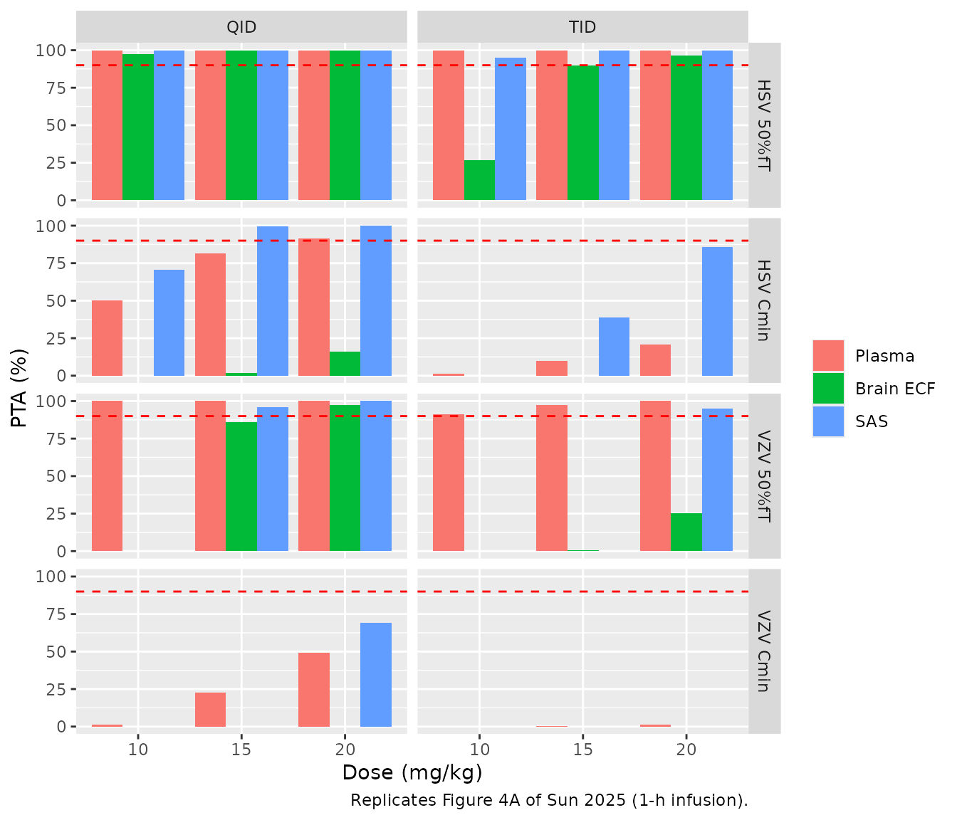
PTA is the percentage of the 200 posterior draws that meet a target on day 2 (24-48 h). The IC50 values are 0.56 mg/L (HSV) and 1.125 mg/L (VZV). 50%fT > IC50 requires the concentration to exceed IC50 for at least 12 of the 24 h. Cmin > IC50 requires the trough to exceed IC50 throughout.
regimens <- tidyr::crossing(
  dose_mgkg = c(10, 15, 20),
  freq = c("TID", "QID"),
  inf_h = 1
) |>
  bind_rows(tidyr::crossing(dose_mgkg = 20, freq = c("TID", "QID"), inf_h = c(1.5, 2))) |>
  mutate(regimen = sprintf("%d mg/kg %s, %.1f-h infusion", dose_mgkg, freq, inf_h))

simulate_regimen <- function(dose_mgkg, freq, inf_h, regimen) {
  ii <- if (freq == "TID") 8 * 60 else 6 * 60
  n_dose <- if (freq == "TID") 6 else 8
  ev <- make_events(n_draw, dose_mgkg * body_weight, inf_h * 60, ii, n_dose, "central",
                    seq(24 * 60, 48 * 60, by = 6))
  solve_mod(ev, draws) |>
    select(id, time_h, Plasma = Cc, `Brain ECF` = Cbrain_ecf, SAS = Cbrain_csf_sas) |>
    mutate(regimen = regimen, dose_mgkg = dose_mgkg, freq = freq, inf_h = inf_h)
}
sim_pta <- bind_rows(Map(
  simulate_regimen,
  regimens$dose_mgkg, regimens$freq, regimens$inf_h, regimens$regimen
)) |>
  pivot_longer(c(Plasma, `Brain ECF`, SAS), names_to = "compartment", values_to = "conc")

ic50 <- c(HSV = 0.56, VZV = 1.125)
per_draw <- sim_pta |>
  group_by(regimen, dose_mgkg, freq, inf_h, compartment, id) |>
  summarise(
    frac_hsv = mean(conc > ic50[["HSV"]]),
    frac_vzv = mean(conc > ic50[["VZV"]]),
    cmin = min(conc),
    cmax = max(conc),
    .groups = "drop"
  )
pta_tab <- per_draw |>
  group_by(regimen, dose_mgkg, freq, inf_h, compartment) |>
  summarise(
    `HSV 50%fT` = 100 * mean(frac_hsv >= 0.5),
    `HSV Cmin` = 100 * mean(cmin > ic50[["HSV"]]),
    `VZV 50%fT` = 100 * mean(frac_vzv >= 0.5),
    `VZV Cmin` = 100 * mean(cmin > ic50[["VZV"]]),
    .groups = "drop"
  )
pta_tab |>
  filter(inf_h == 1) |>
  arrange(freq, dose_mgkg, compartment) |>
  select(-dose_mgkg, -freq, -inf_h) |>
  dplyr::rename(Regimen = regimen, Compartment = compartment) |>
knitr::kable(digits = 0, caption = "PTA (%) on day 2 (replicates Figure 4A of Sun 2025).")| Regimen | Compartment | HSV 50%fT | HSV Cmin | VZV 50%fT | VZV Cmin |
|---|---|---|---|---|---|
| 10 mg/kg QID, 1.0-h infusion | Brain ECF | 98 | 0 | 0 | 0 |
| 10 mg/kg QID, 1.0-h infusion | Plasma | 100 | 50 | 100 | 2 |
| 10 mg/kg QID, 1.0-h infusion | SAS | 100 | 70 | 0 | 0 |
| 15 mg/kg QID, 1.0-h infusion | Brain ECF | 100 | 2 | 86 | 0 |
| 15 mg/kg QID, 1.0-h infusion | Plasma | 100 | 82 | 100 | 22 |
| 15 mg/kg QID, 1.0-h infusion | SAS | 100 | 100 | 96 | 0 |
| 20 mg/kg QID, 1.0-h infusion | Brain ECF | 100 | 16 | 98 | 0 |
| 20 mg/kg QID, 1.0-h infusion | Plasma | 100 | 92 | 100 | 49 |
| 20 mg/kg QID, 1.0-h infusion | SAS | 100 | 100 | 100 | 69 |
| 10 mg/kg TID, 1.0-h infusion | Brain ECF | 26 | 0 | 0 | 0 |
| 10 mg/kg TID, 1.0-h infusion | Plasma | 100 | 2 | 91 | 0 |
| 10 mg/kg TID, 1.0-h infusion | SAS | 95 | 0 | 0 | 0 |
| 15 mg/kg TID, 1.0-h infusion | Brain ECF | 90 | 0 | 0 | 0 |
| 15 mg/kg TID, 1.0-h infusion | Plasma | 100 | 10 | 98 | 0 |
| 15 mg/kg TID, 1.0-h infusion | SAS | 100 | 39 | 0 | 0 |
| 20 mg/kg TID, 1.0-h infusion | Brain ECF | 96 | 0 | 26 | 0 |
| 20 mg/kg TID, 1.0-h infusion | Plasma | 100 | 21 | 100 | 2 |
| 20 mg/kg TID, 1.0-h infusion | SAS | 100 | 86 | 95 | 0 |
pta_tab |>
  filter(inf_h == 1) |>
  pivot_longer(c(`HSV 50%fT`, `HSV Cmin`, `VZV 50%fT`, `VZV Cmin`), names_to = "target", values_to = "pta") |>
  mutate(compartment = factor(compartment, levels = c("Plasma", "Brain ECF", "SAS"))) |>
  ggplot(aes(factor(dose_mgkg), pta, fill = compartment)) +
  geom_col(position = "dodge") +
  geom_hline(yintercept = 90, linetype = "dashed", colour = "red") +
  facet_grid(target ~ freq) +
  labs(
    x = "Dose (mg/kg)", y = "PTA (%)", fill = NULL,
    caption = "Replicates Figure 4A of Sun 2025 (1-h infusion)."
  )
tox_tab <- per_draw |>
  filter(compartment == "Plasma", dose_mgkg >= 15) |>
  group_by(regimen) |>
  summarise(
    `Median plasma Cmax (mg/L)` = median(cmax),
    `97.5th percentile (mg/L)` = quantile(cmax, 0.975),
    `% above 25 mg/L` = 100 * mean(cmax > 25),
    .groups = "drop"
  ) |>
  dplyr::rename(Regimen = regimen)
knitr::kable(tox_tab, digits = 1,
caption = "Day-2 plasma peaks against the 25 mg/L threshold (replicates Figures 4B and 5B of Sun 2025).")| Regimen | Median plasma Cmax (mg/L) | 97.5th percentile (mg/L) | % above 25 mg/L |
|---|---|---|---|
| 15 mg/kg QID, 1.0-h infusion | 13.6 | 17.8 | 0.0 |
| 15 mg/kg TID, 1.0-h infusion | 13.3 | 17.7 | 0.0 |
| 20 mg/kg QID, 1.0-h infusion | 18.2 | 23.8 | 0.5 |
| 20 mg/kg QID, 1.5-h infusion | 16.1 | 19.7 | 0.0 |
| 20 mg/kg QID, 2.0-h infusion | 14.3 | 16.5 | 0.0 |
| 20 mg/kg TID, 1.0-h infusion | 17.8 | 23.7 | 0.5 |
| 20 mg/kg TID, 1.5-h infusion | 15.7 | 19.6 | 0.0 |
| 20 mg/kg TID, 2.0-h infusion | 14.0 | 16.5 | 0.0 |
pta_tab |>
  filter(dose_mgkg == 20) |>
  arrange(freq, inf_h, compartment) |>
  select(-dose_mgkg, -freq, -inf_h) |>
  dplyr::rename(Regimen = regimen, Compartment = compartment) |>
knitr::kable(digits = 0, caption = "PTA (%) at 20 mg/kg by infusion duration (replicates Figure 5A of Sun 2025).")| Regimen | Compartment | HSV 50%fT | HSV Cmin | VZV 50%fT | VZV Cmin |
|---|---|---|---|---|---|
| 20 mg/kg QID, 1.0-h infusion | Brain ECF | 100 | 16 | 98 | 0 |
| 20 mg/kg QID, 1.0-h infusion | Plasma | 100 | 92 | 100 | 49 |
| 20 mg/kg QID, 1.0-h infusion | SAS | 100 | 100 | 100 | 69 |
| 20 mg/kg QID, 1.5-h infusion | Brain ECF | 100 | 26 | 100 | 0 |
| 20 mg/kg QID, 1.5-h infusion | Plasma | 100 | 94 | 100 | 66 |
| 20 mg/kg QID, 1.5-h infusion | SAS | 100 | 100 | 100 | 80 |
| 20 mg/kg QID, 2.0-h infusion | Brain ECF | 100 | 42 | 100 | 0 |
| 20 mg/kg QID, 2.0-h infusion | Plasma | 100 | 96 | 100 | 80 |
| 20 mg/kg QID, 2.0-h infusion | SAS | 100 | 100 | 100 | 88 |
| 20 mg/kg TID, 1.0-h infusion | Brain ECF | 96 | 0 | 26 | 0 |
| 20 mg/kg TID, 1.0-h infusion | Plasma | 100 | 21 | 100 | 2 |
| 20 mg/kg TID, 1.0-h infusion | SAS | 100 | 86 | 95 | 0 |
| 20 mg/kg TID, 1.5-h infusion | Brain ECF | 100 | 0 | 42 | 0 |
| 20 mg/kg TID, 1.5-h infusion | Plasma | 100 | 30 | 100 | 2 |
| 20 mg/kg TID, 1.5-h infusion | SAS | 100 | 90 | 92 | 0 |
| 20 mg/kg TID, 2.0-h infusion | Brain ECF | 100 | 0 | 72 | 0 |
| 20 mg/kg TID, 2.0-h infusion | Plasma | 100 | 42 | 100 | 3 |
| 20 mg/kg TID, 2.0-h infusion | SAS | 100 | 95 | 90 | 0 |
Against the paper’s findings:
- Reproduced: the standard 10 mg/kg TID regimen fails Cmin > IC50 in every compartment for both viruses, and 20 mg/kg TID still fails it for VZV. Moving to QID raises Cmin attainment more than raising the dose does (10 mg/kg QID beats 20 mg/kg TID in plasma). SAS has the highest troughs and brain ECF the lowest. Extending the infusion to 1.5 or 2 h lowers the plasma peak without losing attainment at 20 mg/kg; here it raises Cmin attainment, where the paper reports it as comparable.
- Not reproduced: brain ECF sits at 0.32 times plasma here, not at about 0.66 as in Figure 3, so brain ECF attainment is far below Figure 4A. At 10 mg/kg TID, HSV 50%fT > IC50 fails in brain ECF here, while the paper reports at least 90% in every compartment. Cmin > IC50 in brain ECF stays low even at QID. Plasma and SAS also run about 20% lower than in the paper, so attainment there is somewhat lower too. 20 mg/kg does not cross 25 mg/L in plasma here, while Figure 4B shows it does in the paper. The dose recommendations of the paper therefore rest on the published simulations and cannot be re-derived from this model as printed.
Assumptions and deviations
The published simulations cannot be fully reproduced from what the
paper prints. The authors’ Stan/Torsten code is available from them on
request and is not deposited. The authors’ public
LeiCNS-Source repository holds parameter tables only. The
model file follows the printed LeiCNS-PK3.0 equations with the Table S1
and S3 values. The gaps:
-
BBB pore size has no printed equation.
PZ_BBBis one of the eight estimated parameters (0.00145 um), but the LeiCNS-PK3.0 paracellular clearanceQp = Daq / width x SAcontains no pore term. In Figure S1, pore size changes exposure in the same direction as BBB surface area. The model therefore multiplies the paracellular BBB clearance byPZ_BBB / 0.0007, the healthy value in Table S2. This form is the maintainers’ assumption. It affects only the BBB clearance magnitudes, because the asymmetry factors are back-calculated with the same clearances. - Brain ECF exposure is about half of Figure 3. With the printed asymmetry-factor closed forms, brain ECF/plasma is pinned to Kp,uu,ECF = 0.32 whatever the other parameters are (structural checks above). Figure 3 shows 17.1/26.1 = 0.66 for AUC and 6.6/11.2 = 0.59 for Cmax. The asymmetry factor printed for acyclovir is large (BBB paracellular clearance far exceeds transcellular), so the published curves probably used asymmetry factors computed differently from the printed closed forms (for example, at healthy physiology rather than at the posterior). The source does not say which, so the model keeps the printed forms. SAS agrees with Kp,uu,CSF.
- Plasma exposure is about 1.25-1.3 times higher in every published simulation. This holds for the oral fits in Figure 2 (absolute doses) as well as the IV mg/kg simulations in Figures 3, 4B and 5B. The Figure 3 plasma AUC of 26.1 mg h/L at 700 mg corresponds to a clearance of about 26.8 L/h (447 mL/min), against the Table S3 posterior mean of 567 mL/min (34.0 L/h). Body weight for the mg/kg doses is not reported; 70 kg is used. The Figure 3 annotation ‘t1/2 2.3 h’ also differs from the plotted plasma decay and from CL/V (about 1.3 h). The model keeps the Table S3 values.
- Unbound fraction in plasma = 1. Table S1 lists no plasma protein binding. The SAS/plasma ratio in Figure 3 (0.23) equals Kp,uu,CSF only if the CNS is driven by the total plasma concentration.
- One Kp,uu,CSF for both CSF sites. The asymmetry-factor closed forms need Kp,uu at the lateral ventricle and at the cisterna magna. Both take the single reported Kp,uu,CSF = 0.23.
- Brain phospholipid volume is 5% of the 1250 mL total brain volume, as in Saleh 2021. Sun 2025 does not list it.
- Oral dose units. Table S1 labels F = 54.5% the ‘bioavailability of valacyclovir’, so oral doses are entered as valacyclovir mg. Entering acyclovir-equivalent mg (x 225.2/324.3) would lower the Figure 2 predictions by a further 31%.
- Parameter uncertainty in this vignette comes from independent log-normals matched to the Table S3 posterior means and SDs, because the posterior correlations are not reported. The paper used 500 joint posterior samples. The model file carries the posterior means as typical values and has no interindividual variability, as in the paper.
- Physiology. Table S1 lists the brain microvasculature volume as 47 mL (Saleh 2021 lists 45 mL); the model uses 47 mL. The BCSFB pore size (0.027 um, Table S1) is at its healthy value, so it does not alter the BCSFB paracellular clearance.