Eribulin CRPC PSA disease-progression model (van Hasselt 2015)
Source:vignettes/articles/vanHasselt_2015_eribulin.Rmd
vanHasselt_2015_eribulin.RmdModel and source
- Citation: van Hasselt JGC, Gupta A, Hussein Z, Beijnen JH, Schellens JHM, Huitema ADR. Disease Progression/Clinical Outcome Model for Castration-Resistant Prostate Cancer in Patients Treated With Eribulin. CPT Pharmacometrics Syst Pharmacol. 2015;4(7):386-395. doi:[10.1002/psp4.49](https://doi.org/10.1002/psp4.49).
- Article (open access): https://doi.org/10.1002/psp4.49
This vignette validates the disease-progression (DP) sub-model from
van Hasselt 2015, which describes prostate-specific antigen (PSA)
dynamics in metastatic castration-resistant prostate cancer (mCRPC)
patients on eribulin mesilate using a K-PD framework. The paper’s
companion parametric Weibull survival sub-model (clinical outcome) is
fit in R survreg, not in NONMEM, and is not encoded here – it is a
covariate regression on individual-predicted DP-model summaries (time to
PSA nadir, baseline PSA, PSA growth rate, ECOG score) rather than an ODE
structure, and so falls outside the scope of an nlmixr2 / rxode2 model.
The DP sub-model alone is what vanHasselt_2015_eribulin
packages.
Population
108 men with metastatic castration-resistant prostate cancer from a single Phase II clinical trial of eribulin mesilate (de Bono et al. Ann Oncol 2012;23:1241; the modelling paper’s reference 33). The cohort was stratified by prior taxane therapy: 50 patients had received prior docetaxel and 58 were taxane-naive. Eribulin was administered IV per the trial protocol; no PK samples were collected, so individual per-dose AUC values used as the DP-model input were predicted using an upstream eribulin population PK model (3-compartment linear elimination with albumin / alkaline phosphatase / total bilirubin on clearance; Majid et al. J Clin Pharmacol 2014;54:1134; van Hasselt et al. Br J Clin Pharmacol 2013;76:412 – referenced but not encoded here). PSA-time profiles were analysed in NONMEM 7.2 using first-order conditional estimation; survival was analysed separately in R survreg.
The same information is available programmatically via
readModelDb("vanHasselt_2015_eribulin")$population.
Source trace
Equations from van Hasselt 2015 Methods Eq. 1 (K-PD depot decay), Eq. 2 (PSA turnover with drug inhibition and resistance), and Eq. 4 (continuous covariate power form). Parameter values from Table 2 (final-model column).
| Equation / parameter | Value | Source location |
|---|---|---|
d/dt(depot_kpd) = -KP * depot_kpd, AUC bolus at dose
events |
n/a | Methods Eq. 1 |
d/dt(PSA) = PSA * (KG - KD0 * exp(-k_res*t) * depot_kpd) |
n/a | Methods Eq. 2 |
PSA(0) = PSA0 |
n/a | Methods Eq. 2 |
Covariate form (1 + NTRT/720)^h_NTRT on KD0 |
n/a | Methods Eq. 4; Table 2 footnote |
lkel |
fixed(log(6000)) |
Table 2: hKP = 6000 /day, fixed (Results: “We selected a large value of 6,000 to allow for a nearly instantaneous dosing event.”) |
lkd0 |
log(0.241) |
Table 2: hKD0 = 0.241 (RSE 32.6%) |
lkres |
log(0.0113) |
Table 2: hk = 0.0113 /day (RSE 44.3%) |
lkg |
log(0.00879) |
Table 2: hKG = 0.00879 /day (RSE 12.6%) |
lpsa0 |
log(23.2) |
Table 2: hPSA0 = 23.2 ng/mL (RSE 16.5%) |
e_prior_taxane_psa0 |
3.23 |
Table 2: hPSA0-PTAX = 3.23 (RSE 27.6%) |
e_prior_taxane_days_kd0 |
-4.00 |
Table 2: hKD0-NTRT = -4.00 (RSE 52.5%) |
var(etalkd0) |
0.96334 = log(1 + 1.273^2) |
Table 2: xKD0 = 127.3 CV% (RSE 14%, shrinkage 26%) |
var(etalkres) |
0.57665 = log(1 + 0.883^2) |
Table 2: xk = 88.3 CV% (RSE 37.5%, shrinkage 40%) |
var(etalkg) |
0.25342 = log(1 + 0.537^2) |
Table 2: xKG = 53.7 CV% (RSE 13.5%, shrinkage 18%) |
var(etalpsa0) |
0.99340 = log(1 + 1.304^2) |
Table 2: xPSA0 = 130.4 CV% (RSE 8.8%, shrinkage 1.0%) |
Correlation xk *xKD0
|
0.802 |
Table 2 footnote a |
Correlation xKG*xKD0
|
-0.293 |
Table 2 footnote b |
Correlation xKG*xk
|
-0.111 |
Table 2 footnote b |
Correlation xPSA0*xk
|
-0.094 |
Table 2 footnote c |
Correlation xPSA0*xKG
|
-0.032 |
Table 2 footnote c |
Correlation xPSA0*xKD0
|
0 (fixed) |
Results “Statistical model”: “the correlation between the drug effect parameter KD and PSA0, which approached zero in the final obtained estimate.” |
propSd |
0.342 |
Table 2: rprop = 34.2 CV% (RSE 27.5%, shrinkage 14%) |
| Typical per-dose eribulin AUC | 200 ng*h/mL |
Approximation for 1.4 mg/m^2 IV eribulin from the upstream popPK literature; the modelling paper does not tabulate individual AUC values in the on-disk text (Supporting Table S1 is referenced but not on disk). Used for the vignette demonstrations only; users with patient-specific AUC values should supply them per dose event. |
Virtual cohort and dosing schedule
The de Bono 2012 trial administered eribulin mesilate at 1.4 mg/m^2 IV on Day 1 and Day 8 of a 21-day cycle. The virtual cohort below uses four cycles (8 doses over the first 70 days) with a per-dose AUC of 200 ngh/mL supplied as the K-PD bolus, and follows PSA out to 200 days so the post-treatment regrowth phase is visible. The 200 ngh/mL placeholder is a literature-typical eribulin AUC for adults receiving the 1.4 mg/m^2 IV dose – the modelling paper does not publish individual AUC values in the main text on disk, so users with patient-level AUC predictions should override this default.
set.seed(2015)

n_subjects <- 100L
auc_per_dose <- 200          # ng*h/mL per dose
followup_days <- 200L
obs_times <- seq(0, followup_days, by = 7)

# Standard eribulin schedule: D1, D8 of each 21-day cycle.
cycles <- 4L
dose_times <- as.vector(outer(c(0, 7), 21 * (0:(cycles - 1)), `+`))
dose_times <- sort(dose_times)

# Per-subject baseline covariates (PRIOR_TAXANE roughly 50/50 split per the
# de Bono 2012 trial design; PRIOR_TAXANE_DAYS = 0 for the taxane-naive arm
# and a lognormal centred at the 720-day median for the prior-taxane arm).
subj <- tibble(
  id = seq_len(n_subjects),
  PRIOR_TAXANE = as.integer(seq_len(n_subjects) %% 2 == 0),
  PRIOR_TAXANE_DAYS = ifelse(
    seq_len(n_subjects) %% 2 == 0,
    pmin(rlnorm(n_subjects, meanlog = log(720), sdlog = 0.5), 1800),
    0
  )
)

# Dosing rows -- one per dose event, AUC supplied as amt into the depot_kpd
# K-PD compartment. evid = 1 is a bolus dose; cmt = "depot_kpd" routes the AUC
# into the drug-effect compartment.
dose_rows <- subj |>
  tidyr::crossing(time = dose_times) |>
  mutate(evid = 1L, amt = auc_per_dose, cmt = "depot_kpd")

# Observation rows (PSA samples) -- no dose, amt = 0.
obs_rows <- subj |>
  tidyr::crossing(time = obs_times) |>
  mutate(evid = 0L, amt = 0, cmt = NA_character_)

events <- bind_rows(dose_rows, obs_rows) |>
  arrange(id, time, desc(evid))

stopifnot(!anyDuplicated(unique(events[, c("id", "time", "evid")])))
Typical-value PSA trajectory (Figure 2 analogue)
van Hasselt 2015 Figure 2 plots individual log-PSA trajectories under
eribulin treatment. A typical-value simulation (zeroRe()
zeroes all between-subject random effects) shows the qualitative shape:
initial PSA decline driven by drug inhibition KD0 * D(t),
with the inhibition strength decaying over time via the resistance term
exp(-k_res*t), and underlying first-order growth at rate
KG that eventually dominates as resistance builds. The
right panel shows the same trajectory plotted on a log scale to match
Figure 2 of the paper.
mod <- readModelDb("vanHasselt_2015_eribulin")
mod_typ <- mod |> rxode2::zeroRe()

events_typ <- bind_rows(
  tibble(id = 1L, time = dose_times, evid = 1L, amt = auc_per_dose, cmt = "depot_kpd"),
  tibble(id = 1L, time = obs_times,  evid = 0L, amt = 0,           cmt = NA_character_)
) |>
  mutate(PRIOR_TAXANE = 0L, PRIOR_TAXANE_DAYS = 0) |>
  arrange(time, desc(evid))

sim_typ <- rxode2::rxSolve(mod_typ, events = events_typ) |> as.data.frame()
#> ℹ omega/sigma items treated as zero: 'etalpsa0', 'etalkg', 'etalkres', 'etalkd0'

ggplot(sim_typ, aes(time, PSA)) +
  geom_line(linewidth = 1, colour = "steelblue4") +
  geom_vline(xintercept = dose_times, linetype = "dotted", colour = "grey60") +
  labs(x = "Time (days)", y = "PSA (ng/mL)",
       title = "Typical taxane-naive patient on 4 cycles of eribulin",
       caption = "Replicates Figure 2 of van Hasselt 2015 (qualitative shape; vertical lines = dose events).") +
  theme_minimal()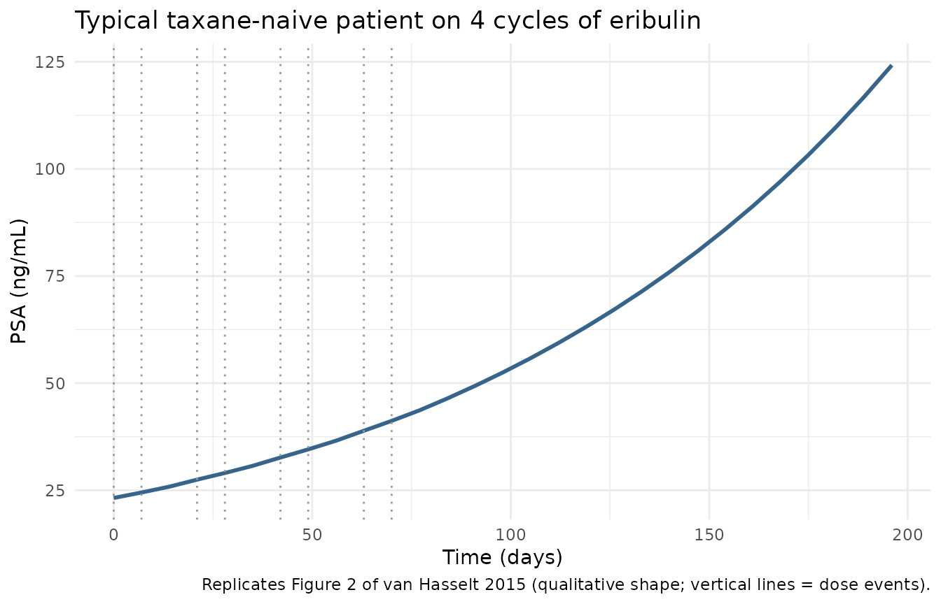
ggplot(sim_typ, aes(time, PSA)) +
  geom_line(linewidth = 1, colour = "steelblue4") +
  geom_vline(xintercept = dose_times, linetype = "dotted", colour = "grey60") +
  scale_y_log10() +
  labs(x = "Time (days)", y = "PSA (ng/mL, log scale)",
       title = "Same trajectory on log-PSA scale (matches Figure 2 axis)",
       caption = "Replicates Figure 2 of van Hasselt 2015.") +
  theme_minimal()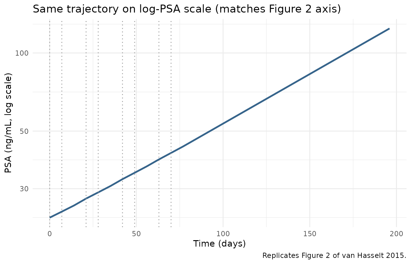
Covariate effects
Binary PRIOR_TAXANE on baseline PSA0
PRIOR_TAXANE = 1 (prior docetaxel pretreatment)
multiplies the typical baseline PSA0 by
e_prior_taxane_psa0 = 3.23, reflecting that
taxane-pretreated CRPC patients have more advanced disease at study
entry. The two panels below plot the typical-value PSA trajectory for a
taxane-naive vs prior-taxane patient with otherwise identical covariates
(PRIOR_TAXANE_DAYS = 0 is held in both for clarity).
ptax_events <- bind_rows(
  events_typ |> mutate(PRIOR_TAXANE = 0L, group = "Taxane-naive"),
  events_typ |> mutate(PRIOR_TAXANE = 1L, group = "Prior taxane")
) |>
  group_by(group) |>
  mutate(id = cur_group_id()) |>
  ungroup()

sim_ptax <- rxode2::rxSolve(
  mod_typ,
  events = ptax_events,
  keep   = "group"
) |> as.data.frame()
#> ℹ omega/sigma items treated as zero: 'etalpsa0', 'etalkg', 'etalkres', 'etalkd0'
#> Warning: multi-subject simulation without without 'omega'

ggplot(sim_ptax, aes(time, PSA, colour = group)) +
  geom_line(linewidth = 1) +
  geom_vline(xintercept = dose_times, linetype = "dotted", colour = "grey60") +
  labs(x = "Time (days)", y = "PSA (ng/mL)", colour = NULL,
       title = "Effect of PRIOR_TAXANE on PSA trajectory",
       caption = "Prior-taxane baseline PSA0 = 23.2 x 3.23 = 74.94 ng/mL (van Hasselt 2015 Table 2).") +
  theme_minimal()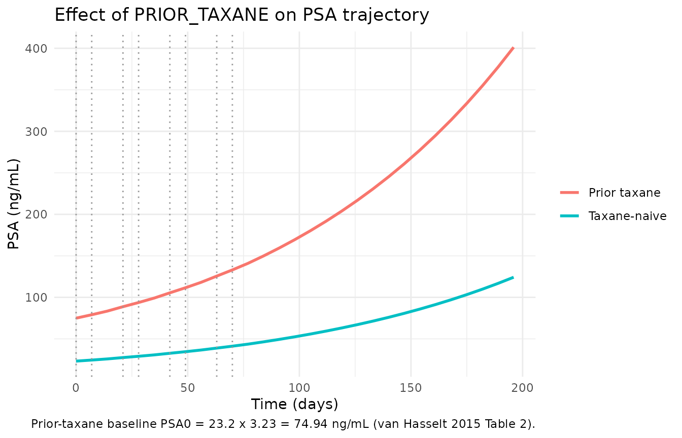
# Verify the baseline ratio at t = 0
psa_at_t0 <- sim_ptax |>
  filter(time == 0) |>
  select(group, PSA0_pred = PSA)

knitr::kable(psa_at_t0, digits = 3, caption = "Predicted PSA0 at t = 0 by prior-taxane status.")| group | PSA0_pred |
|---|---|
| Taxane-naive | 23.200 |
| Prior taxane | 74.936 |
Continuous PRIOR_TAXANE_DAYS on KD0
PRIOR_TAXANE_DAYS enters KD0 via van Hasselt 2015 Eq. 4:
KD0 = hKD0 * (1 + NTRT/720)^h_NTRT with
h_NTRT = -4.00. Patients with longer prior-taxane exposure
have lower drug-inhibition rate KD0 (cross-resistance between docetaxel
and eribulin via the shared microtubule-inhibition mechanism). The
(1 + NTRT/720) form is well-defined at
NTRT = 0 (collapses to 1), so the same equation applies
uniformly to taxane-naive and taxane-pretreated subjects.
ntrt_grid <- c(0, 360, 720, 1440)
ntrt_events <- purrr::map_dfr(seq_along(ntrt_grid), function(i) {
  events_typ |>
    mutate(
      PRIOR_TAXANE      = as.integer(ntrt_grid[i] > 0),
      PRIOR_TAXANE_DAYS = ntrt_grid[i],
      ntrt_label        = sprintf("NTRT = %d days", ntrt_grid[i]),
      id                = i
    )
})

sim_ntrt <- rxode2::rxSolve(
  mod_typ,
  events = ntrt_events,
  keep   = "ntrt_label"
) |> as.data.frame()
#> ℹ omega/sigma items treated as zero: 'etalpsa0', 'etalkg', 'etalkres', 'etalkd0'
#> Warning: multi-subject simulation without without 'omega'

ggplot(sim_ntrt, aes(time, PSA, colour = ntrt_label)) +
  geom_line(linewidth = 1) +
  geom_vline(xintercept = dose_times, linetype = "dotted", colour = "grey60") +
  labs(x = "Time (days)", y = "PSA (ng/mL)", colour = NULL,
       title = "Effect of PRIOR_TAXANE_DAYS on PSA inhibition",
       caption = "Longer prior taxane shrinks KD0 = 0.241 x (1 + NTRT/720)^-4, weakening eribulin's PSA inhibition.") +
  theme_minimal()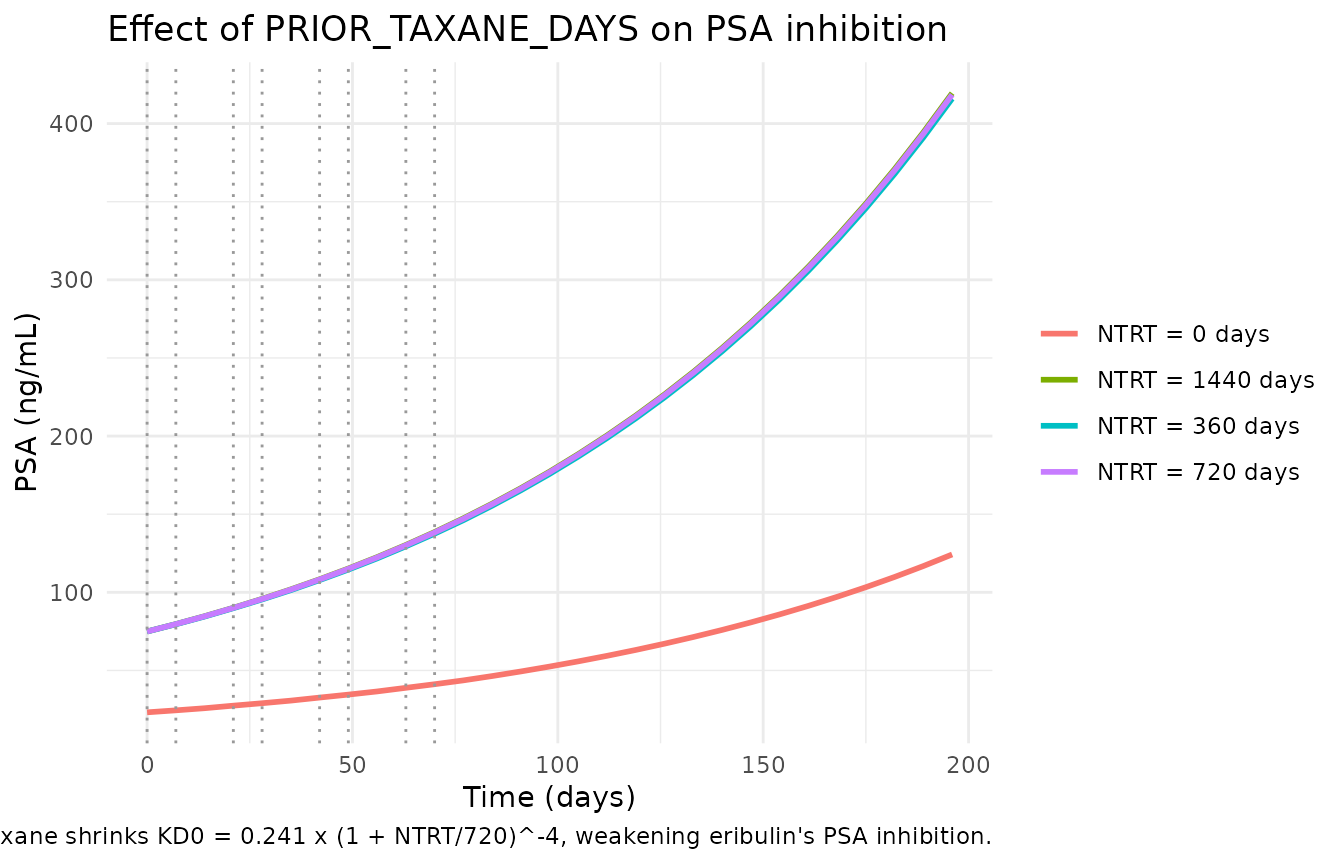
# Quantify the KD0 multiplier for each NTRT value
kd0_multiplier <- tibble(
  NTRT_days = ntrt_grid,
  multiplier = (1 + ntrt_grid / 720)^(-4),
  KD0_effective = 0.241 * multiplier
)

knitr::kable(
  kd0_multiplier, digits = 4,
  caption = "Effective KD0 by prior-taxane duration. The (1 + NTRT/720)^-4 form gives 1 at NTRT = 0 (taxane-naive), 0.0625 at NTRT = 720 (the population median), and 0.0123 at NTRT = 1440 (heavy pretreatment)."
)| NTRT_days | multiplier | KD0_effective |
|---|---|---|
| 0 | 1.0000 | 0.2410 |
| 360 | 0.1975 | 0.0476 |
| 720 | 0.0625 | 0.0151 |
| 1440 | 0.0123 | 0.0030 |
Stochastic VPC
Including the correlated lognormal IIV on KD0, k_res, KG, and PSA0 (paper Table 2; the KD0-vs-PSA0 covariance is fixed at zero) and the 34.2 CV% proportional residual error, the stochastic VPC across the 100-subject virtual cohort gives the percentile bands of PSA over time.
sim_iiv <- rxode2::rxSolve(
  mod,
  events = events,
  keep   = c("PRIOR_TAXANE")
) |> as.data.frame()

vpc <- sim_iiv |>
  group_by(time) |>
  summarise(
    Q05 = quantile(PSA, 0.05, na.rm = TRUE),
    Q50 = quantile(PSA, 0.50, na.rm = TRUE),
    Q95 = quantile(PSA, 0.95, na.rm = TRUE),
    .groups = "drop"
  )

ggplot(vpc, aes(time, Q50)) +
  geom_ribbon(aes(ymin = pmax(Q05, 0), ymax = Q95), alpha = 0.25, fill = "steelblue") +
  geom_line(linewidth = 1, colour = "steelblue4") +
  geom_vline(xintercept = dose_times, linetype = "dotted", colour = "grey60") +
  scale_y_log10() +
  labs(x = "Time (days)", y = "PSA (ng/mL, log scale)",
       title = "Stochastic VPC: median, 5/95 percentile bands",
       caption = "100 virtual subjects, 50/50 PRIOR_TAXANE split, correlated IIV per van Hasselt 2015 Table 2.") +
  theme_minimal()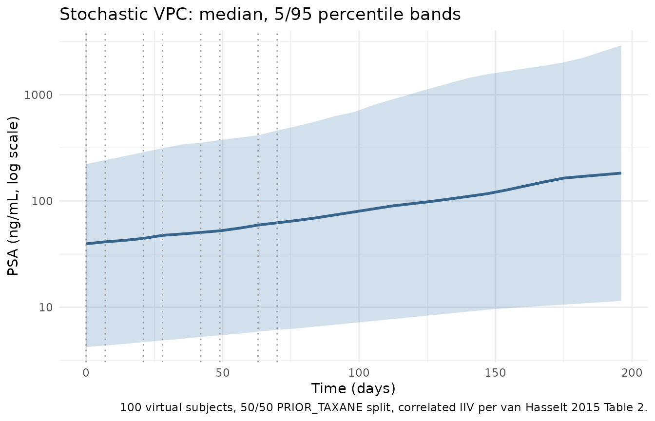
Mechanistic sanity checks
1. Drug-free trajectory = pure exponential growth at rate KG
With no doses, Eq. 2 reduces to dPSA/dt = KG * PSA, so
PSA grows exponentially with rate constant KG = 0.00879 /day (doubling
time = log(2) / KG = 78.9 days).
events_off <- tibble(
  id = 1L, time = obs_times,
  evid = 0L, amt = 0, cmt = NA_character_,
  PRIOR_TAXANE = 0L, PRIOR_TAXANE_DAYS = 0
)

sim_off <- rxode2::rxSolve(mod_typ, events = events_off) |> as.data.frame()
#> ℹ omega/sigma items treated as zero: 'etalpsa0', 'etalkg', 'etalkres', 'etalkd0'

doubling_time <- log(2) / 0.00879

cat(sprintf("Expected doubling time = log(2) / KG = %.1f days\n", doubling_time))
#> Expected doubling time = log(2) / KG = 78.9 days

# Observed doubling time from the simulated PSA series
psa0_typ <- sim_off$PSA[sim_off$time == 0]
first_2x <- sim_off$time[which(sim_off$PSA >= 2 * psa0_typ)[1]]
cat(sprintf("Simulated doubling time           = %d days\n", first_2x))
#> Simulated doubling time           = 84 days

stopifnot(abs(first_2x - doubling_time) < 7)  # within one observation grid step

ggplot(sim_off, aes(time, PSA)) +
  geom_line(linewidth = 1, colour = "darkred") +
  geom_hline(yintercept = 2 * psa0_typ, linetype = "dashed", colour = "grey60") +
  geom_vline(xintercept = doubling_time, linetype = "dotted", colour = "grey60") +
  labs(x = "Time (days)", y = "PSA (ng/mL)",
       title = "Drug-free PSA growth (no doses)",
       caption = sprintf("PSA0 = %.1f -> 2 x PSA0 at t = %.1f days (KG = 0.00879 /day; doubling time 78.9 d).",
                         psa0_typ, doubling_time)) +
  theme_minimal()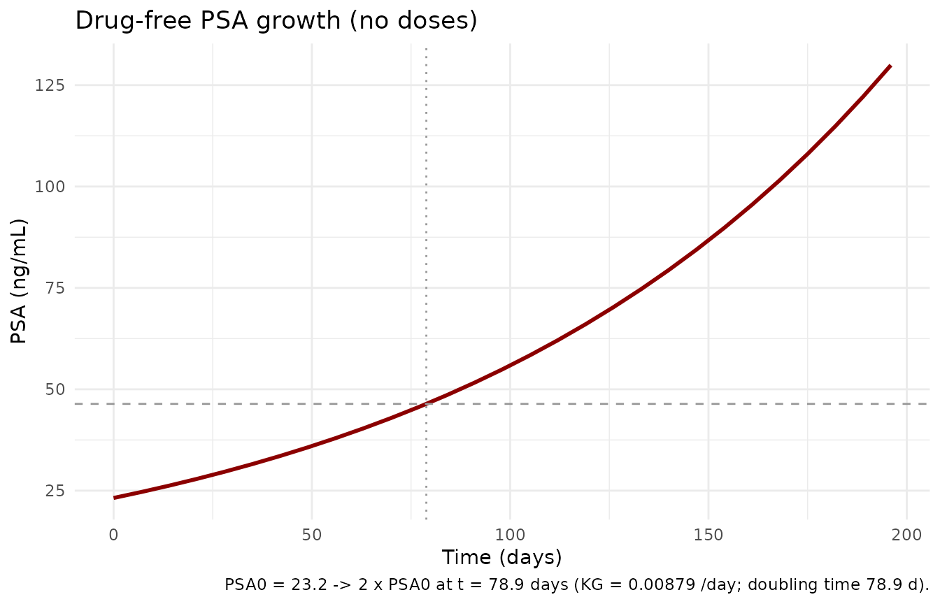
2. K-PD compartment decay
KP = 6000 /day is large by design (paper Results: “We
selected a large value of 6,000 to allow for a nearly instantaneous
dosing event”). The depot_kpd half-life is
log(2) / 6000 ~= 0.000116 day = 10 seconds. The vignette
plots depot_kpd(t) for a single AUC = 200 bolus over a
0.001-day (~ 1.5 minute) window so the rapid decay is visible.
events_pulse <- tibble(
  id = 1L,
  time = c(0, 1e-6, seq(1e-5, 0.001, length.out = 50)),
  evid = c(1L, rep(0L, 51L)),
  amt  = c(200, rep(0, 51L)),
  cmt  = c("depot_kpd", rep(NA_character_, 51L)),
  PRIOR_TAXANE = 0L, PRIOR_TAXANE_DAYS = 0
) |>
  arrange(time, desc(evid))

sim_pulse <- rxode2::rxSolve(mod_typ, events = events_pulse) |> as.data.frame()
#> ℹ omega/sigma items treated as zero: 'etalpsa0', 'etalkg', 'etalkres', 'etalkd0'

ggplot(sim_pulse |> filter(time > 0), aes(time * 86400, depot_kpd)) +  # x-axis in seconds
  geom_line(linewidth = 1, colour = "purple4") +
  labs(x = "Time after dose (seconds)", y = "depot_kpd (ng*h/mL; K-PD effect state)",
       title = "K-PD depot_kpd compartment decay after a single AUC = 200 bolus",
       caption = "Half-life log(2) / KP = log(2) / 6000 days ~= 10 seconds; depot_kpd is essentially impulsive on the day scale.") +
  theme_minimal()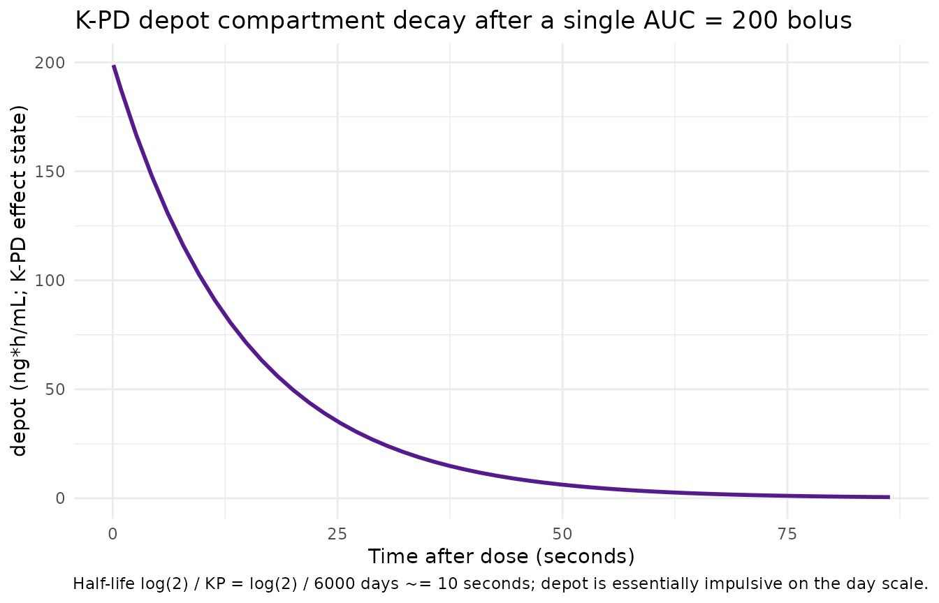
3. Resistance term decay
The exp(-k_res * t) factor that multiplies the
drug-inhibition term decays from 1 at study start with rate
k_res = 0.0113 /day (half-life log(2) / k_res ~= 61 days).
After ~180 days the drug-inhibition contribution is reduced to ~13
percent of its initial efficacy even at the same per-dose AUC –
consistent with the paper’s interpretation that “the developed DP model
for PSA was merely developed to provide acceptable individual PSA
predictions” and explicitly carries a resistance-development
mechanism.
resist_df <- tibble(
  time = seq(0, 200, by = 1),
  resistance = exp(-0.0113 * time)
)

half_life_kres <- log(2) / 0.0113

ggplot(resist_df, aes(time, resistance)) +
  geom_line(linewidth = 1, colour = "tomato3") +
  geom_hline(yintercept = 0.5, linetype = "dashed", colour = "grey60") +
  geom_vline(xintercept = half_life_kres, linetype = "dotted", colour = "grey60") +
  labs(x = "Time since treatment start (days)", y = "exp(-k_res * t) (unitless)",
       title = "Resistance multiplier on the drug-inhibition term",
       caption = sprintf("k_res = 0.0113 /day; half-life log(2)/k_res = %.1f days.", half_life_kres)) +
  theme_minimal()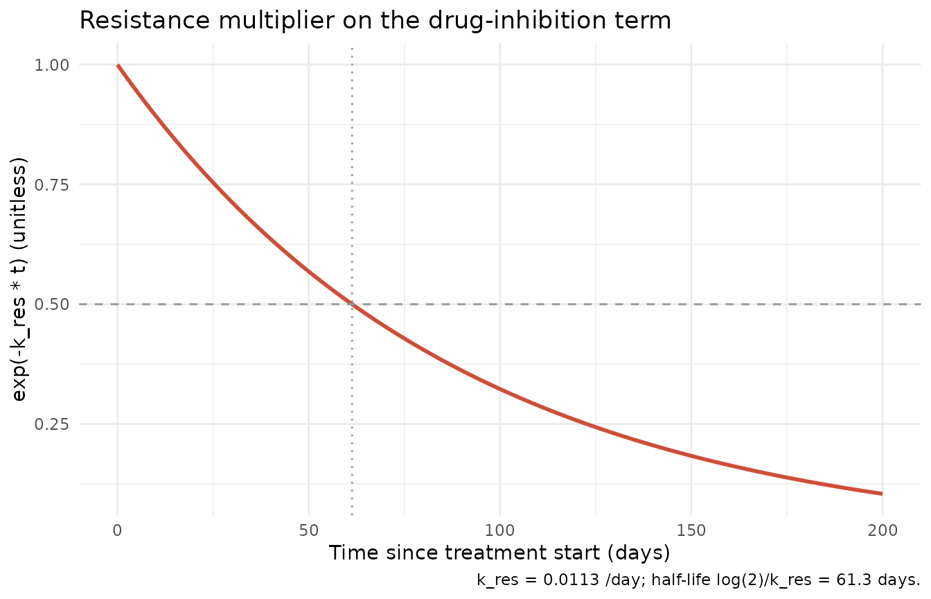
4. Dimensional analysis of the ODE system
| Term | Units | Reduces to |
|---|---|---|
kel * depot_kpd |
(1/day) * (ng*h/mL) |
(ng*h/mL)/day |
kg * PSA |
(1/day) * (ng/mL) |
(ng/mL)/day |
kd0 * exp(-k_res*t) * depot_kpd * PSA |
(L/(ng*h*day)) * 1 * (ng*h/mL) * (ng/mL) |
(ng/mL)/day |
The depot_kpd ODE reduces to (ng*h/mL)/day, consistent
with depot_kpd having units ng*h/mL (the AUC
area of one dose). The PSA ODE reduces to (ng/mL)/day,
consistent with PSA having units ng/mL. The
paper’s published unit string for KD0 (“ng*h/L /day /day”) is
dimensionally equivalent to L/(ng*h*day) once the product
KD0 * D is constrained to 1/day (the
inhibition-rate dimension that the PSA growth term KG has)
– 1 ug/L equals 1 ng/mL, so
(ng*h/mL)^-1 = (ug*h/L)^-1 = L/(ug*h). The numerical value
0.241 is unchanged.
Assumptions and deviations
Survival sub-model is not included. The paper’s parametric Weibull survival model (Table 3) is fit in R survreg on individual-predicted summaries from the DP model (time to PSA nadir, baseline PSA, PSA growth rate, ECOG score). It is a covariate regression on DP-model outputs rather than an ODE structure and so falls outside the scope of a
nlmixr2/rxode2model. Users who want the full DP-CO framework should run this model to predict PSA trajectories, derive the per-subject Tnadir / PSA0 / KG / ECOG-score summaries, then fit / apply the Weibull regression on those summaries downstream.Upstream eribulin popPK model is not encoded. The paper uses an external 3-compartment linear-elimination popPK model (Majid 2014 / van Hasselt 2013) with albumin, alkaline phosphatase, and total bilirubin on clearance to predict per-dose AUC values; those predictions then enter the DP model as the K-PD bolus amount. The two upstream popPK references are not on disk, and the DP model itself does not fix any PK parameter from those publications – it only consumes AUC as a dose input. Users with their own eribulin popPK model (or with per-patient AUC measurements) should supply AUC values via the
amtcolumn on each dose event; the vignette uses a single literature-typical placeholder of 200 ng*h/mL per dose.K-PD
depot_kpdcompartment naming. The paper’s “drug effect compartment D” is a K-PD construct that receives the per-dose predicted AUC as a bolus and decays atKP = 6000 /day. The compartment is nameddepot_kpdper the canonical K-PD register ininst/references/compartment-names.md; standard rxode2 dosing routing applies (amton anevid = 1row withcmt = "depot_kpd"deposits AUC into the K-PD state).Observation variable named
PSArather thanCc.Ccis canonical for drug concentrations in plasma; here the observation is endogenous serum PSA, not a drug concentration. Following the pattern used bytumorSizeinOuerdani_2015_pazopanib.Randphenylalanine_charbonneau_2021.R’s mechanistic-species naming, the observation variable isPSA(paper-native) with bare-suffixpropSdfor the proportional residual error.checkModelConventions()flags the non-Ccoutput as a warning; the deviation is intentional.LTBS proportional residual error mapping. The paper’s Methods (Structural model) states the PSA observations were log-transformed prior to fitting and analysed log-transform-both-sides (LTBS). The Table 2 residual-error CV% of 34.2 percent is mapped here to a linear-space proportional error
PSA ~ prop(0.342). For CV% in this range the linear-space proportional form and the strict log-normallnorm()form differ by less than 5 percent at the percentile tails; theprop()mapping matches the convention used by other LTBS models innlmixr2lib(e.g.,Buil-Bruna_2015_lanreotide.R).Per-dose AUC placeholder. For demonstration the vignette uses a single representative per-dose AUC of 200 ng*h/mL across all subjects and all cycles. Real per-subject AUC would vary with body size, hepatic function (albumin, ALP, bilirubin), and dose adjustments per the trial protocol. Supporting Table S1 of van Hasselt 2015 is referenced in the paper as the source of cohort-level AUC summaries but is not on disk for this extraction.
Population demographics gaps. The age range, weight range, race / ethnicity distribution, and dose range used for the cohort summary in
populationare not fully reported in the main paper text on disk. The paper’s Supporting Table S1 was not accompanying the PDF in the ingestion bundle; users with the supplement should consult it for the per-stratum demographic detail.PKNCA validation is omitted. This is a PSA disease-progression model with no drug-concentration ODE – there is no plasma drug concentration to run NCA on. The vignette substitutes the mechanistic-sanity checks above (drug-free pure growth = exp(KG*t), K-PD depot_kpd decay, resistance-term decay, dimensional analysis), matching the validation pattern used by
Ouerdani_2015_pazopanib.R(also a TGI / DP model).