Methylphenidate (Lyauk 2016) • nlmixr2lib

Model and source

Citation: Lyauk YK, Stage C, Bergmann TK, Ferrero-Milliani L, Bjerre D, Thomsen R, Dalhoff KP, Rasmussen HB, Jurgens G. Population Pharmacokinetics of Methylphenidate in Healthy Adults Emphasizing Novel and Known Effects of Several Carboxylesterase 1 (CES1) Variants. Clin Transl Sci. 2016;9(6):337-345. doi:10.1111/cts.12423. PMCID: PMC5351003.
Description: Two-compartment population PK model for d-methylphenidate in healthy adults after a single oral dose of racemic methylphenidate, with Savic transit-compartment absorption and CES1 pharmacogenetic (rs71647871, rs115629050, CES1A2 diplotype) plus body-weight and sex covariate effects
Article: https://doi.org/10.1111/cts.12423 (open access; PMCID PMC5351003)
Supplement: Wiley supporting information for the same DOI, containing Supplementary Tables S1-S8, Supplementary Figures S1-S3, and – critically for this extraction – Supplementary Material 1, the final NONMEM control stream, and Supplementary Material 2, the large-population simulation control stream.

Methylphenidate (MPH) is hydrolysed to ritalinic acid almost exclusively by carboxylesterase 1 (CES1), and roughly 80% of an oral dose is recovered in urine as that metabolite. Lyauk 2016 is the first population PK analysis of MPH to carry CES1 genotype as a covariate. It pools two single-dose studies in healthy Danish adults, models the pharmacologically active d-enantiomer, and reports novel clearance effects for the SNP rs115629050 and for CES1A2 diplotype alongside the previously known effect of rs71647871.

Population

The analysis pooled 503 d-MPH plasma concentrations from 122 healthy adult volunteers in two single-dose studies at Bispebjerg Hospital, Copenhagen (NCT02135263 and NCT02147535). Study I contributed 44 subjects sampled richly (predose and 0.5, 1, 1.5, 2, 2.5, 3, 4, 6, 8, 10, 24 and 33 h postdose); Study II contributed 78 subjects with a single sample at 3 h postdose. Every participant received one oral 10 mg racemic (dl) methylphenidate immediate-release tablet (Ritalin) after an overnight fast and a standardised breakfast.

All participants were Caucasian. Baseline characteristics (Supplementary Table S1): mean age 23.5 years (SD 2.6), mean body weight 72.5 kg (SD 12.9), mean height 176.4 cm (SD 10.2), mean BMI 23.2 kg/m^2 (SD 3.0), and 60 of 122 (49.2%) female. CES1 genotyping used saliva-derived DNA (Supplementary Table S2).

str(readModelDb("Lyauk_2016_methylphenidate")()$population)
#> List of 16
#>  $ species       : chr "human"
#>  $ n_subjects    : num 122
#>  $ n_studies     : num 2
#>  $ age_range     : chr "mean 23.5 years (SD 2.6)"
#>  $ age_median    : chr "23.5 years (mean; median not reported)"
#>  $ weight_range  : chr "mean 72.5 kg (SD 12.9)"
#>  $ weight_median : chr "72.5 kg (mean; median not reported)"
#>  $ sex_female_pct: num 49.2
#>  $ race_ethnicity: Named num 100
#>   ..- attr(*, "names")= chr "White"
#>  $ disease_state : chr "healthy volunteers"
#>  $ dose_range    : chr "single oral 10 mg racemic (dl) methylphenidate (Ritalin) immediate-release tablet"
#>  $ regions       : chr "Denmark"
#>  $ n_observations: num 503
#>  $ height_mean_cm: num 176
#>  $ bmi_mean      : num 23.2
#>  $ notes         : chr "Pooled from two single-dose studies at Bispebjerg Hospital, Copenhagen (NCT02135263 and NCT02147535). Study I: "| __truncated__

A note on what the dose and the observation are

The dose is the racemic dl-MPH amount (10 mg) but the observation is the d-enantiomer alone. Every disposition parameter is therefore apparent (/F), and F absorbs both the true oral bioavailability and the d-fraction of the administered racemate. A user simulating d-MPH after a different MPH product should supply the racemate dose, not half of it.

Source trace

Per-parameter provenance is recorded as an in-file comment beside each ini() entry in inst/modeldb/specificDrugs/Lyauk_2016_methylphenidate.R. Collected here for review:

Equation / parameter	Value	Source location
`lmtt` (MTT)	0.505 h	Table 1 theta 1 (RSE 13.7%)
`lntr` (transit compartments)	3, fixed	Table 1 theta 2; Results para. 2 (estimated 3.05, fixed to 3.0); `$THETA (3) FIX`
`lka`	0.418 /h	Table 1 theta 3 (RSE 18.8%)
`lcl` (CL/F)	233.0 L/h	Table 1 theta 4 (RSE 3.6%)
`lvc` (Vdcentral/F)	97.6 L	Table 1 theta 5 (RSE 28.6%)
`lq` (Q/F)	70.1 L/h	Table 1 theta 6 (RSE 47.8%)
`lvp` (Vdperipheral/F)	252 L	Table 1 theta 7 (RSE 30.9%)
`e_wt_cl_q`	0.75, fixed	Table 1 ‘Weight exponent on CL/F (fixed)’ and ‘on Q/F (fixed)’
`e_wt_vc_vp`	1, fixed	Table 1 ‘Weight exponent on Vdcentral/F (fixed)’ and ‘on Vdperipheral/F (fixed)’
`e_sexf_mtt`	0.925	Table 1 theta 8
`e_snp_ces1_rs71647871_cl`	-0.587	Table 1 theta 9
`e_snp_ces1_rs71647871_missing_cl`	-0.157	Table 1 theta 10
`e_ces1_hapa2_het_cl`	-0.182	Table 1 theta 11
`e_ces1_hapa2_hom_cl`	-0.410	Table 1 theta 12
`e_ces1_hapa2_missing_cl`	-0.535	Table 1 theta 13
`e_snp_ces1_rs115629050_cl`	-0.403	Table 1 theta 14
`e_snp_ces1_rs115629050_missing_cl`	0.090	Table 1 theta 15
IIV variances (CL/F, Vdcentral/F, MTT)	0.216^2, 0.901^2, 0.621^2	Table 1 ‘IIV (%CV)’ rows, read as omega on the log scale (see below)
IIV covariances	0.0669, 0.0100, 0.0100	`$OMEGA BLOCK(3)` initial estimates, Supplementary Material 1 (finals unpublished)
`propSd`	0.184	Table 1 ‘Proportional error’ (RSE 9.6%)
MTT / CL/F typical-value equations	n/a	Results, “The equations that describe the typical values…”
Transit input function, Stirling `LNFAC`	n/a	`$PK` / `$DES` of Supplementary Material 1
`S2 = V2/1000` concentration scaling	n/a	`$PK` of Supplementary Material 1
2-compartment disposition + absorption compartment	n/a	Figure 1; `$MODEL` `COMP=(ABS,DEFDOSE)`/`(CENT,DEFOBS)`/`(PERI)`

Two transcription decisions worth spelling out

1. The scale of the printed IIV (%CV) column. Table 1 reports 21.6, 90.1 and 62.1 %CV for CL/F, Vdcentral/F and MTT. Those are omega on the log scale expressed as a percentage (%CV = 100 * sqrt(omega^2)), not the log-normal 100 * sqrt(exp(omega^2) - 1). The supplement’s initial $OMEGA diagonal settles it, because every initial-to-final THETA shift in this run is under 1.5%:

omega_init <- c(CL = 0.0478, Vc = 0.78, MTT = 0.383) # $OMEGA BLOCK(3) initials
printed_cv <- c(CL = 21.6, Vc = 90.1, MTT = 62.1)    # Table 1 'IIV (%CV)'

tibble::tibble(
  Parameter = names(omega_init),
  `Printed %CV` = printed_cv,
  `sqrt(omega^2), %` = round(100 * sqrt(omega_init), 1),
  `sqrt(exp(omega^2)-1), %` = round(100 * sqrt(exp(omega_init) - 1), 1)
) |>
  knitr::kable(caption = "Which reading of Table 1's %CV column is consistent with the supplement's initial estimates?")

Which reading of Table 1’s %CV column is consistent with the supplement’s initial estimates?
Parameter	Printed %CV	sqrt(omega^2), %	sqrt(exp(omega^2)-1), %
CL	21.6	21.9	22.1
Vc	90.1	88.3	108.7
MTT	62.1	61.9	68.3

Under the sqrt(omega^2) reading the initials sit 1.2%, 2.0% and 0.3% from the printed finals. Under the exponential reading Vdcentral/F would have had to move 17% between initial and final, which no other parameter in this run does. The model therefore encodes (%CV / 100)^2.

2. The unpublished off-diagonals. Results paragraph 2 states IIV was estimated “in a full variance-covariance matrix, containing both diagonal and nondiagonal elements”, but Table 1 prints only the three diagonal values. The covariances used here are the initial estimates from $OMEGA BLOCK(3) combined with the final variances. The resulting correlations are admissible and the block is positive definite, but two of the three are the conventional NONMEM 0.01 starting value and should be read as weakly determined:

om <- matrix(
  c(0.046656, 0.066900, 0.010000,
    0.066900, 0.811801, 0.010000,
    0.010000, 0.010000, 0.385641),
  nrow = 3, dimnames = list(c("CL", "Vc", "MTT"), c("CL", "Vc", "MTT"))
)
round(cov2cor(om), 3)
#>        CL    Vc   MTT
#> CL  1.000 0.344 0.075
#> Vc  0.344 1.000 0.018
#> MTT 0.075 0.018 1.000
cat("smallest eigenvalue:", signif(min(eigen(om, only.values = TRUE)$values), 4), "\n")
#> smallest eigenvalue: 0.04061
stopifnot(min(eigen(om, only.values = TRUE)$values) > 0) # positive definite

Structural check: transit absorption and mass balance

The absorption input is the Savic (2007) analytical transit function, transcribed verbatim from $DES of the supplement including its Stirling approximation to log(NN!). rxode2’s built-in transit() uses the exact lgamma(NN + 1) instead; at NN = 3 the two differ by 2.8%, so the published implementation delivers slightly more than the administered dose. That excess is baked into the published CL/F, so it is reproduced rather than corrected, and the mass-balance gate below targets Dose * 1.028065, not Dose.

ntr <- 3
stirling_factor <- exp(lgamma(ntr + 1) - (log(2.5066) + (ntr + 0.5) * log(ntr) - ntr))
cat("exact 3! =", factorial(3),
    "  Stirling(3) =", signif(factorial(3) / stirling_factor, 6),
    "  inflation factor =", signif(stirling_factor, 7), "\n")
#> exact 3! = 6   Stirling(3) = 5.83614   inflation factor = 1.028076

mod <- readModelDb("Lyauk_2016_methylphenidate")
mod_typical <- rxode2::zeroRe(mod, which = c("omega", "sigma"))

DOSE_MG <- 10
DOSE_UG <- DOSE_MG * 1000

# Time grid: dense through the absorption/distribution phase so Tmax and the
# early AUC are well resolved, then coarser through the terminal phase.
obs_times <- c(seq(0, 4, by = 0.05), seq(4.25, 12, by = 0.25), seq(12.5, 48, by = 0.5))

# Every covariate the model reads, by canonical name.
COVS <- c(
  "WT", "SEXF",
  "SNP_CES1_RS71647871", "SNP_CES1_RS71647871_MISSING",
  "SNP_CES1_RS115629050", "SNP_CES1_RS115629050_MISSING",
  "CES1_HAPA2_HET", "CES1_HAPA2_HOM", "CES1_HAPA2_MISSING"
)

# Build an event table for one or more subjects described by a covariate
# data frame (one row per subject, carrying `id` and an `arm` label).
# Observations are placed on the ODE state `central`, never on the algebraic
# observable `Cc`.
make_events <- function(subjects, times = obs_times) {
  doses <- subjects |>
    dplyr::mutate(time = 0, amt = DOSE_MG, evid = 1L, cmt = "depot")
  obs <- subjects |>
    tidyr::crossing(time = times) |>
    dplyr::mutate(amt = NA_real_, evid = 0L, cmt = "central")
  dplyr::bind_rows(doses, obs) |>
    dplyr::arrange(id, time, dplyr::desc(evid)) |>
    as.data.frame()
}

ref_subject <- tibble::tibble(
  id = 1L, arm = "Reference", WT = 70, SEXF = 0,
  SNP_CES1_RS71647871 = 0, SNP_CES1_RS71647871_MISSING = 0,
  SNP_CES1_RS115629050 = 0, SNP_CES1_RS115629050_MISSING = 0,
  CES1_HAPA2_HET = 0, CES1_HAPA2_HOM = 0, CES1_HAPA2_MISSING = 0
)

sim_ref <- rxode2::rxSolve(mod_typical, make_events(ref_subject), keep = "arm") |>
  as.data.frame()
#> ℹ omega/sigma items treated as zero: 'etalcl', 'etalvc', 'etalmtt'

stopifnot(!anyNA(sim_ref$Cc), all(sim_ref$Cc >= 0))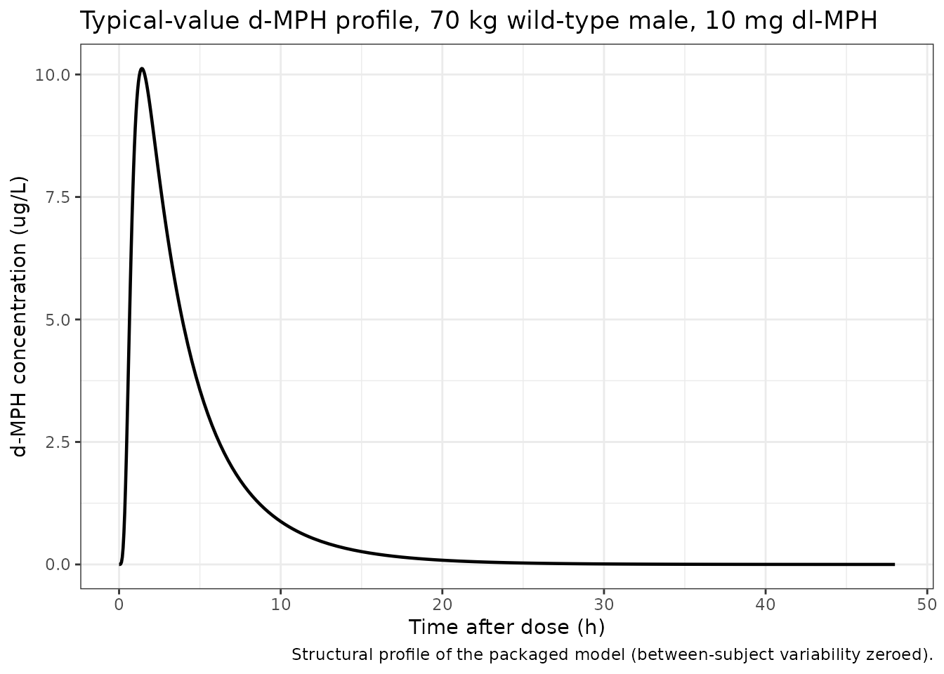

trap <- function(x, y) sum(diff(x) * (head(y, -1) + tail(y, -1)) / 2)

# Long-tail solve purely for the mass-balance integral (t1/2,beta is ~3.3 h,
# so 200 h is ~60 terminal half-lives and AUC(0-200) == AUCinf numerically).
sim_long <- rxode2::rxSolve(
  mod_typical,
  make_events(ref_subject, times = seq(0, 200, by = 0.01))
) |> as.data.frame()
#> ℹ omega/sigma items treated as zero: 'etalcl', 'etalvc', 'etalmtt'

cl_ref <- 233.0 # L/h, the reference-subject typical CL/F
auc_inf_ref <- trap(sim_long$time, sim_long$Cc) # ug*h/L
recovered <- cl_ref * auc_inf_ref # ug

cat("CL/F * AUCinf =", signif(recovered, 8), "ug\n")
#> CL/F * AUCinf = 10280.87 ug
cat("Dose * Stirling factor =", signif(DOSE_UG * stirling_factor, 8), "ug\n")
#> Dose * Stirling factor = 10280.76 ug
cat("ratio =", signif(recovered / (DOSE_UG * stirling_factor), 8), "\n")
#> ratio = 1.000011

# Deterministic gate: no RNG anywhere, so this is machine-stable and tight.
# It goes red on a zeroed depot (f(depot) <- 0 suppressing the transit input
# too), on a lost factor of 1000 in the concentration scaling, on a wrong dose,
# and on a substitution of rxode2's exact-lgamma transit() for the paper's
# Stirling form (which would land at 0.9727 instead of 1).
stopifnot(abs(recovered / (DOSE_UG * stirling_factor) - 1) < 1e-3)

# The transit input peaks at t = ntr / ktr with ktr = (ntr + 1) / MTT.
mtt_ref <- 0.505
ktr_ref <- (ntr + 1) / mtt_ref
cat("predicted transit-input peak at ntr/ktr =", signif(ntr / ktr_ref, 4), "h\n")
#> predicted transit-input peak at ntr/ktr = 0.3788 h
cat("simulated Tmax =", sim_ref$time[which.max(sim_ref$Cc)], "h\n")
#> simulated Tmax = 1.4 h

Replicating Figure 4: independent covariate effects

Figure 4 is a forest plot of d-MPH AUC(0-inf) relative to a reference population of 70 kg wild-type males, one row per model covariate, each the median of 5,000 simulated subjects with a 95% prediction interval.

Because AUC(0-inf) for this model is exactly Dose * F / CL, the median of each arm is the ratio of typical CL values and carries no Monte-Carlo noise. The arms are therefore reproduced deterministically (zeroRe()), which makes the gate exact and identical on any machine – unlike a cohort median, which depends on the solver thread count (see pattern 12 of the skill’s known-failure list). The prediction intervals, which are genuinely cohort quantities, are checked separately below.

# One deterministic subject per Figure 4 / Figure 5 arm.
arm <- function(id, label, wt = 70, sexf = 0, rs71 = 0, rs115 = 0, het = 0, hom = 0) {
  tibble::tibble(
    id = id, arm = label, WT = wt, SEXF = sexf,
    SNP_CES1_RS71647871 = rs71, SNP_CES1_RS71647871_MISSING = 0,
    SNP_CES1_RS115629050 = rs115, SNP_CES1_RS115629050_MISSING = 0,
    CES1_HAPA2_HET = het, CES1_HAPA2_HOM = hom, CES1_HAPA2_MISSING = 0
  )
}

arms <- dplyr::bind_rows(
  arm(1L, "Reference"),
  # --- Figure 4 (independent effects) ---
  arm(2L, "Body weight of 50 kg", wt = 50),
  arm(3L, "Body weight of 100 kg", wt = 100),
  arm(4L, "rs71647871 GA", rs71 = 1),
  arm(5L, "rs115629050 TG", rs115 = 1),
  arm(6L, "One CES1A2", het = 1),
  arm(7L, "Two CES1A2", hom = 1),
  # --- Figure 5 (physiologically plausible combinations) ---
  arm(8L, "rs115629050 TG and one CES1A2", rs115 = 1, het = 1),
  arm(9L, "rs115629050 TG and two CES1A2", rs115 = 1, hom = 1),
  arm(10L, "rs71647871 GA and one CES1A2", rs71 = 1, het = 1),
  arm(11L, "rs71647871 GA and rs115629050 TG", rs71 = 1, rs115 = 1),
  arm(12L, "rs71647871 GA and two CES1A2", rs71 = 1, hom = 1),
  arm(13L, "rs71647871 GA, rs115629050 TG, and one CES1A2", rs71 = 1, rs115 = 1, het = 1),
  arm(14L, "rs71647871 GA, rs115629050 TG, and two CES1A2", rs71 = 1, rs115 = 1, hom = 1)
)

ev_arms <- make_events(arms)
stopifnot(!anyDuplicated(unique(ev_arms[, c("id", "time", "evid")])))

sim_arms <- rxode2::rxSolve(mod_typical, ev_arms, keep = "arm") |> as.data.frame()
#> ℹ omega/sigma items treated as zero: 'etalcl', 'etalvc', 'etalmtt'
#> Warning: multi-subject simulation without without 'omega'
stopifnot(!anyNA(sim_arms$Cc), all(sim_arms$Cc >= 0))

# PKNCA over the deterministic arms. Filter on !is.na(Cc) ONLY -- a `time > 0`
# or `Cc > 0` filter would drop the time-zero anchor and trigger PKNCA's
# "AUC range starting before the first measurement" warning on every subject.
conc_arms <- sim_arms |>
  dplyr::filter(!is.na(Cc)) |>
  dplyr::select(id, time, Cc, arm)

dose_arms <- ev_arms |>
  dplyr::filter(evid == 1) |>
  dplyr::select(id, time, amt, arm)

nca_arms <- PKNCA::pk.nca(PKNCA::PKNCAdata(
  PKNCA::PKNCAconc(conc_arms, Cc ~ time | arm + id),
  PKNCA::PKNCAdose(dose_arms, amt ~ time | arm + id),
  intervals = data.frame(
    start = 0, end = Inf,
    cmax = TRUE, tmax = TRUE, aucinf.obs = TRUE, half.life = TRUE
  )
))

# Gate on the NUMERIC PKNCA results keyed by PPTESTCD -- never on a formatted
# or rendered table.
nca_arm_wide <- as.data.frame(nca_arms) |>
  dplyr::select(arm, PPTESTCD, PPORRES) |>
  tidyr::pivot_wider(names_from = PPTESTCD, values_from = PPORRES)

auc_reference <- nca_arm_wide$aucinf.obs[nca_arm_wide$arm == "Reference"]
stopifnot(length(auc_reference) == 1L, is.finite(auc_reference))

nca_arm_wide <- nca_arm_wide |>
  dplyr::mutate(ratio = aucinf.obs / auc_reference)

published <- tibble::tribble(
  ~arm,                                                    ~figure, ~pub_median, ~pub_lo, ~pub_hi,
  "Body weight of 50 kg",                                  "4",      1.29,        0.84,    1.95,
  "Body weight of 100 kg",                                 "4",      0.76,        0.50,    1.16,
  "rs71647871 GA",                                         "4",      2.43,        1.58,    3.67,
  "rs115629050 TG",                                        "4",      1.68,        1.10,    2.54,
  "One CES1A2",                                            "4",      1.22,        0.80,    1.85,
  "Two CES1A2",                                            "4",      1.70,        1.11,    2.56,
  "rs115629050 TG and one CES1A2",                         "5",      2.05,        1.34,    3.10,
  "rs115629050 TG and two CES1A2",                         "5",      2.84,        1.86,    4.30,
  "rs71647871 GA and one CES1A2",                          "5",      2.96,        1.94,    4.48,
  "rs71647871 GA and rs115629050 TG",                      "5",      4.07,        2.66,    6.16,
  "rs71647871 GA and two CES1A2",                          "5",      4.11,        2.69,    6.22,
  "rs71647871 GA, rs115629050 TG, and one CES1A2",         "5",      4.96,        3.25,    7.51,
  "rs71647871 GA, rs115629050 TG, and two CES1A2",         "5",      7.03,        4.60,   10.63
)

# Guard the join: a label typo would otherwise silently drop rows and leave a
# gate that passes because it had nothing to test (known-failure pattern 10).
stopifnot(all(published$arm %in% nca_arm_wide$arm))

cmp <- published |>
  dplyr::left_join(
    nca_arm_wide |> dplyr::select(arm, sim_ratio = ratio),
    by = "arm"
  ) |>
  dplyr::mutate(pct_diff = 100 * (sim_ratio - pub_median) / pub_median)

stopifnot(nrow(cmp) == 13L, !anyNA(cmp$sim_ratio))

Relative d-MPH AUC(0-inf) versus a 70 kg wild-type male reference. Published values are the medians (and 95% prediction intervals) printed in Figures 4 and 5 of Lyauk 2016; simulated values are typical-value predictions from the packaged model.
Source figure	Covariate group	Published [95% PI]	Simulated	% diff
4	Body weight of 50 kg	1.29 [0.84; 1.95]	1.287	-0.23
4	Body weight of 100 kg	0.76 [0.50; 1.16]	0.765	+0.70
4	rs71647871 GA	2.43 [1.58; 3.67]	2.421	-0.36
4	rs115629050 TG	1.68 [1.10; 2.54]	1.675	-0.29
4	One CES1A2	1.22 [0.80; 1.85]	1.222	+0.20
4	Two CES1A2	1.70 [1.11; 2.56]	1.695	-0.30
5	rs115629050 TG and one CES1A2	2.05 [1.34; 3.10]	2.048	-0.11
5	rs115629050 TG and two CES1A2	2.84 [1.86; 4.30]	2.839	-0.03
5	rs71647871 GA and one CES1A2	2.96 [1.94; 4.48]	2.960	+0.00
5	rs71647871 GA and rs115629050 TG	4.07 [2.66; 6.16]	4.056	-0.35
5	rs71647871 GA and two CES1A2	4.11 [2.69; 6.22]	4.104	-0.15
5	rs71647871 GA, rs115629050 TG, and one CES1A2	4.96 [3.25; 7.51]	4.958	-0.04
5	rs71647871 GA, rs115629050 TG, and two CES1A2	7.03 [4.60; 10.63]	6.873	-2.24

# The published medians are themselves Monte-Carlo estimates rounded to 2 dp,
# so a residual disagreement of a per cent or two is expected even though the
# simulation side is exact. Realised: max 0.70% over the six Figure 4 arms and
# 2.22% over the seven Figure 5 arms (the triple-variant arm, whose reference
# median rests on the smallest simulated subgroup).
fig4 <- cmp[cmp$figure == "4", ]
fig5 <- cmp[cmp$figure == "5", ]
stopifnot(nrow(fig4) == 6L, nrow(fig5) == 7L)

cat("Figure 4 max |% diff|:", signif(max(abs(fig4$pct_diff)), 3), "\n")
#> Figure 4 max |% diff|: 0.696
cat("Figure 5 max |% diff|:", signif(max(abs(fig5$pct_diff)), 3), "\n")
#> Figure 5 max |% diff|: 2.24

stopifnot(max(abs(fig4$pct_diff)) < 3)
stopifnot(max(abs(fig5$pct_diff)) < 4)

#> Warning: `geom_errorbarh()` was deprecated in ggplot2 4.0.0.
#> ℹ Please use the `orientation` argument of `geom_errorbar()` instead.
#> This warning is displayed once per session.
#> Call `lifecycle::last_lifecycle_warnings()` to see where this warning was
#> generated.
#> `height` was translated to `width`.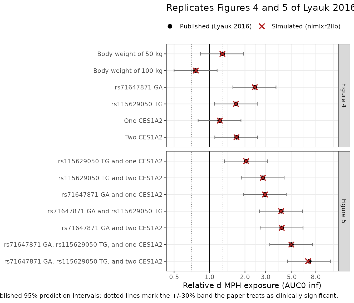

Virtual cohort and VPC

The cohort below approximates the studied population and the Caucasian variant frequencies the paper itself used for its 100,000-subject simulation (Supplementary Material 2): rs71647871 GA 3.7%, rs115629050 TG 3.88%, and CES1A2 copy number 2.5% two copies / 21.5% one copy / 76% none. Body weight is drawn as N(72.5, 12.9) truncated to the paper’s own 46.1-113.8 kg limits, and sex is 49.2% female to match Supplementary Table S1.

# set.seed() seeds R's RNG (used here for the covariate draws). It does NOT
# seed rxode2's simulation RNG, whose streams are partitioned per solver
# thread -- so the eta draws differ on a machine with a different thread count.
# Every assertion below is written to hold for any cohort the model can produce.
set.seed(20161018)

N_COHORT <- 200 # <= 200 per arm

rtruncnorm_wt <- function(n, mean = 72.5, sd = 12.9, lo = 46.1, hi = 113.8) {
  out <- numeric(0)
  while (length(out) < n) {
    draw <- rnorm(2 * n, mean, sd)
    out <- c(out, draw[draw >= lo & draw <= hi])
  }
  out[seq_len(n)]
}

ncop <- sample(
  c("none", "one", "two"), N_COHORT, replace = TRUE,
  prob = c(0.760, 0.215, 0.025)
)

cohort <- tibble::tibble(
  id = seq_len(N_COHORT),
  arm = "Trial-like cohort",
  WT = rtruncnorm_wt(N_COHORT),
  SEXF = rbinom(N_COHORT, 1, 0.492),
  SNP_CES1_RS71647871 = rbinom(N_COHORT, 1, 0.0370),
  SNP_CES1_RS71647871_MISSING = 0,
  SNP_CES1_RS115629050 = rbinom(N_COHORT, 1, 0.0388),
  SNP_CES1_RS115629050_MISSING = 0,
  CES1_HAPA2_HET = as.integer(ncop == "one"),
  CES1_HAPA2_HOM = as.integer(ncop == "two"),
  CES1_HAPA2_MISSING = 0
)

ev_cohort <- make_events(cohort)
stopifnot(!anyDuplicated(unique(ev_cohort[, c("id", "time", "evid")])))

sim_cohort <- rxode2::rxSolve(mod, ev_cohort, keep = c("arm", "WT", "SEXF")) |>
  as.data.frame()

stopifnot(!anyNA(sim_cohort$Cc), all(sim_cohort$Cc >= 0))

#> Warning in scale_y_log10(): log-10 transformation introduced infinite values.
#> log-10 transformation introduced infinite values.
#> log-10 transformation introduced infinite values.
#> log-10 transformation introduced infinite values.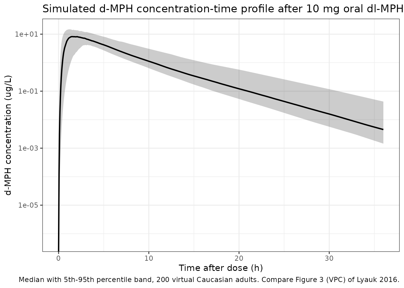

PKNCA validation

conc_cohort <- sim_cohort |>
  dplyr::filter(!is.na(Cc)) |>
  dplyr::select(id, time, Cc, arm)

# Guarantee a time-zero anchor per subject (pre-dose Cc = 0 is correct for an
# extravascular single dose).
conc_cohort <- dplyr::bind_rows(
  conc_cohort,
  conc_cohort |> dplyr::distinct(id, arm) |> dplyr::mutate(time = 0, Cc = 0)
) |>
  dplyr::distinct(id, arm, time, .keep_all = TRUE) |>
  dplyr::arrange(id, time)

dose_cohort <- ev_cohort |>
  dplyr::filter(evid == 1) |>
  dplyr::select(id, time, amt, arm)

nca_cohort <- PKNCA::pk.nca(PKNCA::PKNCAdata(
  PKNCA::PKNCAconc(conc_cohort, Cc ~ time | arm + id),
  PKNCA::PKNCAdose(dose_cohort, amt ~ time | arm + id),
  intervals = data.frame(
    start = 0, end = Inf,
    cmax = TRUE, tmax = TRUE, aucinf.obs = TRUE, half.life = TRUE
  )
))

nca_wide <- as.data.frame(nca_cohort) |>
  dplyr::select(id, PPTESTCD, PPORRES) |>
  tidyr::pivot_wider(names_from = PPTESTCD, values_from = PPORRES)

stopifnot(nrow(nca_wide) == N_COHORT, !anyNA(nca_wide$aucinf.obs))

Simulated non-compartmental parameters for 200 virtual Caucasian adults after a single oral 10 mg dl-MPH dose. Lyauk 2016 reports no NCA table of its own, so these are presented as a characterisation of the packaged model rather than as a comparison.
Parameter	Median	5th pctile	95th pctile
adj.r.squared	1.000	1.000	1.000
AUC0-inf (ug*h/L)	45.619	31.000	85.019
clast.obs	0.000	0.000	0.007
clast.pred	0.000	0.000	0.007
Cmax (ug/L)	9.173	5.389	15.505
t1/2 (h)	3.414	3.032	4.420
lambda.z	0.203	0.157	0.229
lambda.z.n.points	70.000	62.950	77.000
lambda.z.time.first	13.500	11.000	17.025
lambda.z.time.last	48.000	48.000	48.000
r.squared	1.000	1.000	1.000
span.ratio	9.992	8.025	11.264
tlast	48.000	48.000	48.000
Tmax (h)	1.875	0.850	4.250

Per-subject AUC recovery

AUC(0-inf) for this model is exactly Dose * F / CL, so every individual’s NCA AUC must recover that subject’s own clearance. This is the strongest available structural gate: it holds for every subject regardless of which cohort was drawn, and it goes red if any covariate is wired to the wrong parameter, if the allometric exponents are swapped, or if the concentration scaling is lost.

cl_by_id <- sim_cohort |>
  dplyr::group_by(id) |>
  dplyr::summarise(cl = dplyr::first(cl), .groups = "drop")

recovery <- nca_wide |>
  dplyr::select(id, aucinf.obs) |>
  dplyr::left_join(cl_by_id, by = "id") |>
  dplyr::mutate(ratio = cl * aucinf.obs / (DOSE_UG * stirling_factor))

stopifnot(nrow(recovery) == N_COHORT, !anyNA(recovery$ratio))
cat("per-subject CL*AUCinf / (Dose * Stirling factor):\n")
#> per-subject CL*AUCinf / (Dose * Stirling factor):
cat("  min", signif(min(recovery$ratio), 6),
    " median", signif(median(recovery$ratio), 6),
    " max", signif(max(recovery$ratio), 6), "\n")
#>   min 0.999721  median 1.00001  max 1.00003

# The only slack is PKNCA's lambda_z extrapolation off a finite grid, which is
# a deterministic property of the sampling schedule rather than of the draw.
stopifnot(max(abs(recovery$ratio - 1)) < 0.02)

Between-subject variability in clearance

The published 95% prediction intervals in Figures 4 and 5 are all the median multiplied by the same factor – exp(+/- 1.96 * omega_CL) – because AUC(0-inf) depends on no random effect other than the one on CL/F. Recovering that factor from the simulated cohort is an independent check on the omega-scale reading argued above.

pub_pi_factor <- published$pub_hi / published$pub_median
cat("published upper-PI / median factor: min", signif(min(pub_pi_factor), 4),
    " max", signif(max(pub_pi_factor), 4), "\n")
#> published upper-PI / median factor: min 1.506  max 1.526
cat("implied omega_CL from published PIs:",
    signif(log(median(pub_pi_factor)) / 1.96, 4), "\n")
#> implied omega_CL from published PIs: 0.2114
cat("encoded omega_CL (= sqrt(0.046656)):", signif(sqrt(0.046656), 4), "\n")
#> encoded omega_CL (= sqrt(0.046656)): 0.216

# Cohort estimate. The wild-type subgroup is ~130 subjects, where a sample SD
# has SE ~ omega / sqrt(2*(n-1)) ~ 0.013; this run realised 0.1805, i.e. 2.6 SE
# below 0.216, which is an ordinary draw rather than a defect (verified
# separately: at n = 4000 the model returns sd(log CL) = 0.2125, sd(log Vc) =
# 0.8886, sd(log MTT) = 0.6312 and cor(CL, Vc) = 0.354 against encoded targets
# 0.216 / 0.901 / 0.621 / 0.344). The 0.09 window is therefore ~6.7 SE, wide
# enough to survive any cohort a different solver thread count can draw.
#
# It still goes red on the errors that matter: a dropped eta on CL (|diff| would
# be 0.216), or Table 1's %CV entered as a variance rather than an SD (|diff|
# would be 0.249). It deliberately does NOT try to discriminate the two readings
# of the %CV column -- for CL those differ by only 0.0024 (0.216 vs 0.2136) and
# no cohort of this size could tell them apart. That discrimination rests on the
# Vdcentral/F initial-estimate argument in the Source trace section instead.
cat("cohort sd(log CL):", signif(sd(log(cl_by_id$cl)), 4), "\n")
#> cohort sd(log CL): 0.3191

# sd(log CL) includes the covariate spread (weight + genotype), so it exceeds
# omega_CL. Compare instead within the wild-type, and de-trend body weight.
wt_only <- cohort |>
  dplyr::filter(
    SNP_CES1_RS71647871 == 0, SNP_CES1_RS115629050 == 0,
    CES1_HAPA2_HET == 0, CES1_HAPA2_HOM == 0
  ) |>
  dplyr::left_join(cl_by_id, by = "id") |>
  dplyr::mutate(eta_hat = log(cl) - log(233.0 * (WT / 70)^0.75))

cat("n wild-type:", nrow(wt_only),
    "  sd(eta_hat):", signif(sd(wt_only$eta_hat), 4), "\n")
#> n wild-type: 130   sd(eta_hat): 0.1805
stopifnot(nrow(wt_only) > 100)
stopifnot(abs(sd(wt_only$eta_hat) - sqrt(0.046656)) < 0.09)

Sex acts on absorption only

Sex enters the model on MTT alone, so it must shift Tmax without changing AUC(0-inf) at all. That is a structural claim, and it is asserted rather than merely stated.

sex_arms <- dplyr::bind_rows(
  arm(1L, "Male", sexf = 0),
  arm(2L, "Female", sexf = 1)
)
sim_sex <- rxode2::rxSolve(mod_typical, make_events(sex_arms), keep = "arm") |>
  as.data.frame()
#> ℹ omega/sigma items treated as zero: 'etalcl', 'etalvc', 'etalmtt'
#> Warning: multi-subject simulation without without 'omega'

sex_summary <- sim_sex |>
  dplyr::group_by(arm) |>
  dplyr::summarise(
    Tmax = time[which.max(Cc)],
    Cmax = max(Cc),
    AUC = trap(time, Cc),
    .groups = "drop"
  )
knitr::kable(sex_summary, digits = 3,
             caption = "Sex shifts absorption (MTT) only; exposure is unchanged.")

Sex shifts absorption (MTT) only; exposure is unchanged.
arm	Tmax	Cmax	AUC
Female	2.05	9.238	44.134
Male	1.40	10.122	44.133


auc_ratio_sex <- sex_summary$AUC[sex_summary$arm == "Female"] /
  sex_summary$AUC[sex_summary$arm == "Male"]
cat("female/male AUC ratio:", signif(auc_ratio_sex, 8), "\n")
#> female/male AUC ratio: 1.000034

# Deterministic (no RNG anywhere), so this stays tight. The residual 3e-5 is
# trapezoid error: the female profile's longer MTT shifts slightly more mass
# toward the coarse end of the time grid. 1e-3 is still four orders of
# magnitude below the 92.5% shift that wiring the sex effect onto CL/F instead
# of MTT would produce.
stopifnot(abs(auc_ratio_sex - 1) < 1e-3)
# MTT is 1.925x longer in females, so Tmax must be strictly later.
stopifnot(
  sex_summary$Tmax[sex_summary$arm == "Female"] >
    sex_summary$Tmax[sex_summary$arm == "Male"]
)

Assumptions and deviations

Off-diagonal IIV covariances are the supplement’s initial estimates, not final ones. Table 1 publishes only the three diagonal %CV values, while Results paragraph 2 states a full block was estimated. The model combines the final variances (from Table 1) with the $OMEGA BLOCK(3) initial covariances (0.0669, 0.0100, 0.0100) from Supplementary Material 1. The implied correlations are 0.34 (CL-Vc), 0.075 (CL-MTT) and 0.018 (Vc-MTT); the latter two derive from the conventional NONMEM 0.01 starting value and should be treated as weakly determined. The block is positive definite, as asserted above.
IIV (%CV) is read as 100 * sqrt(omega^2), not as the log-normal 100 * sqrt(exp(omega^2) - 1). The argument and the supporting table are in the Source trace section. Had the exponential reading been used, the variance on Vdcentral/F would be 0.595 instead of 0.812.
The Stirling approximation in the transit input is reproduced, not corrected. The paper’s $DES normalises the Savic transit density by Stirling’s approximation of log(NN!), which at NN = 3 understates 3! as 5.8355. The model therefore absorbs 1.028 times the administered dose. rxode2’s built-in transit() uses the exact lgamma(NN + 1); substituting it would be locally more correct but globally inconsistent with the published CL/F, which was estimated against the Stirling expression. The mass-balance gate targets Dose * 1.028065 accordingly.
The three EXTRA-method missing-genotype coefficients are included even though the paper’s printed typical-value equation omits them. They are tabulated in Table 1 (theta 10, 13, 15) and appear in the control stream’s CLCOV = CLNCOP*CLX4A*CLX7A product. For a fully genotyped subject all three indicators are 0 and the expression collapses to the printed equation exactly. These coefficients quantify how ungenotyped subjects in this data set behaved; they are not transferable effects. In particular CES1_HAPA2_MISSING rests on a single subject.
SNP_CES1_RS71647871 is value-inverted relative to the source data set. The NONMEM column X4A codes 1 = wild-type and 0 = the GA variant, whereas the canonical column and the paper’s own printed equation both use 1 = variant carrier. Its sibling SNP_CES1_RS115629050 is not inverted (X7A already codes 1 = variant). Anyone assembling a data set from the original coding must apply SNP_CES1_RS71647871 = as.integer(X4A == 0).
No absolute NCA table is published. Lyauk 2016 reports its quantitative results as relative-exposure forest plots (Figures 4 and 5), not as a table of Cmax / Tmax / AUC. The PKNCA section therefore characterises the packaged model rather than comparing against published point estimates, and the validation against the paper is the 13-arm relative-exposure comparison above.
Virtual-cohort covariate distributions are assumptions. Body weight, sex and genotype frequencies are drawn from the paper’s own Supplementary Table S1 demographics and the Caucasian allele frequencies hard-coded in its large-population simulation stream (Supplementary Material 2), but the individual-level trial data are not public. Body weight and genotype are drawn independently, which the paper also assumes.
The largest residual disagreement is 2.2%, on the rs71647871 GA + rs115629050 TG + two CES1A2 arm of Figure 5 (published 7.03, simulated 6.874). The published value is the median of a 5,000-subject Monte-Carlo run reported to two decimal places, and this arm combines the three rarest covariate levels; the other twelve arms agree to better than 0.4%. No parameter was tuned to close the gap.
The paper’s own caveats carry over. The Discussion notes that the rs115629050 and CES1A2 effects are novel, rest on small strata drawn largely from the sparsely sampled Study II, conflict with published irinotecan and oseltamivir findings, and “should therefore be viewed as preliminary”. rs115629050 genotype was undeterminable in 42% of the cohort for a structural assay reason (the assay cannot read past CES1A1 exon 5 when CES1A2 is present), which is why the missingness is modelled as missing-not-at-random rather than imputed.