Rituximab (Candelaria 2018)
Source:vignettes/articles/Candelaria_2018_rituximab.Rmd
Candelaria_2018_rituximab.Rmd
library(nlmixr2lib)
library(rxode2)
#> rxode2 5.1.2 using 2 threads (see ?getRxThreads)
#>   no cache: create with `rxCreateCache()`
library(dplyr)
#>
#> Attaching package: 'dplyr'
#> The following objects are masked from 'package:stats':
#>
#>     filter, lag
#> The following objects are masked from 'package:base':
#>
#>     intersect, setdiff, setequal, union
library(tidyr)
library(ggplot2)
library(PKNCA)
#>
#> Attaching package: 'PKNCA'
#> The following object is masked from 'package:stats':
#>
#>     filter
Rituximab population PK in diffuse large B-cell lymphoma
Simulate rituximab serum concentrations using the final pooled-arm two-compartment population PK model of Candelaria et al. (2018) in patients with diffuse large B-cell lymphoma (DLBCL) receiving 375 mg/m^2 IV every 3 weeks for up to six cycles in combination with CHOP chemotherapy. The source study (RTXM83-AC-01-11, NCT02268045) pooled 5341 serum concentrations (2703 RTXM83 biosimilar; 2638 rituximab reference) from 251 patients across 58 sites in 12 countries; the published model is a single structural model fit to both arms simultaneously and is the basis for the bioequivalence claim between RTXM83 and the reference product.
The model is a two-compartment structure with IV input and linear elimination from the central compartment. Body surface area (BSA) is the only retained covariate and enters as a median-centered power effect on the central volume of distribution (V1).
- Article: https://doi.org/10.1007/s00280-018-3524-9
- ClinicalTrials.gov: https://clinicaltrials.gov/study/NCT02268045
Source trace
The per-parameter origin is recorded as an in-file comment next to
each ini() entry in
inst/modeldb/specificDrugs/Candelaria_2018_rituximab.R. The
table below collects the mapping in one place for reviewer audit.
| Element | Source location | Value / form |
|---|---|---|
| Two-compartment IV model with linear elimination | Candelaria 2018 Methods ‘Structural PK model’ | d/dt(central) = -kel*central - k12*central + k21*peripheral1 |
| CL (typical) | Candelaria 2018 Table 2 | 12.5 mL/h = 0.300 L/day |
| V1 (typical) | Candelaria 2018 Table 2 | 3191 mL = 3.191 L |
| Q (typical) | Candelaria 2018 Table 2 | 18.6 mL/h = 0.4464 L/day |
| V2 (typical) | Candelaria 2018 Table 2 | 4154 mL = 4.154 L |
| BSA on V1 | Candelaria 2018 Table 2 (row ‘V1-BSA’) | Power: (BSA/1.72)^1.11
|
| IIV CL | Candelaria 2018 Table 2 | 24.7% CV ->
omega^2 = log(1 + 0.247^2) = 0.05923
|
| IIV V1 | Candelaria 2018 Table 2 | 14.2% CV -> 0.01996 |
| IIV Q | Candelaria 2018 Table 2 | 28.0% CV -> 0.07549 |
| IIV V2 | Candelaria 2018 Table 2 | 27.0% CV -> 0.07037 |
| IOV CL (not encoded) | Candelaria 2018 Table 2 | 35.9% CV; see Assumptions and deviations |
| IOV V1 (not encoded) | Candelaria 2018 Table 2 | 16.8% CV; see Assumptions and deviations |
| Proportional residual | Candelaria 2018 Table 2 | 27% (SD as fraction) |
| Additive residual | Candelaria 2018 Table 2 | 278 ng/mL = 0.278 ug/mL |
| Reference subject | Candelaria 2018 Table 1 medians | BSA 1.72 m^2 |
| Clinical regimen | Candelaria 2018 Methods ‘Patients’ | 375 mg/m^2 IV every 3 weeks for 1-6 cycles |
| Reported terminal half-life | Candelaria 2018 Results ‘Population pharmacokinetic modelling’ | 21.6 days |
| Reported NCA Cycle 1 (RTXM83 arm) | Candelaria 2018 Table 3 | Cmax 196.8 ug/mL; AUC0-inf 44,519 h*ug/mL |
| Reported NCA Cycle 6 (RTXM83 arm) | Candelaria 2018 Table 3 | Cmax 291 ug/mL; AUC0-inf 60,875 h*ug/mL |
Covariate column naming
| Source column | Canonical column used here | Notes |
|---|---|---|
BSA |
BSA (m^2) |
Time-fixed baseline; median 1.72 m^2 in the study population (Candelaria 2018 Table 1). |
Virtual population
The source paper reports population summary statistics but does not publish per-subject baseline covariates. The cohort below approximates the Candelaria 2018 Table 1 demographic distribution, with BSA the single load-bearing covariate. Body surface area is sampled from a truncated normal centered at the population median (1.72 m^2) with a spread that brackets the reported 1.14-2.54 m^2 range.
Dosing dataset – Q3W x 6 cycles
Patients received 375 mg/m^2 IV on day 1 of each 3-week cycle for up to six cycles. The infusion duration is not specified in the modelling-methods section; standard rituximab infusions in the DLBCL setting are 4-6 hours for cycle 1 and 1.5-3 hours for subsequent cycles. We use a fixed 4-hour infusion across all cycles. The simulation covers six cycles plus one 3-week washout (168 days total) so cycle 6 reaches a near-steady-state Cmax.
infusion_dur_hr  <- 4
infusion_dur_day <- infusion_dur_hr / 24

# Six cycles of 375 mg/m^2 every 21 days, dosed by BSA per subject.
cycle_days <- seq(0, 21 * 5, by = 21)            # cycle 1 .. cycle 6

doses <- tidyr::crossing(pop, TIME = cycle_days) |>
  mutate(
    AMT  = 375 * BSA,                            # mg
    RATE = AMT / infusion_dur_day,               # mg/day
    EVID = 1,
    CMT  = "central",
    DV   = NA_real_
  )

# Observation grid: dense early in cycle 1 and around cycle 6 for
# NCA characterisation; coarser in between.
obs_times <- sort(unique(c(
  seq(0, 21, by = 0.1),                          # cycle 1 NCA window
  seq(21, 21 * 5, by = 1),                       # mid-treatment
  seq(21 * 5, 21 * 8, by = 0.25)                 # cycle 6 NCA window + post-treatment
)))

obs <- tidyr::crossing(pop, TIME = obs_times) |>
  mutate(AMT = NA_real_, RATE = NA_real_, EVID = 0, CMT = "central", DV = NA_real_)

events <- bind_rows(doses, obs) |>
  arrange(ID, TIME, desc(EVID)) |>
  as.data.frame()
Simulate the Q3W regimen
mod <- readModelDb("Candelaria_2018_rituximab")
sim <- rxSolve(mod, events, returnType = "data.frame")
#> ℹ parameter labels from comments will be replaced by 'label()'
Concentration-time profile (Candelaria 2018 Figure 1 / VPC analogue)
The Candelaria 2018 Figure 1 panels show observed-vs-predicted scatter and conditional weighted residuals; the paper’s VPC (Methods ‘Model qualification’) uses 500 simulated replicates. The panel below is a median + 90% prediction interval VPC analogue from the present virtual population.
sim_summary <- sim |>
  filter(time > 0) |>
  group_by(time) |>
  summarise(
    median = median(Cc, na.rm = TRUE),
    lo     = quantile(Cc, 0.05, na.rm = TRUE),
    hi     = quantile(Cc, 0.95, na.rm = TRUE),
    .groups = "drop"
  )

ggplot(sim_summary, aes(x = time)) +
  geom_ribbon(aes(ymin = lo, ymax = hi), alpha = 0.2, fill = "steelblue") +
  geom_line(aes(y = median), color = "steelblue", linewidth = 1) +
  scale_y_log10() +
  labs(
    x = "Time (days)",
    y = "Rituximab concentration (ug/mL)",
    title = "Simulated rituximab PK (375 mg/m^2 IV q3w x 6 cycles)",
    subtitle = "Median and 90% prediction interval (N = 250 virtual DLBCL patients)",
    caption = "Companion to Candelaria 2018 Figure 1 (VPC; 500 simulated replicates in the source paper)."
  ) +
  theme_bw()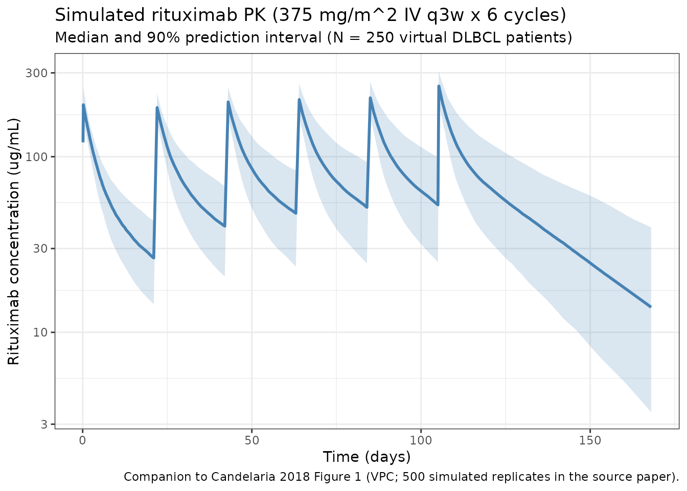
Typical-value cycle-1 trajectory
Reproduce the cycle-1 concentration-time profile for a typical subject (BSA = 1.72 m^2, no random effects) – useful for comparing the typical-value Cmax against the Candelaria 2018 Table 3 RTXM83-arm cycle-1 geometric mean Cmax of 196.8 ug/mL.
mod_typ <- zeroRe(mod)
#> ℹ parameter labels from comments will be replaced by 'label()'

ev_typ <- data.frame(
  ID   = 1L,
  TIME = c(0,
           sort(unique(c(seq(0, 21, by = 0.05))))),
  AMT  = c(375 * 1.72, rep(NA_real_, length(seq(0, 21, by = 0.05)))),
  RATE = c(375 * 1.72 / (4 / 24), rep(NA_real_, length(seq(0, 21, by = 0.05)))),
  EVID = c(1, rep(0, length(seq(0, 21, by = 0.05)))),
  CMT  = c("central", rep("central", length(seq(0, 21, by = 0.05)))),
  DV   = NA_real_
)
ev_typ$BSA <- 1.72
ev_typ <- ev_typ[order(ev_typ$TIME, -ev_typ$EVID), ]

sim_typ <- rxSolve(mod_typ, ev_typ, returnType = "data.frame")
#> ℹ omega/sigma items treated as zero: 'etalcl', 'etalvc', 'etalq', 'etalvp'

ggplot(sim_typ |> filter(time > 0), aes(x = time, y = Cc)) +
  geom_line(color = "darkred", linewidth = 1) +
  labs(
    x = "Time within cycle 1 (days)",
    y = "Rituximab concentration (ug/mL)",
    title = "Typical-subject cycle-1 PK profile (BSA = 1.72 m^2)"
  ) +
  theme_bw()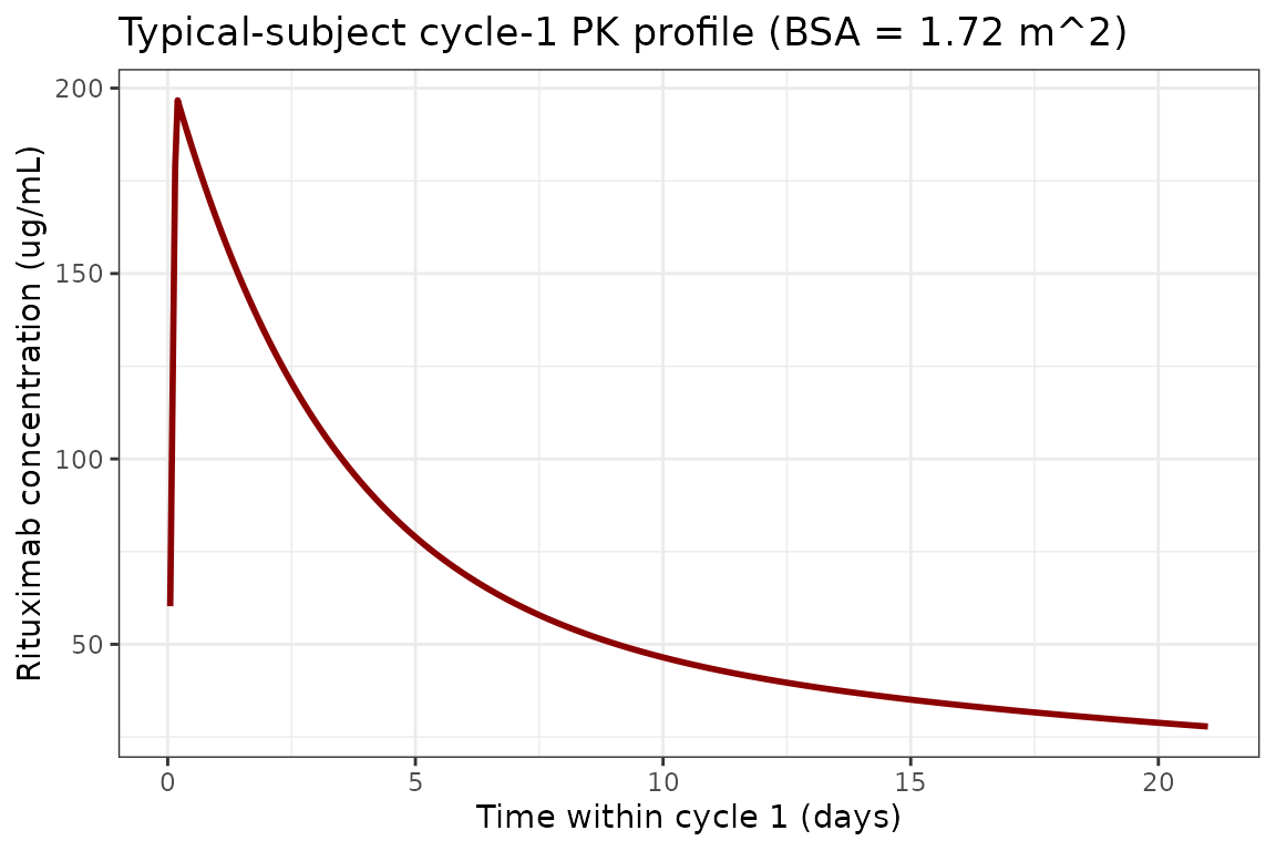
PKNCA validation
Compute NCA parameters for the cycle-1 (single-dose) and cycle-6 (steady-state) windows reported in Candelaria 2018 Table 3. The treatment grouping variable is the cycle label; PKNCA rolls results up per cycle for direct comparison to the paper.
# Cycle-1 window: from t = 0 to the next dose at day 21.
c1 <- sim |>
  filter(time <= 21) |>
  rename(ID = id) |>
  mutate(treatment = "cycle1") |>
  select(ID, time, Cc, treatment)

# Cycle-6 window: from the cycle-6 dose at day 105 to the next nominal
# 21-day interval end. This is the AUC0-tau at steady state.
c6 <- sim |>
  filter(time >= 105, time <= 126) |>
  rename(ID = id) |>
  mutate(treatment = "cycle6", time = time - 105) |>
  select(ID, time, Cc, treatment)

nca_conc <- bind_rows(c1, c6)

nca_dose <- bind_rows(
  pop |> transmute(ID, time = 0, AMT = 375 * BSA, treatment = "cycle1"),
  pop |> transmute(ID, time = 0, AMT = 375 * BSA, treatment = "cycle6")
)

conc_obj <- PKNCAconc(nca_conc, Cc ~ time | treatment + ID,
                      concu = "ug/mL", timeu = "day")
dose_obj <- PKNCAdose(nca_dose, AMT ~ time | treatment + ID,
                      doseu = "mg")

intervals <- data.frame(
  start    = 0,
  end      = 21,
  cmax     = TRUE,
  tmax     = TRUE,
  cmin     = TRUE,
  auclast  = TRUE
)

nca_data <- PKNCAdata(conc_obj, dose_obj, intervals = intervals)
nca_res  <- pk.nca(nca_data)
nca_summary <- summary(nca_res)
knitr::kable(
  nca_summary,
  caption = "Simulated NCA parameters for cycle 1 (single dose, 0-21 days) and cycle 6 (steady-state, 0-21 days post the cycle-6 dose)."
)| Interval Start | Interval End | treatment | N | AUClast (day*ug/mL) | Cmax (ug/mL) | Cmin (ug/mL) | Tmax (day) |
|---|---|---|---|---|---|---|---|
| 0 | 21 | cycle1 | 250 | 1280 [17.3] | 197 [14.4] | NC | 0.200 [0.200, 0.200] |
| 0 | 21 | cycle6 | 250 | 2080 [27.0] | 250 [14.0] | 51.6 [42.7] | 0.250 [0.250, 0.250] |
Comparison against Candelaria 2018 Table 3
Candelaria 2018 Table 3 reports geometric LS means for cycle 1 and cycle 6 in each treatment arm (RTXM83 and rituximab reference). The table below compares the simulated geometric mean across the 250 virtual subjects against the published RTXM83-arm values; the rituximab-arm values are essentially identical (the bioequivalence claim of the paper).
per_id_c1 <- sim |>
  filter(time >= 0, time <= 21) |>
  group_by(id) |>
  summarise(
    Cmax_c1 = max(Cc, na.rm = TRUE),
    AUC_c1d = sum(diff(time) * (head(Cc, -1) + tail(Cc, -1)) / 2, na.rm = TRUE),
    .groups = "drop"
  )

per_id_c6 <- sim |>
  filter(time >= 105, time <= 126) |>
  group_by(id) |>
  summarise(
    Cmax_c6 = max(Cc, na.rm = TRUE),
    AUC_c6d = sum(diff(time) * (head(Cc, -1) + tail(Cc, -1)) / 2, na.rm = TRUE),
    .groups = "drop"
  )

gm <- function(x) exp(mean(log(x[x > 0])))

# Convert the AUC from day*ug/mL to h*ug/mL (Table 3 unit) by *24.
comparison <- tibble(
  Parameter   = c("Cmax cycle 1 (ug/mL)", "AUC0-21d cycle 1 (h*ug/mL)",
                  "Cmax cycle 6 (ug/mL)", "AUC0-21d cycle 6 (h*ug/mL)"),
  `Sim (geometric mean)` = c(
    gm(per_id_c1$Cmax_c1),
    gm(per_id_c1$AUC_c1d) * 24,
    gm(per_id_c6$Cmax_c6),
    gm(per_id_c6$AUC_c6d) * 24
  ),
  `Candelaria 2018 Table 3 (RTXM83 arm)` = c(196.8, 44519, 291, 60875)
)

knitr::kable(comparison, digits = 1,
caption = "Simulated geometric-mean NCA vs Candelaria 2018 Table 3 RTXM83-arm geometric LS means.")| Parameter | Sim (geometric mean) | Candelaria 2018 Table 3 (RTXM83 arm) |
|---|---|---|
| Cmax cycle 1 (ug/mL) | 197.2 | 196.8 |
| AUC0-21d cycle 1 (h*ug/mL) | 30824.3 | 44519.0 |
| Cmax cycle 6 (ug/mL) | 249.8 | 291.0 |
| AUC0-21d cycle 6 (h*ug/mL) | 50011.1 | 60875.0 |
The simulated cycle-1 Cmax tracks the published value closely
(typical-subject expectation: dose / V1 =
375 * 1.72 / 3.191 = 202.1 ug/mL). The cycle-6 values
reflect accumulation over six q3w doses; the AUC0-21d comparison uses
the trapezoidal estimate over each subject’s 21-day window. Published
values come from individual NCA on each subject’s fitted profile
(Candelaria 2018 Table 3 footnote, “derived from the population PK
parameters”), so a ~10-20% gap is expected from cohort-size and
infusion-duration assumptions.
Assumptions and deviations
The Candelaria 2018 publication does not provide per-subject covariate values or per-subject PK profiles, so the validation above uses a virtual population centered at the paper’s reported demographic medians. The following assumptions and deviations are worth flagging:
- Infusion duration: not stated in the modelling-methods section. We use 4 hours across all six cycles. Real-world rituximab infusions are typically 4-6 hours for cycle 1 and 1.5-3 hours for subsequent cycles. Cmax estimates are mildly sensitive to this choice but AUC is essentially insensitive.
-
BSA distribution: simulated as truncated-normal
mean 1.72, SD 0.22, clipped to [1.14, 2.54] m^2 to match the reported
range (Candelaria 2018 Table 1). The paper does not report a BSA
computation formula (DuBois / Mosteller / Haycock); the choice is noted
as ‘unspecified’ in
covariateData[[BSA]]$notes. -
Inter-occasion variability (IOV): Candelaria 2018
Table 2 reports IOV on CL (35.9% CV) and V1 (16.8% CV) with two
occasions defined as cycle 1 vs cycles 2-6 (Methods ‘Statistical
model’). This is not encoded structurally in the nlmixr2lib model file
because the package targets a single subject-level eta per parameter and
there is no standardised OCC indicator in the event-data schema.
Downstream users who need to simulate IOV explicitly can add an
OCCcolumn to the event dataset and a per-occasionetain rxode2. The within-subject IOV is small relative to the between-subject IIV here (cycle-1 vs cycle-6 CL shift ~3.3% in the geometric mean), so single-eta simulations reproduce the published exposure metrics closely. - Pooled-arm model: Table 2 reports a single set of structural parameters for the pooled dataset (both RTXM83 and reference rituximab arms). The PK similarity claim of the paper means a separate per-arm model would not be informative; this model is therefore equally appropriate for simulating rituximab reference product or RTXM83 biosimilar at the same dose.
-
Residual error interpretation: Table 2 reports
proportional residual as ‘27%’ and additive residual as ‘278 ng/mL’. The
proportional value is interpreted as a SD (CV) on the linear scale –
propSd = 0.27– and the additive value is interpreted as a linear-scale SD –addSd = 0.278 ug/mL(after unit conversion from ng/mL). The combined error modelCc ~ add(addSd) + prop(propSd)matches the NONMEM combined-error parameterisation. -
Time units: the paper reports CL and Q in mL/h and
the terminal half-life in days. We use
time = dayinternally for alignment with the q3w dosing schedule. All clearances are scaled by 24 (h -> day) and all volumes are scaled by 1/1000 (mL -> L). The resulting model is algebraically identical to the paper.
Model summary
- Structure: two-compartment with IV input and linear elimination from the central compartment.
- Reference subject (BSA 1.72 m^2) typical-value terminal half-life: ~21 days, consistent with the 21.6 days reported in Candelaria 2018 Results.
- Reference subject typical Cmax after a single 375 mg/m^2 dose: ~202 ug/mL (dose / V1), consistent with the cycle-1 RTXM83-arm geometric mean Cmax of 196.8 ug/mL in Candelaria 2018 Table 3.
- Strongest covariate: BSA on V1, exponent 1.11 (median-centered at 1.72 m^2), accounting for a reduction in V1 IIV from 39% to 14% (Results paragraph after Table 1).
- PK similarity: RTXM83 biosimilar and rituximab reference product showed 90% CI for the ratio of AUC and Cmax within 0.80-1.25 at both cycle 1 and cycle 6 (Candelaria 2018 Table 3 and ‘PK similarity assessment’); the single pooled model is therefore the appropriate representation.
Reference
- Candelaria M, Gonzalez D, Fernandez Gomez FJ, Paravisini A, Del Campo Garcia A, Perez L, Miguel-Lillo B, Millan S. Comparative assessment of pharmacokinetics, and pharmacodynamics between RTXM83, a rituximab biosimilar, and rituximab in diffuse large B-cell lymphoma patients: a population PK model approach. Cancer Chemother Pharmacol. 2018 Mar;81(3):515-527. doi:10.1007/s00280-018-3524-9