Maribavir exposure-response in refractory CMV (Song 2024)
Source:vignettes/articles/Song_2024_maribavir.Rmd
Song_2024_maribavir.RmdModel and source
- Citation: Song IH, Chen G, Hayes S, Farrell C, Jomphe C, Gosselin NH, Sun K. Population pharmacokinetics and exposure-response relationships of maribavir in transplant recipients with cytomegalovirus infection. J Pharmacokinet Pharmacodyn. 2024;51:887-904.
- Article (open access): https://doi.org/10.1007/s10928-024-09939-2
- Online Supplementary Material 1 (the final NONMEM control stream, Tables S1.1-S1.3 and Figures S1.1-S1.5) is distributed with the article.
Song 2024 has two halves. The population PK model
pools phase 1, phase 2 and the phase 3 SOLSTICE study; its final model
is the NONMEM run headed $PROB RUN# 171, the same run
already packaged as modellib("Sun_2023_maribavir"). Every
structural parameter, covariate effect and residual variance in Song
2024 Table 2 reproduces that file to within rounding (largest difference
0.26%, on Vc/F), and the control stream in the Song 2024 supplement has
the same structure, so no second copy of the PK model is packaged; this
vignette uses Sun_2023_maribavir wherever a PK model is
needed.
The exposure-response half is new. It reports six logistic regressions fitted to the 231-patient maribavir arm of SOLSTICE (transplant recipients with CMV infection refractory to ganciclovir, valganciclovir, foscarnet or cidofovir). Each was fitted independently, so each is its own model file:
er_models <- c(
  "Song_2024_maribavir_cmv_clearance_wk8",
  "Song_2024_maribavir_cmv_clearance_wk16",
  "Song_2024_maribavir_te_resistance",
  "Song_2024_maribavir_sae",
  "Song_2024_maribavir_dysgeusia",
  "Song_2024_maribavir_fatigue"
)
er_ui <- lapply(er_models, function(nm) rxode2::rxode(readModelDb(nm)))
names(er_ui) <- er_models

er_ini <- function(nm) {
  d <- er_ui[[nm]]$iniDf
  stats::setNames(d$est, d$name)
}

inventory <- data.frame(
  Model = sub("^Song_2024_maribavir_", "", er_models),
  Endpoint = c(
    "Confirmed CMV DNA clearance at week 8 (primary)",
    "Clearance + symptom control at week 8, maintained to week 16 (key secondary)",
    "Treatment-emergent maribavir-resistant CMV mutation",
    "Treatment-emergent serious adverse event",
    "Taste disturbance (dysgeusia)",
    "Fatigue"
  ),
  `Exposure metric` = c("AUCss (0-24 h)", "AUCss (0-24 h)", "Ctrough,ss",
                        "AUCss (0-24 h)", "Cavg", "Cmax,ss"),
  Source = c("Table 5", "Table S1.3", "Table 6",
             "Figure S1.5 (digitised)", "Figure S1.3 (digitised)",
             "Figure S1.4 (digitised)"),
  `Risk factors` = vapply(er_models, function(nm) {
    sum(grepl("^e_", names(er_ini(nm)))) - 1L
  }, integer(1)),
  check.names = FALSE
)
knitr::kable(inventory, row.names = FALSE,
caption = "The six Song 2024 exposure-response models.")| Model | Endpoint | Exposure metric | Source | Risk factors |
|---|---|---|---|---|
| cmv_clearance_wk8 | Confirmed CMV DNA clearance at week 8 (primary) | AUCss (0-24 h) | Table 5 | 4 |
| cmv_clearance_wk16 | Clearance + symptom control at week 8, maintained to week 16 (key secondary) | AUCss (0-24 h) | Table S1.3 | 6 |
| te_resistance | Treatment-emergent maribavir-resistant CMV mutation | Ctrough,ss | Table 6 | 8 |
| sae | Treatment-emergent serious adverse event | AUCss (0-24 h) | Figure S1.5 (digitised) | 0 |
| dysgeusia | Taste disturbance (dysgeusia) | Cavg | Figure S1.3 (digitised) | 0 |
| fatigue | Fatigue | Cmax,ss | Figure S1.4 (digitised) | 0 |
All six are static landmark regressions: no ODE, no PK layer, no
random effects. The exposure enters as a data column, as it did in the
source analysis, where it was an individual (empirical-Bayes) prediction
from the PK model on the last day of maribavir exposure. The End to
end section below derives those columns from
Sun_2023_maribavir.
Four exposure columns are used, and they are not interchangeable:
-
AUC_MBV_SS24– AUC from 0 to 24 h at steady state on the last day of exposure. Song 2024 calls thisAUCss; it is a full-day integral (both doses of the twice-daily regimen), so it is twice the dosing-intervalAUC0-tauof Song 2024 Table 3 and twice theAUC_MBV_SSused by the Sun 2025 AURORA models. Tables 5 and S1.3 estimate the slope per 50 ug*h/mL. -
CTROUGH– trough at steady state on the last day, slope per 2.5 ug/mL. -
CMAX– Cmax at steady state on the last day, slope per ug/mL. -
CAV– average concentration, slope per ug/mL.
Population
The exposure-response set is 231 of the 235 maribavir-arm SOLSTICE patients who had PK exposure parameters (Song 2024 Table 4 and Table S1.2): age 19-79 years (median 56), weight 36.1-124 kg (median 74.1), 62% male, 76% White, 13% Black, 4% Asian. 140 (61%) were solid organ and 91 (39%) haematopoietic cell transplant recipients. Baseline CMV DNA was low (< 9100 IU/mL) in 151, intermediate in 66 and high (>= 91 000 IU/mL) in 14 – cut-points from the SOLSTICE primary publication (Avery 2022, Clin Infect Dis), whose maribavir-arm counts (153 / 68 / 14 of 235) match. 100 patients carried CMV resistant to a prior anti-CMV drug at baseline, 98 had received CMV prophylaxis, and 60 developed a treatment-emergent maribavir-resistance mutation (47 during treatment, 13 after it). The CMV-specific CD4+CD69+ and CD8+CD69+ T-cell assays were unreported for the same 46 patients.
The same information is in each model’s population
metadata:
str(rxode2::rxode(readModelDb("Song_2024_maribavir_te_resistance"))$population)
#> List of 12
#>  $ species       : chr "human"
#>  $ n_subjects    : int 231
#>  $ n_studies     : int 1
#>  $ n_observations: chr "231 binary treatment-emergent-maribavir-resistance records, one per patient (60 events: 47 during treatment, 13 after it)"
#>  $ age_range     : chr "19-79 years (median 56.0, mean 53.7, SD 13.4); 18 to <45: 55, 45 to <65: 123, >=65: 53 (Table 4)"
#>  $ weight_range  : chr "36.1-124 kg (median 74.1, mean 75.7, SD 17.9) (Table 4)"
#>  $ sex_female_pct: num 37.7
#>  $ race_ethnicity: Named num [1:5] 75.8 12.6 3.9 6.9 0.9
#>   ..- attr(*, "names")= chr [1:5] "White" "Black" "Asian" "Other" ...
#>  $ disease_state : chr "Transplant recipients with CMV infection refractory to ganciclovir, valganciclovir, foscarnet or cidofovir, wit"| __truncated__
#>  $ dose_range    : chr "Maribavir 400 mg orally twice daily for 8 weeks, the SOLSTICE randomized dose"
#>  $ regions       : chr "Multicentre phase 3 trial (NCT02931539); enrolment regions are not tabulated for the exposure-response set."
#>  $ notes         : chr "The exposure-response analysis set: 231 of the 235 maribavir-arm patients of the phase 3 SOLSTICE study who had"| __truncated__
Source trace
Every coefficient in the three printed-table models was transcribed
from the paper’s Estimate (SE) column. The paper also
prints an odds ratio for every non-intercept row and defines it as the
exponentiated estimate, which gives a free check on the transcription:
because both columns are rounded, the test is whether
any estimate inside the printed estimate’s rounding
interval exponentiates into the printed odds ratio’s rounding
interval.
printed <- tibble::tribble(
  ~model,                    ~parameter,                   ~estimate, ~or,       ~location,
  "cmv_clearance_wk8",       "logit_ref",                  "1.58",    NA,        "Table 5, Intercept",
  "cmv_clearance_wk8",       "e_auc_logit",                "-0.131",  "0.877",   "Table 5, AUCss per 50 ug*h/mL",
  "cmv_clearance_wk8",       "e_te_resist_mbv_ontx_logit", "-5.39",   "0.00457", "Table 5, TE resistance on treatment",
  "cmv_clearance_wk8",       "e_cd8_pp65_mid_logit",       "-0.304",  "0.739",   "Table 5, CD8+CD69+ >=0.5 to <2%",
  "cmv_clearance_wk8",       "e_cd8_pp65_hi_logit",        "1.19",    "3.29",    "Table 5, CD8+CD69+ >=2%",
  "cmv_clearance_wk8",       "e_cd8_pp65_nr_logit",        "-0.314",  "0.730",   "Table 5, CD8+CD69+ not reported",
  "cmv_clearance_wk16",      "logit_ref",                  "0.814",   NA,        "Table S1.3, Intercept",
  "cmv_clearance_wk16",      "e_auc_logit",                "-0.301",  "0.740",   "Table S1.3, AUCss per 50 ug*h/mL",
  "cmv_clearance_wk16",      "e_te_resist_mbv_logit",      "-3.27",   "0.0381",  "Table S1.3, TE resistance (any time)",
  "cmv_clearance_wk16",      "e_cd8_pp65_mid_logit",       "-0.521",  "0.594",   "Table S1.3, CD8+CD69+ >=0.5 to <2%",
  "cmv_clearance_wk16",      "e_cd8_pp65_hi_logit",        "1.65",    "5.18",    "Table S1.3, CD8+CD69+ >=2%",
  "cmv_clearance_wk16",      "e_cd8_pp65_nr_logit",        "-0.107",  "0.899",   "Table S1.3, CD8+CD69+ not reported",
  "cmv_clearance_wk16",      "e_cmvdna_high_logit",        "-1.01",   "0.363",   "Table S1.3, CMV DNA intermediate/high",
  "cmv_clearance_wk16",      "e_cmv_prophy_prior_logit",   "-0.818",  "0.441",   "Table S1.3, prior CMV prophylaxis",
  "te_resistance",           "logit_ref",                  "-0.242",  NA,        "Table 6, Intercept",
  "te_resistance",           "e_ctrough_logit",            "0.210",   "1.23",    "Table 6, Ctrough,ss per 2.5 ug/mL",
  "te_resistance",           "e_cmvdna_int_logit",         "0.694",   "2.00",    "Table 6, CMV DNA intermediate",
  "te_resistance",           "e_cmvdna_vhigh_logit",       "1.52",    "4.57",    "Table 6, CMV DNA high",
  "te_resistance",           "e_dis_cmv_res_bl_logit",     "-1.08",   "0.341",   "Table 6, CMV resistant at baseline",
  "te_resistance",           "e_cd4_pp65_mid_logit",       "-1.52",   "0.219",   "Table 6, CD4+CD69+ >=0.5 to <2%",
  "te_resistance",           "e_cd4_pp65_hi_logit",        "-0.0534", "0.948",   "Table 6, CD4+CD69+ >=2%",
  "te_resistance",           "e_cd4_pp65_nr_logit",        "-0.185",  "0.831",   "Table 6, CD4+CD69+ not reported",
  "te_resistance",           "e_age_logit",                "-0.0328", "0.968",   "Table 6, Age (per year)",
  "te_resistance",           "e_sot_logit",                "0.970",   "2.64",    "Table 6, Solid organ transplant"
)

# Half a unit in the last printed decimal place (estimate) or significant
# figure (odds ratio), i.e. the rounding interval the source's own numbers
# imply.
half_ulp_dec <- function(s) {
  d <- ifelse(grepl("\\.", s), nchar(sub("^[^.]*\\.", "", s)), 0)
  0.5 * 10^(-d)
}
half_ulp_sig <- function(s) {
  x <- as.numeric(s)
  digits <- nchar(gsub("^0+", "", gsub("[-.]", "", s)))
  0.5 * 10^(floor(log10(abs(x))) - digits + 1)
}

trace <- printed |>
  dplyr::rowwise() |>
  dplyr::mutate(
    packaged = unname(er_ini(paste0("Song_2024_maribavir_", model))[parameter]),
    matches_table = isTRUE(all.equal(packaged, as.numeric(estimate))),
    or_consistent = if (is.na(or)) NA else {
      h <- half_ulp_dec(estimate)
      u <- half_ulp_sig(or)
      b <- as.numeric(estimate)
      exp(b + h) >= as.numeric(or) - u && exp(b - h) <= as.numeric(or) + u
    }
  ) |>
  dplyr::ungroup()

knitr::kable(
  dplyr::select(trace, Model = model, Parameter = parameter,
                `Printed estimate` = estimate, `Printed OR` = or,
                `Packaged value` = packaged, `Matches` = matches_table,
                `OR consistent` = or_consistent, Location = location),
  caption = "Every printed-table coefficient against the packaged ini() value and against its own printed odds ratio."
)| Model | Parameter | Printed estimate | Printed OR | Packaged value | Matches | OR consistent | Location |
|---|---|---|---|---|---|---|---|
| cmv_clearance_wk8 | logit_ref | 1.58 | NA | 1.5800 | TRUE | NA | Table 5, Intercept |
| cmv_clearance_wk8 | e_auc_logit | -0.131 | 0.877 | -0.1310 | TRUE | TRUE | Table 5, AUCss per 50 ug*h/mL |
| cmv_clearance_wk8 | e_te_resist_mbv_ontx_logit | -5.39 | 0.00457 | -5.3900 | TRUE | TRUE | Table 5, TE resistance on treatment |
| cmv_clearance_wk8 | e_cd8_pp65_mid_logit | -0.304 | 0.739 | -0.3040 | TRUE | FALSE | Table 5, CD8+CD69+ >=0.5 to <2% |
| cmv_clearance_wk8 | e_cd8_pp65_hi_logit | 1.19 | 3.29 | 1.1900 | TRUE | TRUE | Table 5, CD8+CD69+ >=2% |
| cmv_clearance_wk8 | e_cd8_pp65_nr_logit | -0.314 | 0.730 | -0.3140 | TRUE | TRUE | Table 5, CD8+CD69+ not reported |
| cmv_clearance_wk16 | logit_ref | 0.814 | NA | 0.8140 | TRUE | NA | Table S1.3, Intercept |
| cmv_clearance_wk16 | e_auc_logit | -0.301 | 0.740 | -0.3010 | TRUE | TRUE | Table S1.3, AUCss per 50 ug*h/mL |
| cmv_clearance_wk16 | e_te_resist_mbv_logit | -3.27 | 0.0381 | -3.2700 | TRUE | TRUE | Table S1.3, TE resistance (any time) |
| cmv_clearance_wk16 | e_cd8_pp65_mid_logit | -0.521 | 0.594 | -0.5210 | TRUE | TRUE | Table S1.3, CD8+CD69+ >=0.5 to <2% |
| cmv_clearance_wk16 | e_cd8_pp65_hi_logit | 1.65 | 5.18 | 1.6500 | TRUE | TRUE | Table S1.3, CD8+CD69+ >=2% |
| cmv_clearance_wk16 | e_cd8_pp65_nr_logit | -0.107 | 0.899 | -0.1070 | TRUE | TRUE | Table S1.3, CD8+CD69+ not reported |
| cmv_clearance_wk16 | e_cmvdna_high_logit | -1.01 | 0.363 | -1.0100 | TRUE | TRUE | Table S1.3, CMV DNA intermediate/high |
| cmv_clearance_wk16 | e_cmv_prophy_prior_logit | -0.818 | 0.441 | -0.8180 | TRUE | TRUE | Table S1.3, prior CMV prophylaxis |
| te_resistance | logit_ref | -0.242 | NA | -0.2420 | TRUE | NA | Table 6, Intercept |
| te_resistance | e_ctrough_logit | 0.210 | 1.23 | 0.2100 | TRUE | TRUE | Table 6, Ctrough,ss per 2.5 ug/mL |
| te_resistance | e_cmvdna_int_logit | 0.694 | 2.00 | 0.6940 | TRUE | TRUE | Table 6, CMV DNA intermediate |
| te_resistance | e_cmvdna_vhigh_logit | 1.52 | 4.57 | 1.5200 | TRUE | TRUE | Table 6, CMV DNA high |
| te_resistance | e_dis_cmv_res_bl_logit | -1.08 | 0.341 | -1.0800 | TRUE | TRUE | Table 6, CMV resistant at baseline |
| te_resistance | e_cd4_pp65_mid_logit | -1.52 | 0.219 | -1.5200 | TRUE | TRUE | Table 6, CD4+CD69+ >=0.5 to <2% |
| te_resistance | e_cd4_pp65_hi_logit | -0.0534 | 0.948 | -0.0534 | TRUE | TRUE | Table 6, CD4+CD69+ >=2% |
| te_resistance | e_cd4_pp65_nr_logit | -0.185 | 0.831 | -0.1850 | TRUE | TRUE | Table 6, CD4+CD69+ not reported |
| te_resistance | e_age_logit | -0.0328 | 0.968 | -0.0328 | TRUE | TRUE | Table 6, Age (per year) |
| te_resistance | e_sot_logit | 0.970 | 2.64 | 0.9700 | TRUE | TRUE | Table 6, Solid organ transplant |
or_bad <- trace[!is.na(trace$or_consistent) & !trace$or_consistent, ]
stopifnot(
  all(trace$matches_table),
  # One printed odds ratio disagrees with its own estimate: Table 5 prints
  # OR 0.739 for -0.304, but exp(-0.304) = 0.738 and no estimate that rounds
  # to -0.304 reaches 0.739. See Source discrepancies. Every other row agrees.
  nrow(or_bad) == 1L,
  or_bad$model == "cmv_clearance_wk8",
  or_bad$parameter == "e_cd8_pp65_mid_logit",
  # Every non-intercept ini() parameter of the three table models is traced.
  setequal(
    unlist(lapply(er_models[1:3], function(nm) {
      p <- names(er_ini(nm))
      paste(sub("^Song_2024_maribavir_", "", nm), p[!grepl("^addSd", p)])
    })),
    paste(trace$model, trace$parameter)
  )
)
The three safety models are a different kind of source. Song 2024
reports them only as fitted curves in Supplementary Figures S1.3-S1.5,
each with its p-value and an observed-proportion quartile table, but
with no coefficient table anywhere. The maintainers digitised each
curve: the axes were calibrated from the labelled ticks, the fitted line
was tracked column by column across the figure raster (1338-1346 points
per curve), and logit(p) was regressed on the untransformed
exposure.
| Model | Intercept | Slope | Logit-linear R^2 | Max |residual| (logit) | Curve x-range vs printed range |
|---|---|---|---|---|---|
| sae (Figure S1.5, AUCss) | -1.467 | 0.003481 per ug*h/mL | 0.999993 | 0.014 | 71.5-802.9 vs 72.2-802 |
| dysgeusia (Figure S1.3, Cavg) | 0.8056 | -0.07977 per ug/mL | 0.999990 | 0.012 | 3.48-38.4 vs 3.50-38.3 |
| fatigue (Figure S1.4, Cmax,ss) | -3.713 | 0.08244 per ug/mL | 0.999952 | 0.11 | 7.39-47.0 vs 7.37-47.0 |
A curve drawn from a linear-logit model is exactly linear on the logit scale, so the near-unit R^2 confirms both the digitisation and that the exposure enters untransformed. The recovered x-range of each curve reproduces the separately printed exposure range, which the calibration did not use. The Mean-probability identity section below adds an independent check against the printed event counts.
| Equation element | Source |
|---|---|
logit(p) = alpha + beta * X (linear exposure on the
logit) |
Methods, Exposure-response analysis of efficacy, first logistic equation |
logit(p) = alpha + beta1 * X1 + ... + betan * Xn
(additive covariates) |
Methods, second logistic equation |
| Exposure metrics and their definitions | Abbreviations; Methods, Individual predicted PK parameters |
| Per-50 / per-2.5 increments | Table 5, Table 6, Table S1.3 row labels |
| Reference subjects | Table 5, Table 6, Table S1.3 footnotes |
| CMV DNA cut-points | Avery 2022 (SOLSTICE primary), Methods and Table 1 |
The paper’s own scenario probabilities
The Results text quotes predicted probabilities for named patient profiles. They are reproduced below by solving the packaged model files, not by re-deriving the algebra by hand.
solve_one <- function(nm, covs) {
  ui <- er_ui[[nm]]
  ev <- data.frame(id = 1L, time = 0, evid = 0L, amt = NA_real_, dv = NA_real_)
  for (cv in ui$allCovs) ev[[cv]] <- 0
  for (cv in names(covs)) ev[[cv]] <- covs[[cv]]
  out <- rxode2::rxSolve(rxode2::zeroRe(ui), ev, returnType = "data.frame")
  out[[grep("^prob_", names(out), value = TRUE)[1]]]
}

wk8  <- "Song_2024_maribavir_cmv_clearance_wk8"
wk16 <- "Song_2024_maribavir_cmv_clearance_wk16"
res  <- "Song_2024_maribavir_te_resistance"

# Table 5 / S1.3 scenarios are at AUCss 200 ug*h/mL. Table 6 scenarios are at
# Ctrough,ss 5 ug/mL in an HCT recipient (TX_HCT = 1), with the age term at
# zero -- the paper's "of the same age" phrasing; see Assumptions.
hct <- list(CTROUGH = 5, TX_HCT = 1)
scen <- tibble::tribble(
  ~Model,  ~Scenario,                         ~covs,                                                   ~Published,
  wk8,     "Reference",                       list(AUC_MBV_SS24 = 200),                                0.742,
  wk8,     "TE resistance on treatment",      list(AUC_MBV_SS24 = 200, TE_RESIST_MBV_ONTX = 1),         0.013,
  wk8,     "CD8+CD69+ >= 2%",                 list(AUC_MBV_SS24 = 200, CD8_PP65_HI = 1),                0.900,
  wk16,    "Reference",                       list(AUC_MBV_SS24 = 200),                                0.403,
  wk16,    "TE resistance (any time)",        list(AUC_MBV_SS24 = 200, TE_RESIST_MBV = 1),              0.025,
  wk16,    "CD8+CD69+ >= 2%",                 list(AUC_MBV_SS24 = 200, CD8_PP65_HI = 1),                0.779,
  wk16,    "CMV DNA intermediate/high",       list(AUC_MBV_SS24 = 200, CMVDNA_HIGH = 1),                0.197,
  wk16,    "Prior CMV prophylaxis",           list(AUC_MBV_SS24 = 200, CMV_PROPHY_PRIOR = 1),           0.230,
  res,     "Reference (HCT, low CMV DNA)",    hct,                                                     0.545,
  res,     "CMV DNA intermediate",            c(hct, CMVDNA_HIGH = 1),                                 0.705,
  res,     "CMV DNA high",                    c(hct, CMVDNA_HIGH = 1, CMVDNA_VHIGH = 1),               0.845,
  res,     "CMV resistant at baseline",       c(hct, DIS_CMV_RES_BL = 1),                              0.289,
  res,     "CD4+CD69+ >= 0.5 to < 2%",        c(hct, CD4_PP65_MID = 1),                                0.207,
  res,     "Solid organ transplant",          list(CTROUGH = 5, TX_HCT = 0),                           0.759
)
scen$Predicted <- vapply(seq_len(nrow(scen)), function(i) {
  solve_one(scen$Model[i], scen$covs[[i]])
}, numeric(1))
#> Warning: No omega parameters in the model
#> No omega parameters in the model
#> No omega parameters in the model
#> No omega parameters in the model
#> No omega parameters in the model
#> No omega parameters in the model
#> No omega parameters in the model
#> No omega parameters in the model
#> No omega parameters in the model
#> No omega parameters in the model
#> No omega parameters in the model
#> No omega parameters in the model
#> No omega parameters in the model
#> No omega parameters in the model

scen_tab <- scen |>
  dplyr::mutate(
    Model = sub("^Song_2024_maribavir_", "", Model),
    Predicted = round(Predicted, 4),
    Difference = round(Predicted - Published, 4)
  ) |>
  dplyr::select(Model, Scenario, Published, Predicted, Difference)
knitr::kable(scen_tab, caption = "Results-text scenario probabilities against the packaged models.")| Model | Scenario | Published | Predicted | Difference |
|---|---|---|---|---|
| cmv_clearance_wk8 | Reference | 0.742 | 0.7419 | -0.0001 |
| cmv_clearance_wk8 | TE resistance on treatment | 0.013 | 0.0129 | -0.0001 |
| cmv_clearance_wk8 | CD8+CD69+ >= 2% | 0.900 | 0.9043 | 0.0043 |
| cmv_clearance_wk16 | Reference | 0.403 | 0.4037 | 0.0007 |
| cmv_clearance_wk16 | TE resistance (any time) | 0.025 | 0.0251 | 0.0001 |
| cmv_clearance_wk16 | CD8+CD69+ >= 2% | 0.779 | 0.7790 | 0.0000 |
| cmv_clearance_wk16 | CMV DNA intermediate/high | 0.197 | 0.1978 | 0.0008 |
| cmv_clearance_wk16 | Prior CMV prophylaxis | 0.230 | 0.2301 | 0.0001 |
| te_resistance | Reference (HCT, low CMV DNA) | 0.545 | 0.5444 | -0.0006 |
| te_resistance | CMV DNA intermediate | 0.705 | 0.7052 | 0.0002 |
| te_resistance | CMV DNA high | 0.845 | 0.8453 | 0.0003 |
| te_resistance | CMV resistant at baseline | 0.289 | 0.2886 | -0.0004 |
| te_resistance | CD4+CD69+ >= 0.5 to < 2% | 0.207 | 0.2072 | 0.0002 |
| te_resistance | Solid organ transplant | 0.759 | 0.7591 | 0.0001 |
big <- abs(scen_tab$Difference) >= 0.0025
stopifnot(
  # Thirteen of the fourteen reproduce to the printed precision (the quoted
  # percentage's own rounding plus the coefficients' rounding).
  sum(big) == 1L,
  # The exception is the Table 5 CD8+CD69+ >= 2% profile, quoted as 90.0%.
  # The packaged coefficients give 0.904, and no choice of coefficients inside
  # their printed rounding intervals reaches 0.900 (the lowest is 0.903); see
  # Assumptions and deviations.
  scen_tab$Scenario[big] == "CD8+CD69+ >= 2%",
  scen_tab$Model[big] == "cmv_clearance_wk8",
  abs(scen_tab$Difference[big]) < 0.006
)
Virtual cohort
The packaged models need exposures, and the paper’s exposures came
from the PK model. This section simulates a SOLSTICE-like cohort of 200
transplant recipients with CMV through Sun_2023_maribavir
at 400 mg twice daily, then attaches baseline risk factors drawn from
the published Table 4 / Table S1.2 proportions.
Weights are log-normal, matched to the Table 4 mean 75.7 kg and SD 17.9 kg, and redrawn (not clamped) until they fall inside the reported 36.1-124 kg range. Ages are normal, matched to mean 53.7 and SD 13.4, redrawn into 19-79 years.
set.seed(20240927)
rxode2::rxSetSeed(20240927)

n_sub <- 200L

draw_bounded <- function(n, rdraw, lo, hi) {
  x <- rdraw(n)
  repeat {
    bad <- x < lo | x > hi
    if (!any(bad)) return(x)
    x[bad] <- rdraw(sum(bad))
  }
}
wt_sdlog <- sqrt(log1p((17.9 / 75.7)^2))
wt_meanlog <- log(75.7) - wt_sdlog^2 / 2

cohort <- tibble::tibble(
  id = seq_len(n_sub),
  WT = draw_bounded(n_sub, function(n) stats::rlnorm(n, wt_meanlog, wt_sdlog), 36.1, 124),
  AGE = draw_bounded(n_sub, function(n) stats::rnorm(n, 53.7, 13.4), 19, 79),
  TX_HCT = stats::rbinom(n_sub, 1, 91 / 231),
  cmvdna = sample(c("low", "int", "high"), n_sub, TRUE, prob = c(151, 66, 14)),
  DIS_CMV_RES_BL = stats::rbinom(n_sub, 1, 100 / 231),
  CMV_PROPHY_PRIOR = stats::rbinom(n_sub, 1, 98 / 231),
  # The CD4 and CD8 assays were unreported for the same 46 patients.
  assay_nr = stats::rbinom(n_sub, 1, 46 / 231),
  cd4 = sample(c("lo", "mid", "hi"), n_sub, TRUE, prob = c(131, 42, 12)),
  cd8 = sample(c("lo", "mid", "hi"), n_sub, TRUE, prob = c(128, 28, 29)),
  # Treatment-emergent resistance: 60 of 231 at any time, 47 of those 60
  # during treatment.
  TE_RESIST_MBV = stats::rbinom(n_sub, 1, 60 / 231)
) |>
  dplyr::mutate(
    TE_RESIST_MBV_ONTX = TE_RESIST_MBV * stats::rbinom(dplyr::n(), 1, 47 / 60),
    CMVDNA_HIGH  = as.integer(cmvdna != "low"),
    CMVDNA_VHIGH = as.integer(cmvdna == "high"),
    CD4_PP65_MID = as.integer(assay_nr == 0 & cd4 == "mid"),
    CD4_PP65_HI  = as.integer(assay_nr == 0 & cd4 == "hi"),
    CD4_PP65_NR  = assay_nr,
    CD8_PP65_MID = as.integer(assay_nr == 0 & cd8 == "mid"),
    CD8_PP65_HI  = as.integer(assay_nr == 0 & cd8 == "hi"),
    CD8_PP65_NR  = assay_nr
  )

cohort |>
  dplyr::summarise(
    `Weight median (kg)` = round(stats::median(WT), 1),
    `Age median (y)` = round(stats::median(AGE), 1),
    `HCT %` = round(100 * mean(TX_HCT), 1),
    `CMV DNA >= 9100 %` = round(100 * mean(CMVDNA_HIGH), 1),
    `CD8/CD4 not reported %` = round(100 * mean(assay_nr), 1)
  ) |>
knitr::kable(caption = "Simulated cohort (targets: weight median 74.1 kg, age median 56, HCT 39%, CMV DNA >= 9100 IU/mL 35%, assay not reported 20%).")| Weight median (kg) | Age median (y) | HCT % | CMV DNA >= 9100 % | CD8/CD4 not reported % |
|---|---|---|---|---|
| 74 | 55 | 43.5 | 35 | 19.5 |
Simulation
400 mg twice daily for 10 days (20 doses), far beyond the 2 days to
steady state. The observation grid covers the last full day, 216-240 h,
so that both the 24 h AUCss of the exposure-response models
and the dosing-interval AUC0-tau of Table 3 come from the
same steady-state profiles. No concomitant CYP3A inhibitor or inducer is
given.
mod_pk <- rxode2::rxode(readModelDb("Sun_2023_maribavir"))

ev_pk <- rxode2::et(amt = 400, ii = 12, addl = 19, cmt = "depot") |>
  rxode2::et(seq(216, 240, by = 0.1), cmt = "central") |>
  rxode2::et(id = cohort$id) |>
  as.data.frame() |>
  dplyr::left_join(dplyr::select(cohort, id, WT), by = "id") |>
  dplyr::mutate(
    DOSE = 400, DIS_CMV = 1,
    CONMED_CYP3A4_INH = 0, CONMED_CYP3A4_IND = 0
  )

sim_pk <- rxode2::rxSolve(mod_pk, ev_pk, returnType = "data.frame") |>
  dplyr::mutate(treatment = "400 mg BID")
sim_pk |>
  dplyr::group_by(time) |>
  dplyr::summarise(
    med = stats::median(Cc),
    lo = stats::quantile(Cc, 0.05),
    hi = stats::quantile(Cc, 0.95),
    .groups = "drop"
  ) |>
  ggplot2::ggplot(ggplot2::aes(time - 216, med)) +
  ggplot2::geom_ribbon(ggplot2::aes(ymin = lo, ymax = hi), alpha = 0.2) +
  ggplot2::geom_line(linewidth = 1) +
  ggplot2::scale_y_log10() +
  ggplot2::labs(x = "Time in the last day of dosing (h)",
                y = "Maribavir concentration (ug/mL)")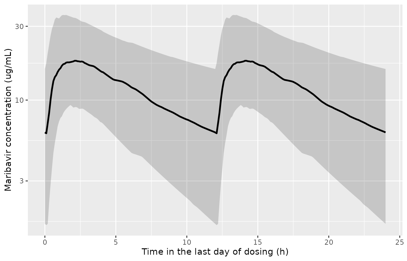
Simulated steady-state maribavir profiles over the last day of 400 mg twice daily in transplant recipients with CMV (median and 5th-95th percentiles).
PKNCA validation
Two intervals per subject: the last 12 h dosing interval (228-240 h)
for the Table 3 comparison, and the whole last day (216-240 h) for the
24 h AUCss the exposure-response models consume.
conc_data <- sim_pk |>
  dplyr::filter(!is.na(Cc)) |>
  dplyr::select(id, treatment, time, Cc)

dose_data <- tibble::tibble(
  id = rep(cohort$id, each = 2),
  treatment = "400 mg BID",
  time = rep(c(216, 228), times = n_sub),
  dose = 400
)

o_conc <- PKNCA::PKNCAconc(conc_data, Cc ~ time | treatment + id)
o_dose <- PKNCA::PKNCAdose(dose_data, dose ~ time | treatment + id)

intervals <- data.frame(
  start = c(228, 216), end = c(240, 240),
  auclast = TRUE, cmax = c(TRUE, FALSE), cmin = c(TRUE, FALSE)
)

o_nca <- PKNCA::pk.nca(PKNCA::PKNCAdata(o_conc, o_dose, intervals = intervals))
nca_res <- as.data.frame(o_nca)

stopifnot(nrow(nca_res) > 0L, !anyNA(nca_res$PPORRES))

nca_tau <- dplyr::filter(nca_res, start == 228)
nca_day <- dplyr::filter(nca_res, start == 216, PPTESTCD == "auclast")
Comparison against published NCA
Song 2024 Table 3 reports geometric mean (CV%) steady-state exposure
at 400 mg twice daily for the 253 SOLSTICE refractory patients with PK,
from post-hoc individual estimates: AUC0-tau 129 ug*h/mL
(51.6%), Cmax,ss 16.9 ug/mL (39.1%),
Ctrough,ss 5.13 ug/mL (93.0%).
reference <- tibble::tribble(
  ~treatment,    ~PPTESTCD, ~PPORRES,
  "400 mg BID",  "auclast",   129,
  "400 mg BID",  "cmax",       16.9,
  "400 mg BID",  "cmin",        5.13
)

nlmixr2lib::ncaComparisonTable(
  simulated = nca_tau,
  reference = reference,
  by = "treatment",
  params = c(
    "AUC0-tau (ug*h/mL)" = "auclast",
    "Cmax,ss (ug/mL)" = "cmax",
    "Ctrough,ss (ug/mL)" = "cmin"
  ),
  label_first_column = "NCA parameter"
) |>
knitr::kable(caption = "Simulated versus Song 2024 Table 3 (SOLSTICE refractory) steady-state exposure. Values marked with a star differ by more than 20%.")| NCA parameter | treatment | Reference | Simulated | % diff |
|---|---|---|---|---|
| Cmax | 400 mg BID | 16.9 | 18.8 | +11.3% |
| Cmin | 400 mg BID | 5.13 | 5.95 | +16.0% |
| AUClast | 400 mg BID | 129 | 142 | +9.7% |
gm_check <- nca_tau |>
  dplyr::filter(PPTESTCD %in% c("auclast", "cmax", "cmin")) |>
  dplyr::group_by(PPTESTCD) |>
  dplyr::summarise(
    gm = exp(mean(log(PPORRES))),
    cv = 100 * sqrt(exp(stats::var(log(PPORRES))) - 1),
    .groups = "drop"
  ) |>
  dplyr::inner_join(reference, by = "PPTESTCD") |>
  dplyr::mutate(pct_diff = 100 * (gm - PPORRES) / PPORRES)

gm_check |>
  dplyr::mutate(dplyr::across(where(is.numeric), \(x) round(x, 2))) |>
  dplyr::select(PPTESTCD, simulated_gm = gm, simulated_cv = cv,
                published_gm = PPORRES, pct_diff) |>
knitr::kable(caption = "Geometric means, the statistic Table 3 reports.")| PPTESTCD | simulated_gm | simulated_cv | published_gm | pct_diff |
|---|---|---|---|---|
| auclast | 139.43 | 54.27 | 129.00 | 8.08 |
| cmax | 18.88 | 44.17 | 16.90 | 11.72 |
| cmin | 5.52 | 94.14 | 5.13 | 7.59 |
stopifnot(
  # AUC and Cmax are set by CL/F and Vc/F, the best-determined parameters; a
  # mis-transcribed PK model moves them by tens of percent.
  max(abs(gm_check$pct_diff[gm_check$PPTESTCD %in% c("auclast", "cmax")])) < 15,
  # The trough is absorption- and lag-driven and the most variable metric.
  abs(gm_check$pct_diff[gm_check$PPTESTCD == "cmin"]) < 30
)

# The 24 h AUC is the sum of two identical steady-state intervals.
day_ratio <- stats::median(
  nca_day$PPORRES /
    nca_tau$PPORRES[nca_tau$PPTESTCD == "auclast"][match(nca_day$id, nca_tau$id[nca_tau$PPTESTCD == "auclast"])]
)
day_ratio
#> [1] 1.999999
stopifnot(abs(day_ratio - 2) < 0.01)
All three simulated geometric means sit within about 12% of Table 3 and on the high side. Two differences in the comparison are expected to contribute: the simulated cohort carries no concomitant medication, whereas Table 3 includes patients on strong CYP3A inhibitors or inducers, and Table 3 summarises post-hoc estimates that are shrunk toward the typical value rather than prospective draws from the full IIV. The gates above allow 15% for AUC and Cmax and 30% for the much more variable trough.
The ratio check is the one that matters for the exposure-response
models: the 24 h AUCss they consume is exactly twice the
dosing-interval AUC. Song 2024’s own numbers agree – Table 3’s
AUC0-tau geometric mean of 129 ug*h/mL is consistent with
the median AUCss of about 238 ug*h/mL printed in Figure
S1.5.
Exposure-response: end to end
The simulated exposures and risk factors are now fed through all six models.
expo <- nca_tau |>
  dplyr::filter(PPTESTCD %in% c("cmax", "cmin")) |>
  dplyr::select(id, PPTESTCD, PPORRES) |>
  tidyr::pivot_wider(names_from = PPTESTCD, values_from = PPORRES) |>
  dplyr::rename(CMAX = cmax, CTROUGH = cmin) |>
  dplyr::left_join(
    dplyr::transmute(nca_day, id, AUC_MBV_SS24 = PPORRES),
    by = "id"
  ) |>
  dplyr::mutate(CAV = AUC_MBV_SS24 / 24)

er_data <- dplyr::left_join(cohort, expo, by = "id")

predict_er <- function(nm, data) {
  ui <- er_ui[[nm]]
  ev <- data.frame(id = data$id, time = 0, evid = 0L, amt = NA_real_, dv = NA_real_)
  for (cv in ui$allCovs) ev[[cv]] <- data[[cv]]
  out <- rxode2::rxSolve(rxode2::zeroRe(ui), ev, returnType = "data.frame")
  out[[grep("^prob_", names(out), value = TRUE)[1]]]
}

er_pred <- lapply(er_models, predict_er, data = er_data)
#> Warning: No omega parameters in the model
#> Warning: multi-subject simulation without without 'omega'
#> Warning: No omega parameters in the model
#> Warning: multi-subject simulation without without 'omega'
#> Warning: No omega parameters in the model
#> Warning: multi-subject simulation without without 'omega'
#> Warning: No omega parameters in the model
#> Warning: multi-subject simulation without without 'omega'
#> Warning: No omega parameters in the model
#> Warning: multi-subject simulation without without 'omega'
#> Warning: No omega parameters in the model
#> Warning: multi-subject simulation without without 'omega'
names(er_pred) <- er_models

stopifnot(all(vapply(er_pred, function(p) all(p > 0 & p < 1), logical(1))))

expo |>
  dplyr::summarise(dplyr::across(c(AUC_MBV_SS24, CTROUGH, CMAX, CAV),
                                 \(x) round(stats::median(x), 2))) |>
knitr::kable(caption = "Median simulated exposure columns (Figure S1.5 median AUCss about 238 ug*h/mL; Figure S1.3 median Cavg about 10.6 ug/mL; Figure S1.4 median Cmax,ss about 17.6 ug/mL).")| AUC_MBV_SS24 | CTROUGH | CMAX | CAV |
|---|---|---|---|
| 283.13 | 5.95 | 18.8 | 11.8 |
The simulated medians run above the figure medians, in line with the Table 3 comparison above; the exposure-response analysis set is also not identical to the 253-patient Table 3 set.
Mean-probability identity
For a logistic regression fitted by maximum likelihood with an intercept, the mean fitted probability over the analysis set equals the observed event rate. The simulated cohort is not the analysis set – its covariates are drawn independently from published marginals, and its exposures are prospective rather than post-hoc – so the identity holds only approximately. It is still a sharp check on the coefficient scale: a slope off by a factor of 50, an exposure column off by a factor of 2, or an uncentred term that should have been centred moves the mean probability by far more than these approximations do. For the digitised safety models it is a check made with numbers the digitisation never used.
identity <- tibble::tibble(
  Model = sub("^Song_2024_maribavir_", "", er_models),
  Observed = c(131, 44, 60, 88, 108, 28) / 231,
  `Mean predicted` = vapply(er_pred, mean, numeric(1))
) |>
  dplyr::mutate(Difference = `Mean predicted` - Observed)

knitr::kable(identity, digits = 3,
caption = "Mean predicted probability over the simulated cohort against the observed event rate in the 231-patient analysis set.")| Model | Observed | Mean predicted | Difference |
|---|---|---|---|
| cmv_clearance_wk8 | 0.567 | 0.553 | -0.014 |
| cmv_clearance_wk16 | 0.190 | 0.166 | -0.024 |
| te_resistance | 0.260 | 0.269 | 0.009 |
| sae | 0.381 | 0.412 | 0.031 |
| dysgeusia | 0.468 | 0.445 | -0.022 |
| fatigue | 0.121 | 0.138 | 0.017 |
Two encoding choices rest on this identity. Table 6 enters age
uncentred: with an age term centred at the median of 56
years, the mean predicted probability of resistance would be about 0.6
against an observed 0.26. And the efficacy models need the 24
h AUC: supplying the 12 h AUC0-tau instead would
lift the predicted week-16 response rate well above the observed
19%.
p_age_centred <- mean(stats::plogis(
  qlogis(er_pred[[res]]) - er_ini(res)[["e_age_logit"]] * 56
))
p_auc_tau <- mean(predict_er(wk16, dplyr::mutate(er_data, AUC_MBV_SS24 = AUC_MBV_SS24 / 2)))
#> Warning: No omega parameters in the model
#> Warning: multi-subject simulation without without 'omega'
c(age_centred_resistance = p_age_centred, wk16_with_auc_tau = p_auc_tau)
#> age_centred_resistance      wk16_with_auc_tau
#>              0.6088976              0.2760194
stopifnot(
  abs(p_age_centred - 60 / 231) > 0.2,
  p_auc_tau - 44 / 231 > 0.05
)
Exposure-response curves
auc_grid <- seq(72, 802, length.out = 100)
curve_eff <- dplyr::bind_rows(lapply(c(wk8, wk16), function(nm) {
  te_col <- if (nm == wk8) "TE_RESIST_MBV_ONTX" else "TE_RESIST_MBV"
  dplyr::bind_rows(lapply(0:1, function(te) {
    d <- data.frame(id = seq_along(auc_grid), AUC_MBV_SS24 = auc_grid)
    for (cv in setdiff(er_ui[[nm]]$allCovs, "AUC_MBV_SS24")) d[[cv]] <- 0
    d[[te_col]] <- te
    data.frame(
      endpoint = if (nm == wk8) "Week 8 (primary)" else "Week 16 maintained (key secondary)",
      resistance = if (te == 1) "TE resistance mutation" else "No TE resistance",
      AUC = auc_grid, p = predict_er(nm, d)
    )
  }))
}))
#> Warning: No omega parameters in the model
#> Warning: multi-subject simulation without without 'omega'
#> Warning: No omega parameters in the model
#> Warning: multi-subject simulation without without 'omega'
#> Warning: No omega parameters in the model
#> Warning: multi-subject simulation without without 'omega'
#> Warning: No omega parameters in the model
#> Warning: multi-subject simulation without without 'omega'
ggplot2::ggplot(curve_eff, ggplot2::aes(AUC, p, linetype = resistance)) +
  ggplot2::geom_line() +
  ggplot2::facet_wrap(~endpoint) +
  ggplot2::coord_cartesian(ylim = c(0, 1)) +
  ggplot2::labs(x = "AUCss, 0-24 h (ug*h/mL)", y = "Probability of response", linetype = NULL) +
  ggplot2::theme(legend.position = "bottom")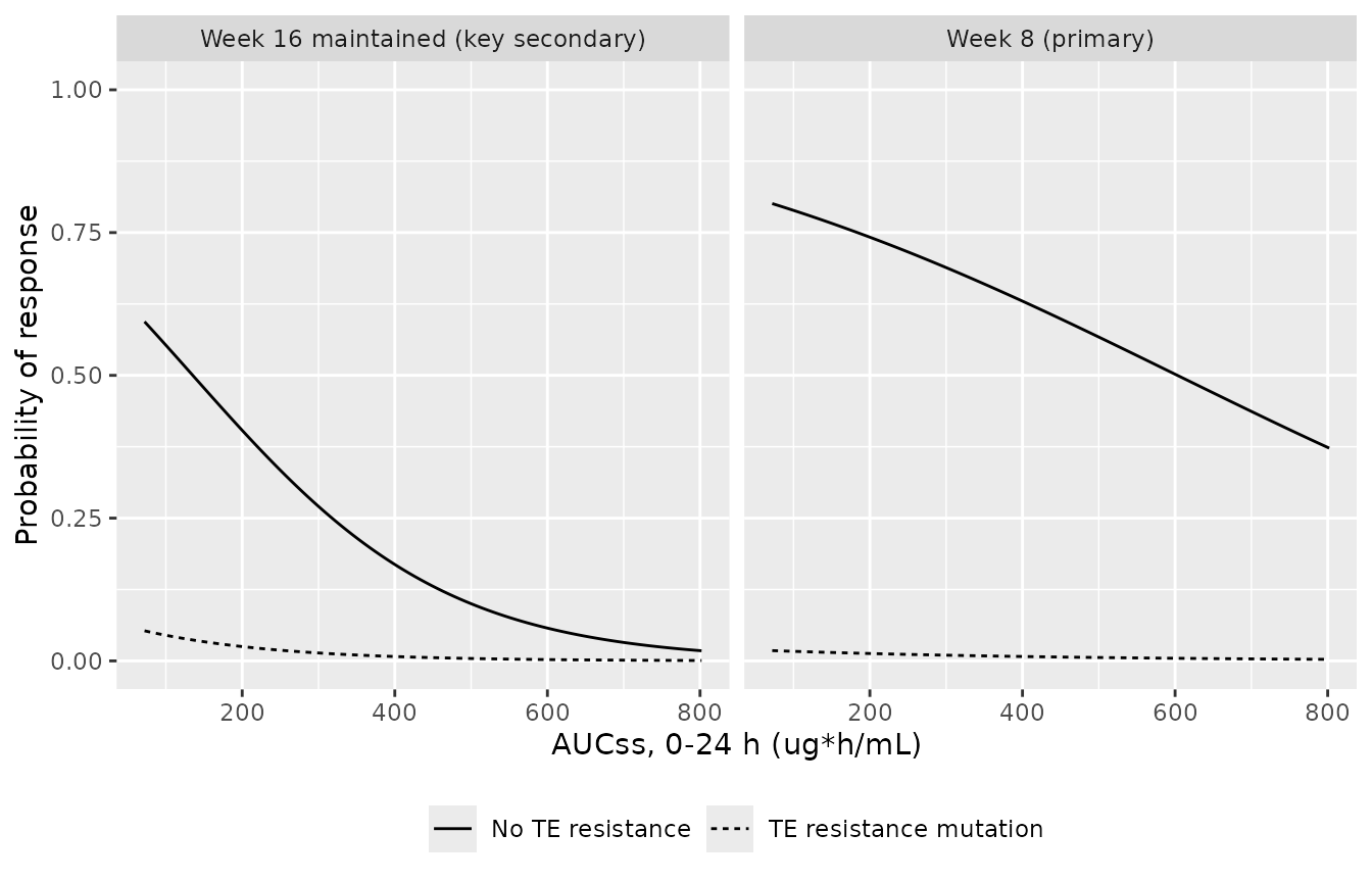
Primary (Table 5) and key secondary (Table S1.3) endpoints against the 0-24 h steady-state AUC for the reference patient (no resistance mutation, CD8+CD69+ < 0.5%, low CMV DNA, no prior prophylaxis), with the effect of a treatment-emergent resistance mutation. Song 2024 Figure 4 and Figure S1.2 show the exposure-only fits for the same endpoints; the curves here are the final multivariable models.
ct_grid <- seq(0.5, 20, length.out = 100)
curve_res <- dplyr::bind_rows(lapply(c("low", "int", "high"), function(lvl) {
  d <- data.frame(id = seq_along(ct_grid), CTROUGH = ct_grid)
  for (cv in setdiff(er_ui[[res]]$allCovs, "CTROUGH")) d[[cv]] <- 0
  d$AGE <- 56
  d$TX_HCT <- 1
  d$CMVDNA_HIGH <- as.integer(lvl != "low")
  d$CMVDNA_VHIGH <- as.integer(lvl == "high")
  data.frame(cmvdna = lvl, Ctrough = ct_grid, p = predict_er(res, d))
}))
#> Warning: No omega parameters in the model
#> Warning: multi-subject simulation without without 'omega'
#> Warning: No omega parameters in the model
#> Warning: multi-subject simulation without without 'omega'
#> Warning: No omega parameters in the model
#> Warning: multi-subject simulation without without 'omega'
curve_res$cmvdna <- factor(curve_res$cmvdna, c("low", "int", "high"),
                           c("Low (< 9100 IU/mL)", "Intermediate", "High (>= 91 000 IU/mL)"))
ggplot2::ggplot(curve_res, ggplot2::aes(Ctrough, p, colour = cmvdna)) +
  ggplot2::geom_line(linewidth = 1) +
  ggplot2::coord_cartesian(ylim = c(0, 1)) +
  ggplot2::labs(x = "Ctrough,ss (ug/mL)", y = "Probability of TE resistance",
                colour = "Baseline CMV DNA") +
  ggplot2::theme(legend.position = "bottom")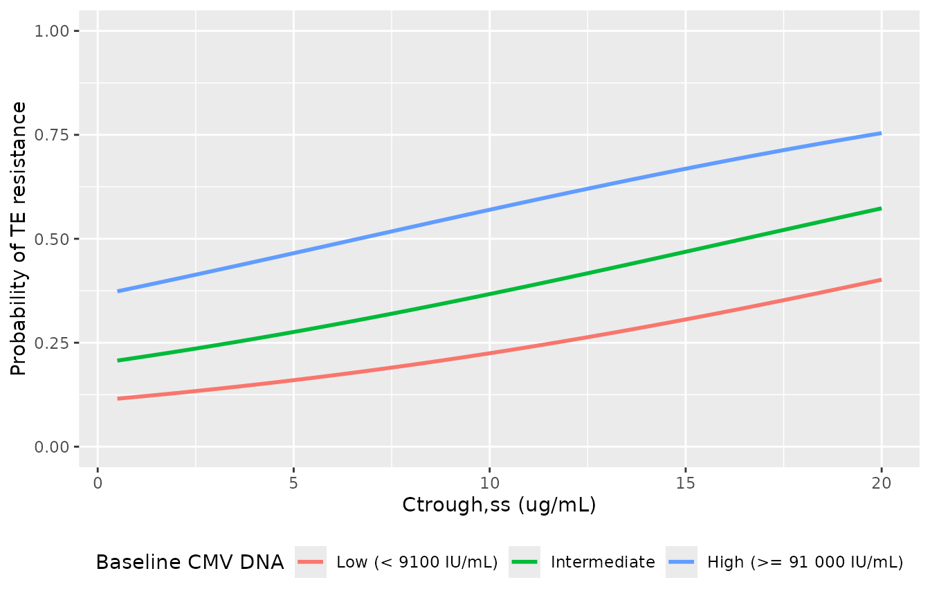
Probability of a treatment-emergent maribavir-resistant mutation (Table 6) against steady-state trough concentration, by baseline CMV DNA, for a 56-year-old HCT recipient without baseline resistance and CD4+CD69+ < 0.5%. Compare with Song 2024 Figure 5, which shows the exposure-only fit.
quart <- tibble::tribble(
  ~endpoint,       ~lo,  ~hi,   ~obs,  ~lcl,  ~ucl,
  "sae",           72.2, 170,   0.293, 0.181, 0.427,
  "sae",           170,  238,   0.351, 0.229, 0.489,
  "sae",           238,  354,   0.345, 0.225, 0.481,
  "sae",           354,  802,   0.534, 0.399, 0.667,
  "dysgeusia",     3.50, 7.83,  0.534, 0.399, 0.667,
  "dysgeusia",     7.83, 10.6,  0.579, 0.441, 0.709,
  "dysgeusia",     10.6, 14.6,  0.448, 0.317, 0.585,
  "dysgeusia",     14.6, 38.3,  0.310, 0.195, 0.445,
  "fatigue",       7.37, 12.9,  0.052, 0.011, 0.144,
  "fatigue",       12.9, 17.6,  0.088, 0.029, 0.193,
  "fatigue",       17.6, 22.6,  0.086, 0.029, 0.190,
  "fatigue",       22.6, 47.0,  0.259, 0.153, 0.390
) |>
  dplyr::mutate(x = (lo + hi) / 2)

saf <- c(sae = "AUC_MBV_SS24", dysgeusia = "CAV", fatigue = "CMAX")
curve_saf <- dplyr::bind_rows(lapply(names(saf), function(ep) {
  rng <- range(quart$lo[quart$endpoint == ep], quart$hi[quart$endpoint == ep])
  x <- seq(rng[1], rng[2], length.out = 100)
  d <- data.frame(id = seq_along(x))
  d[[saf[[ep]]]] <- x
  data.frame(endpoint = ep, x = x, p = predict_er(paste0("Song_2024_maribavir_", ep), d))
}))
#> Warning: No omega parameters in the model
#> Warning: multi-subject simulation without without 'omega'
#> Warning: No omega parameters in the model
#> Warning: multi-subject simulation without without 'omega'
#> Warning: No omega parameters in the model
#> Warning: multi-subject simulation without without 'omega'
ggplot2::ggplot() +
  ggplot2::geom_line(data = curve_saf, ggplot2::aes(x, p)) +
  ggplot2::geom_pointrange(data = quart, ggplot2::aes(x, obs, ymin = lcl, ymax = ucl)) +
  ggplot2::facet_wrap(~endpoint, scales = "free_x",
                      labeller = ggplot2::labeller(endpoint = c(
                        sae = "Serious AE vs AUCss (ug*h/mL)",
                        dysgeusia = "Taste disturbance vs Cavg (ug/mL)",
                        fatigue = "Fatigue vs Cmax,ss (ug/mL)"))) +
  ggplot2::coord_cartesian(ylim = c(0, 1)) +
  ggplot2::labs(x = NULL, y = "Probability")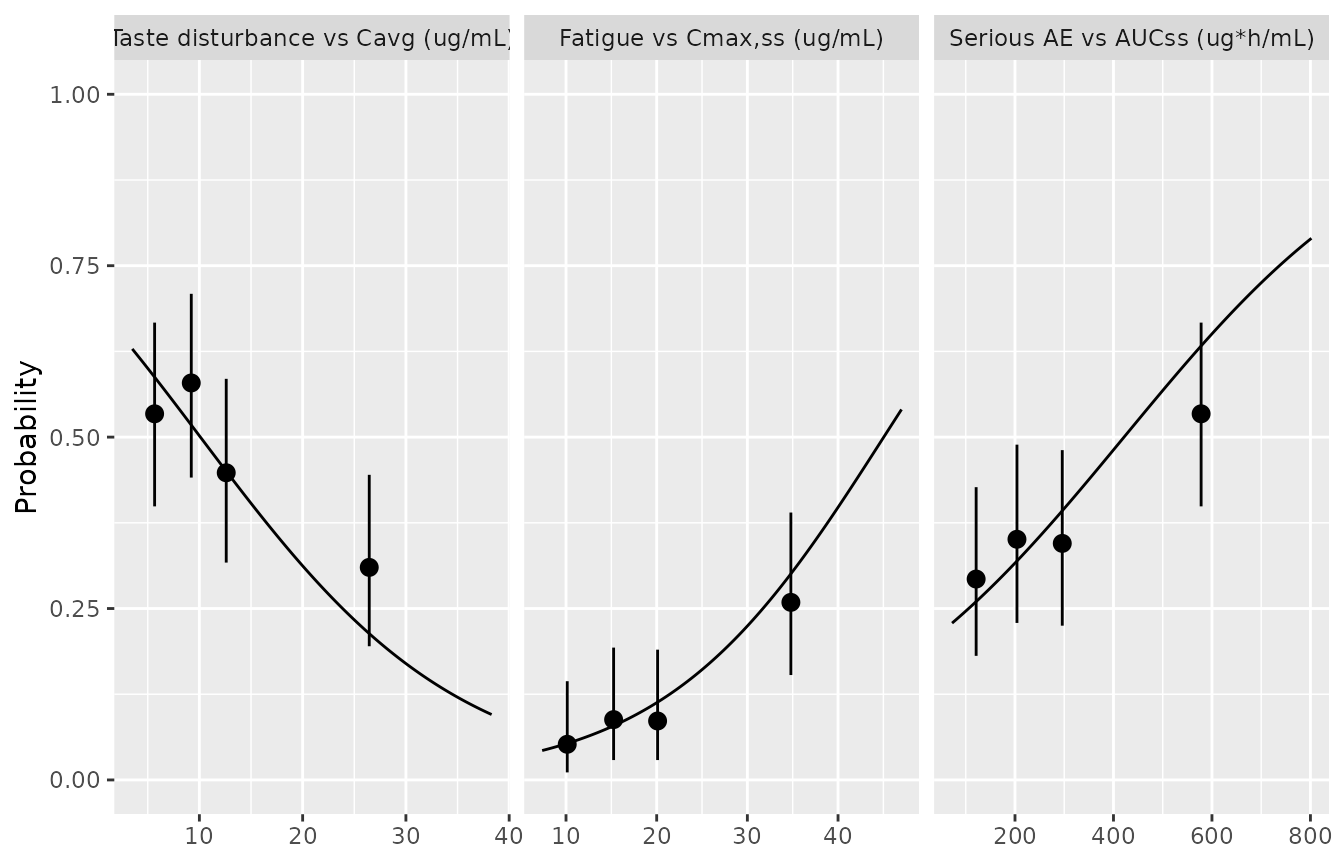
Replicates Song 2024 Figures S1.3-S1.5: the packaged safety models (lines) against the observed event proportions and 95% CIs in each exposure quartile, as printed beneath each figure (points at the quartile mid-range).
Assumptions and deviations
The PK model is not repackaged
Song 2024’s final popPK model is the NONMEM run already packaged as
Sun_2023_maribavir, and its Table 2 reproduces that file to
within rounding. The Song 2024 supplement prints only the
initial $THETA / $OMEGA estimates of
that run, so the existing file – whose source carried the converged
values and the full OMEGA block – is the better-sourced copy.
The three safety models are digitised, univariate fits
- Coefficients recovered from figures. Song 2024 prints no coefficient table for the taste-disturbance, fatigue and serious-adverse-event models, only the fitted curves in Supplementary Figures S1.3-S1.5 with their p-values. The intercepts and slopes were digitised by the maintainers as described in the Source trace, and are rounded to four significant figures. Treat them as reproductions of the plotted curves, not as published estimates.
-
They are the exposure-only fits. The paper’s final
safety models also retained other risk factors – transplant type and
enrolment region for taste disturbance, enrolment region for fatigue,
baseline CMV resistance and baseline CMV DNA for serious adverse events
– whose coefficients are not reported. The figures draw the
exposure-only regression, and that is what is packaged. The unreported
terms are recorded in each file’s
covariatesDataExcludedor covariate notes. -
Cavg is per patient. Song 2024 defines Cavg as the
“average concentration on each study day” and plots one value per
patient, without saying how the days were summarised. At steady state
the daily average is
AUCss / 24, which is what this vignette supplies.
Covariate encoding
-
Two nested CMV DNA indicators.
CMVDNA_HIGHmarks>= 9100 IU/mLandCMVDNA_VHIGHmarks>= 91 000 IU/mL, so Table 6’s three levels areCMVDNA_HIGH - CMVDNA_VHIGH(intermediate) andCMVDNA_VHIGH(high), and Table S1.3’s pooled “intermediate/high” isCMVDNA_HIGH. Song 2024 does not print the cut-points; they come from the SOLSTICE primary publication (Avery 2022). Note that the Sun 2025 AURORA paper calls>= 9100 IU/mL“high”: the same word names different cut-points in the two trials. -
Two nested resistance indicators. The
primary-endpoint model uses a mutation detected during
treatment (
TE_RESIST_MBV_ONTX, 47 patients), the key-secondary model a mutation detected at any time (TE_RESIST_MBV, 60). Both are on-study outcomes used as predictors of another on-study outcome, so these coefficients describe association, not baseline prognosis. -
Solid organ transplant as
1 - TX_HCT. Exact for this cohort of 140 SOT and 91 HCT recipients with no non-transplant subject. -
Not reported is a fitted level.
CD8_PP65_NR/CD4_PP65_NRcarry their own coefficients. A result reported as “too few cells for analysis” is not “not reported”: Table S1.2 footnote a assigns it to the< 0.5%reference. - Baseline CMV resistance, 5 unreported. The paper does not say how the 5 patients with unreported baseline resistance were coded.
Source discrepancies
-
One printed odds ratio disagrees with its estimate.
Table 5 prints
-0.304with odds ratio0.739for the CD8+CD69+>= 0.5% to < 2%stratum, butexp(-0.304) = 0.738, and no estimate that rounds to-0.304gives an odds ratio that rounds to0.739. The other twenty printed odds ratios agree with their estimates. The packaged value is the printed estimate; the difference is far below the coefficient’s standard error (0.492). -
One Results-text probability does not reproduce.
The Table 5 profile with CD8+CD69+
>= 2%is quoted as 90.0%; the printed coefficients give 90.4%, and no values inside their rounding intervals reach 90.0%. The other thirteen quoted probabilities reproduce to their printed precision, so the transcription is not in doubt; the 0.4-point gap is in the source text. - Table 6 scenarios evaluate the age term at zero. The Results quote probabilities “of the same age” – 54.5% for the reference patient, for example – that reproduce only with the age term omitted. Age is nonetheless uncentred in the model, as the mean-probability identity above confirms.
- Table 4 age band. The first age band of Table 4 is printed “18 to < 65”; the counts and the next band (“45 to < 65”) show it is 18 to < 45.
- A units slip. The Results quote the Table 6 scenarios at “Ctrough,ss of 5 ug*h/mL”; a trough is a concentration, and 5 ug/mL is used.
Simulation assumptions
- Independent covariates. The virtual cohort draws each risk factor independently from its published marginal, except that the CD4 and CD8 assays share their 46 unreported patients. The real covariates are correlated – above all, the treatment-emergent resistance mutation is more common at high exposure – so the cohort reproduces the overall event rates only approximately.
- Prospective, not post-hoc, exposures, and no concomitant medication. The source exposures are empirical-Bayes predictions with the actual dosing history and strong CYP3A inhibitor / inducer use.
-
Placeholder residual error. Every model carries
addSd_prob_* <- fixed(0.001)only so rxode2 has an error model to attach to the probability; the source likelihood is Bernoulli and has no residual error. The vignette solves the models withzeroRe().