Valbenazine popPK + chorea exposure-efficacy (Nguyen 2025)
Source:vignettes/articles/Nguyen_2025_valbenazine_huntington_chorea.Rmd
Nguyen_2025_valbenazine_huntington_chorea.RmdModel and source
Nguyen 2025 reports two models, fitted sequentially, and this paper therefore contributes two model files to nlmixr2lib:
| Model file | Role |
|---|---|
Nguyen_2025_valbenazine |
Joint parent-metabolite population PK of valbenazine and
[+]-alpha-HTBZ |
Nguyen_2025_valbenazine_tmc |
Longitudinal exposure-efficacy model of the change from baseline in Total Maximal Chorea (TMC) score |
The link between them is one-directional and explicit: the PK model
generates Bayesian post-hoc daily [+]-alpha-HTBZ AUC
values, and those AUC values are the sole exposure driver of the
efficacy model. The paper calls this a sequential E-R analysis;
the two fits do not share random effects.
- Article: https://doi.org/10.1002/jcph.70092
- Supplement: published with the open-access article, PMC12649288
(
JCPH-65-1777-s001.pdf)
#> ℹ parameter labels from comments will be replaced by 'label()'
#> ℹ parameter labels from comments will be replaced by 'label()'- Citation: Nguyen HQ, Crass RL, Chapel S, Kuan HYS, Loewen G, Brar S. Population pharmacokinetic and exposure-efficacy analyses of valbenazine in patients with Huntington’s disease: supporting dose selection for chorea management. The Journal of Clinical Pharmacology. 2025;65(12):1777-1788. doi:10.1002/jcph.70092. Parameter estimates from Table 1; covariate-parameter equations from Supplemental Table S2; individual empirical Bayes parameter distributions from Supplemental Table S3. Companion exposure-efficacy model from the same paper: modellib(‘Nguyen_2025_valbenazine_tmc’).
PK model. Joint parent-metabolite population pharmacokinetic model of valbenazine and its active metabolite [+]-alpha-dihydrotetrabenazine ([+]-alpha-HTBZ, NBI-98782) in healthy adults and in patients with tardive dyskinesia or Huntington’s disease chorea (Nguyen 2025). Valbenazine is absorbed through a chain of four transit compartments (transit rate constant KTR = KA) into a two-compartment linear disposition system; a fraction FM = 0.207 of the valbenazine elimination flux forms [+]-alpha-HTBZ, which itself follows two-compartment linear disposition. The two analytes SHARE the apparent central volume VC/F – the identifiability constraint that makes FM estimable (previously fixed at 0.35 in the predecessor model). Relative bioavailability rises saturably with dose (Emax form anchored at the 1 mg dose, FMAX = 1.36, ED50 = 90.1 mg); the effect is small at clinically relevant doses (1.09- and 1.16-fold at 60 and 80 mg relative to 40 mg). Covariates: allometric body weight on CLP/F and VC/F (70 kg reference), oral-solution formulation and fed state on KTR, fed state on F1, and CYP2D6 poor- and intermediate-metabolizer status on the metabolite clearance CLM (51.6% and 28.1% reductions relative to extensive or ultra-rapid metabolizers). Residual error is log-additive and stratified by analyte and by sampling design (intensive vs sparse), switched per observation record through SAMPLE_INTENSIVE.
E-R model. Longitudinal exposure-efficacy model of the change from baseline in the UHDRS Total Maximal Chorea (TMC) score under valbenazine in adults with Huntington’s-disease chorea (Nguyen 2025, KINECT-HD). The response is DECOUPLED: a time-dependent placebo term applies only to placebo-arm subjects, and a nonlinear Emax term in the daily [+]-alpha-dihydrotetrabenazine ([+]-alpha-HTBZ) AUC applies to everyone. The placebo term is an asymptotic exponential onset, 1 - exp(-KPBO * t), with an onset half-life of 9.18 days, multiplied after day TATT = 59 by an attenuation factor exp(-KATT * (t - TATT)) with an attenuation half-life of 36.4 days – reproducing the observed placebo response that peaks near week 8 and then returns toward baseline. The drug term is Emax * AUC / (EC50 + AUC) with Emax = -14.2 TMC points and EC50 = exp(7.50) ng*h/mL. Inter-individual variability is ADDITIVE on Pmax and log-normal on EC50 (125% CV), and the residual error is additive on the TMC scale. The model has NO ODE states and no dosing: it is an algebraic function of study time, the placebo-arm indicator, and the exposure covariate AUC_HTBZ, which must be supplied per observation record – typically from the companion population PK model, modellib(‘Nguyen_2025_valbenazine’).
Population
The population PK analysis pooled 8 studies / 425
subjects contributing 7279 valbenazine and 7092
[+]-alpha-HTBZ plasma concentration records: six phase 1
studies in healthy adults (1 to 150 mg), the KINECT 3 phase 3 study in
tardive dyskinesia (TD; 40 or 80 mg once daily), and the KINECT-HD phase
3 study in Huntington’s-disease chorea (HD; 40 to 80 mg once daily).
Mean (SD) age was 48.3 (14.3) years and mean (SD) body weight 77.8
(15.7) kg, with 43.3% female. CYP2D6 phenotype was 58.2% extensive,
30.5% intermediate, 5.6% poor and 3.2% ultra-rapid metabolizers (Nguyen
2025 Results).
The exposure-efficacy analysis used KINECT-HD only: 125 subjects (61 placebo, 64 valbenazine) contributing 937 TMC assessments including 125 baseline assessments. That cohort was 54.4% female, 96.0% White, median age 55.0 years (range 25-74) and median weight 75.8 kg (range 41.0-134) – Supplemental Tables S5 and S6. Dosing began at 40 mg once daily and could escalate in 20 mg increments at the end of weeks 2, 4 and 6 to a target of 80 mg once daily; by week 12, 45 of 57 valbenazine subjects were at 80 mg, which is why the observed means at 20 and 40 mg in Table 4 rest on one to three subjects.
Both models carry this information programmatically:
str(pk$population,  max.level = 1, give.attr = FALSE)
#> List of 13
#>  $ species       : chr "human"
#>  $ n_subjects    : int 425
#>  $ n_studies     : int 8
#>  $ n_observations: int 14371
#>  $ age_range     : chr "mean (SD) 48.3 (14.3) years across the pooled PK dataset; KINECT-HD enrolled adults 18-75 years"
#>  $ weight_range  : chr "mean (SD) 77.8 (15.7) kg across the pooled PK dataset; KINECT-HD 41.0-134 kg (median 75.8)"
#>  $ weight_median : chr "75.8 kg (KINECT-HD full analysis set, Supplemental Table S6)"
#>  $ sex_female_pct: num 43.3
#>  $ race_ethnicity: Named num [1:4] 96 0.8 0.8 2.4
#>  $ disease_state : chr "Pooled: healthy adults (six phase 1 studies), patients with tardive dyskinesia (KINECT 3, NCT02274558), and pat"| __truncated__
#>  $ dose_range    : chr "1-150 mg valbenazine orally in the phase 1 studies; 40-80 mg once daily in KINECT-HD; 40 or 80 mg once daily in KINECT 3"
#>  $ cyp2d6_status : Named num [1:4] 58.2 30.5 5.6 3.2
#>  $ notes         : chr "Pooled PK analysis dataset: 7279 valbenazine and 7092 [+]-alpha-HTBZ plasma concentration records from 425 pati"| __truncated__
str(tmc$population, max.level = 1, give.attr = FALSE)
#> List of 15
#>  $ species       : chr "human"
#>  $ n_subjects    : int 125
#>  $ n_studies     : int 1
#>  $ n_observations: int 937
#>  $ age_range     : chr "25-74 years (mean (SD) 53.7 (10.8); median 55.0)"
#>  $ age_median    : chr "55.0 years"
#>  $ weight_range  : chr "41.0-134 kg (mean (SD) 77.0 (18.0); median 75.8)"
#>  $ weight_median : chr "75.8 kg"
#>  $ sex_female_pct: num 54.4
#>  $ race_ethnicity: Named num [1:4] 96 0.8 0.8 2.4
#>  $ hispanic_pct  : num 6.4
#>  $ disease_state : chr "Adults with chorea associated with Huntington's disease (KINECT-HD, protocol HD3005; a phase 3 randomized doubl"| __truncated__
#>  $ dose_range    : chr "Placebo, or valbenazine titrated from 40 mg once daily in 20 mg increments at the end of weeks 2, 4 and 6 to a "| __truncated__
#>  $ cyp2d6_status : Named num [1:5] 48 37.6 7.2 4.8 2.4
#>  $ notes         : chr "128 subjects received study treatment (64 placebo, 64 valbenazine); three placebo subjects had no post-treatmen"| __truncated__
Source trace
Per-parameter provenance is recorded as an in-file comment beside
each ini() entry in
inst/modeldb/specificDrugs/Nguyen_2025_valbenazine.R and
inst/modeldb/specificDrugs/Nguyen_2025_valbenazine_tmc.R.
Collected here for review.
Population PK model
| Equation / parameter | Value | Source location |
|---|---|---|
lcl (CLP/F) |
23.2 L/h | Table 1 theta 1 |
lvc (VC/F, shared) |
226 L | Table 1 theta 2 |
lktr (KA = KTR) |
8.43 1/h | Table 1 theta 3 |
lq (QP/F) |
22.0 L/h | Table 1 theta 4 |
lvp (VPP/F) |
198 L | Table 1 theta 5 |
lfmax (FMAX) |
1.36 | Table 1 theta 6 |
led50 (ED50) |
90.1 mg | Table 1 theta 7 |
e_soln_ktr |
1.51 | Table 1 theta 8 |
e_fed_ktr |
-0.685 | Table 1 theta 9 |
e_fed_fdepot |
-0.0646 | Table 1 theta 10 |
lcl_htbz (CLM) |
31.0 L/h | Table 1 theta 13 |
fm (FM) |
0.207 | Table 1 theta 14 |
lq_htbz (QM) |
1.27 L/h | Table 1 theta 15 |
lvp_htbz (VPM) |
97.8 L | Table 1 theta 16 |
e_cyp2d6_pm_cl_htbz |
-0.516 | Table 1 theta 17 |
e_cyp2d6_im_cl_htbz |
-0.281 | Table 1 theta 18 |
e_wt_cl |
0.602 | Table 1 theta 21 |
e_wt_vc |
1.04 | Table 1 theta 22 |
expSdIntensive / expSdSparse
|
0.402 / 0.678 | Table 1 thetas 11, 12 |
expSdIntensive_htbz /
expSdSparse_htbz
|
0.264 / 0.720 | Table 1 thetas 19, 20 |
| IIV omega-squared on CLP/F, VC/F, KA, CLM | 0.150, 0.194, 0.187, 0.225 | Table 1 IIV block |
CLP/F equation, (WT/70)^exponent
|
n/a | Supplemental Table S2 eq (1) |
VC/F equation, (WT/70)^exponent
|
n/a | Supplemental Table S2 eq (2) |
KTR equation, (1 + t8*SOLN)(1 + t9*FED)
|
n/a | Supplemental Table S2 eq (3) |
F1 equation,
[1 + FMAX*(DOSE-1)/(ED50+DOSE-1)](1 + t10*FED)
|
n/a | Supplemental Table S2 eq (4) |
CLM equation, (1 + t17*PM)(1 + t18*IM)
|
n/a | Supplemental Table S2 eq (5) |
| Four transit absorption compartments; KA = KTR | n/a | Results, “Population PK Model Development”; Table S2 eq (3) |
| Shared VC/F constraint identifying FM | n/a | Methods, “Population PK Modeling” |
| 70 kg reference weight | n/a | Supplemental Table S2 parameter definitions |
MW valbenazine 418.57, MW [+]-alpha-HTBZ 319.44 |
g/mol | Not from the paper – see Assumptions |
Exposure-efficacy model
| Equation / parameter | Value | Source location |
|---|---|---|
pmax (Pmax) |
-2.35 TMC points | Table 3 theta 1 |
lthalf_onset (HLPLB) |
9.18 day | Table 3 theta 2 |
ltswitch (TATT) |
59.0 day | Table 3 theta 3 |
lthalf_att (HLATT) |
36.4 day | Table 3 theta 4 |
emax (Emax) |
-14.2 TMC points | Table 3 theta 5 |
lec50 (log EC50) |
7.50 | Table 3 theta 6 |
addSd |
1.41 TMC points | Table 3 theta 7 (reported as variance 1.98) |
etapmax omega-squared |
5.11 | Table 3 IIV block (SD 2.26) |
etalec50 omega-squared |
0.941 | Table 3 IIV block (125% CV) |
| Placebo equation with attenuation | n/a | Methods, “Exposure-Efficacy Modeling”, eq 1 |
KPBO = 0.693/HLPLB,
KATT = 0.693/HLATT
|
n/a | Methods, “Exposure-Efficacy Modeling”, eq 2 |
R = PBO*PLB + Emax*AUC/(exp(logEC50 + eta) + AUC) |
n/a | Methods, “Exposure-Efficacy Modeling”, eq 3 |
Simulation helpers
Both analytes are ~ endpoints of the PK model, so
observation records carry an explicit dvid; rxode2 returns
both algebraic observables (Cc and
Cc_htbz) as columns on every observation row regardless of
dvid, which is what the checks below read.
The metabolite terminal half-life implied by the model is 57 hours, so a 21-day once-daily run-in is used before the steady-state window (> 8 terminal half-lives). To keep the render cheap the observation grid is coarse during accumulation and dense only over the final dosing interval.
tau  <- 24    # h, once-daily
ndos <- 21    # days of dosing before the steady-state window
ss_start <- tau * (ndos - 1)
ss_end   <- tau * ndos

#' Build a one-subject event table.
#' Observation rows use dvid because the PK model has two `~` endpoints.
make_events <- function(dose_mg, id = 1L, wt = 70, pm = 0, im = 0,
                        fed = 0, soln = 0) {
  dose <- data.frame(
    time = seq(0, ss_start, by = tau), amt = dose_mg,
    evid = 1L, cmt = "depot", dvid = NA_integer_
  )
  obs <- data.frame(
    time = sort(unique(c(seq(0, ss_start, by = 6),
                         seq(ss_start, ss_end, by = 0.1)))),
    amt = NA_real_, evid = 0L, cmt = NA_character_, dvid = 1L
  )
  out <- rbind(dose, obs)
  out <- out[order(out$time, -out$evid), ]
  out$id <- id
  out$WT <- wt
  out$DOSE <- dose_mg
  out$FED <- fed
  out$FORM_SOLUTION <- soln
  out$CYP2D6_PM <- pm
  out$CYP2D6_IM <- im
  out$SAMPLE_INTENSIVE <- 1
  out
}

#' Solve and return the steady-state interval only.
solve_ss <- function(model, events) {
  s <- rxode2::rxSolve(model, events, returnType = "data.frame",
                       useLinCmt = FALSE)
  if (is.null(s$id)) s$id <- 1L
  s[s$time >= ss_start & s$time <= ss_end, ]
}

#' Trapezoidal AUC over a monotone time grid.
auc_trap <- function(time, conc) {
  sum(diff(time) * (utils::head(conc, -1) + utils::tail(conc, -1)) / 2)
}
Gate 1 – closed-form steady-state AUC identity
At steady state the amount of [+]-alpha-HTBZ formed per
dosing interval equals
FM * (MW_HTBZ / MW_valbenazine) * F1(DOSE) * DOSE, and all
of it is cleared by CLM. The metabolite exposure therefore
has an exact closed form independent of every distribution
parameter:
This single identity gates the ODE mass balance, the transit chain,
the molecular-weight conversion, the F1 dose function, the
dose encoding, and PKNCA’s interval settings simultaneously. It must
hold to solver tolerance.
mw_vbz  <- 418.57
mw_htbz <- 319.44
fm      <- 0.207
fmax    <- 1.36
ed50    <- 90.1

f1_of <- function(d, fed = 0) {
  (1 + fmax * pmax(d - 1, 0) / (ed50 + pmax(d - 1, 0))) * (1 + (-0.0646) * fed)
}
closed_form_auc <- function(d, clm, fed = 0) {
  1000 * fm * (mw_htbz / mw_vbz) * f1_of(d, fed) * d / clm
}

# Typical-value model, CLM held at its Table 1 typical value of 31.0 L/h.
pk_typ <- pk |> rxode2::zeroRe()
#> Warning: No sigma parameters in the model

gate1 <- lapply(c(20, 40, 60, 80), function(d) {
  s <- solve_ss(pk_typ, make_events(d))
  data.frame(
    dose        = d,
    ode_auc     = auc_trap(s$time, s$Cc_htbz),
    closed_form = closed_form_auc(d, 31.0)
  )
}) |> bind_rows() |>
  mutate(pct_diff = 100 * (ode_auc - closed_form) / closed_form)
#> ℹ omega/sigma items treated as zero: 'etalcl', 'etalvc', 'etalktr', 'etalcl_htbz'
#> ℹ omega/sigma items treated as zero: 'etalcl', 'etalvc', 'etalktr', 'etalcl_htbz'
#> ℹ omega/sigma items treated as zero: 'etalcl', 'etalvc', 'etalktr', 'etalcl_htbz'
#> ℹ omega/sigma items treated as zero: 'etalcl', 'etalvc', 'etalktr', 'etalcl_htbz'

# Fail loudly rather than render a table nobody reads.
stopifnot(nrow(gate1) == 4L, all(is.finite(gate1$ode_auc)), all(gate1$ode_auc > 0))
stopifnot(all(abs(gate1$pct_diff) < 0.5))

gate1 |>
  rename(
    "Dose (mg)"                = dose,
    "ODE AUC24,ss (ng*h/mL)"   = ode_auc,
    "Closed form (ng*h/mL)"    = closed_form,
    "Difference (%)"           = pct_diff
  ) |>
  knitr::kable(digits = c(0, 2, 2, 4),
caption = "Gate 1: the solved ODE reproduces the closed-form steady-state metabolite AUC exactly.")| Dose (mg) | ODE AUC24,ss (ng*h/mL) | Closed form (ng*h/mL) | Difference (%) |
|---|---|---|---|
| 20 | 126.04 | 126.06 | -0.0119 |
| 40 | 287.55 | 287.59 | -0.0119 |
| 60 | 470.25 | 470.31 | -0.0119 |
| 80 | 666.63 | 666.71 | -0.0119 |
Gate 2 – Table 2 reproduced at every published quantile, in both cohorts
Nguyen 2025 Table 2 tabulates the median and 5th/95th percentiles of
the Bayesian post-hoc steady-state [+]-alpha-HTBZ exposure
in the HD and TD cohorts at four doses. Because the closed form above
depends on CLM only, each of those exposure quantiles must
be recoverable by solving the model at the corresponding
CLM quantile from Supplemental Table S3 – an independent
cross-check between two supplementary tables that shares no fitted
quantity with either.
Note the distinction this gate makes explicit: Table 2 summarises
individual empirical Bayes estimates within a cohort,
not typical-value predictions. The HD median CLM EBE is
22.2 L/h against a pooled typical value of 31.0 L/h (Nguyen 2025 notes
“[+]-alpha-HTBZ clearance was slightly lower in HD
patients”), so a typical-value simulation would under-predict the
published HD exposures by about 40%. Substituting the cohort’s own
CLM quantile is the correct comparison, not a tuning step –
no parameter is adjusted, only the covariate-free clearance value the
paper itself reports for that cohort and quantile.
# Supplemental Table S3: CLM (L/h) individual EBE quantiles per cohort.
# The 5th CLM percentile pairs with the 95th AUC percentile and vice versa.
clm_s3 <- tibble::tribble(
  ~cohort, ~quantile,  ~clm,
  "HD",    "median",   22.2,
  "HD",    "p5_auc",   36.5,   # 95th CLM percentile -> 5th AUC percentile
  "HD",    "p95_auc",  11.9,   #  5th CLM percentile -> 95th AUC percentile
  "TD",    "median",   28.2,
  "TD",    "p5_auc",   66.2,
  "TD",    "p95_auc",  13.2
)

# Nguyen 2025 Table 2: published AUC24,ss (ng*h/mL).
auc_t2 <- tibble::tribble(
  ~cohort, ~dose, ~median, ~p5_auc, ~p95_auc,
  "HD",       20,     176,     107,     328,
  "HD",       40,     402,     244,     749,
  "HD",       60,     657,     399,    1225,
  "HD",       80,     931,     566,    1736,
  "TD",       20,     138,    59.0,     296,
  "TD",       40,     316,     135,     675,
  "TD",       60,     516,     220,    1104,
  "TD",       80,     732,     312,    1565
) |>
  pivot_longer(c(median, p5_auc, p95_auc),
               names_to = "quantile", values_to = "published")

gate2 <- clm_s3 |>
  tidyr::crossing(dose = c(20, 40, 60, 80)) |>
  rowwise() |>
  mutate(
    simulated = {
      m <- pk_typ |> rxode2::ini(lcl_htbz = log(clm))
      s <- solve_ss(m, make_events(dose))
      auc_trap(s$time, s$Cc_htbz)
    }
  ) |>
  ungroup() |>
  left_join(auc_t2, by = c("cohort", "dose", "quantile")) |>
  mutate(pct_diff = 100 * (simulated - published) / published)
#> ℹ change initial estimate of `lcl_htbz` to `3.10009228887823`
#> ℹ omega/sigma items treated as zero: 'etalcl', 'etalvc', 'etalktr', 'etalcl_htbz'
#> ℹ change initial estimate of `lcl_htbz` to `3.10009228887823`
#> ℹ omega/sigma items treated as zero: 'etalcl', 'etalvc', 'etalktr', 'etalcl_htbz'
#> ℹ change initial estimate of `lcl_htbz` to `3.10009228887823`
#> ℹ omega/sigma items treated as zero: 'etalcl', 'etalvc', 'etalktr', 'etalcl_htbz'
#> ℹ change initial estimate of `lcl_htbz` to `3.10009228887823`
#> ℹ omega/sigma items treated as zero: 'etalcl', 'etalvc', 'etalktr', 'etalcl_htbz'
#> ℹ change initial estimate of `lcl_htbz` to `3.59731226058845`
#> ℹ omega/sigma items treated as zero: 'etalcl', 'etalvc', 'etalktr', 'etalcl_htbz'
#> ℹ change initial estimate of `lcl_htbz` to `3.59731226058845`
#> ℹ omega/sigma items treated as zero: 'etalcl', 'etalvc', 'etalktr', 'etalcl_htbz'
#> ℹ change initial estimate of `lcl_htbz` to `3.59731226058845`
#> ℹ omega/sigma items treated as zero: 'etalcl', 'etalvc', 'etalktr', 'etalcl_htbz'
#> ℹ change initial estimate of `lcl_htbz` to `3.59731226058845`
#> ℹ omega/sigma items treated as zero: 'etalcl', 'etalvc', 'etalktr', 'etalcl_htbz'
#> ℹ change initial estimate of `lcl_htbz` to `2.47653840011748`
#> ℹ omega/sigma items treated as zero: 'etalcl', 'etalvc', 'etalktr', 'etalcl_htbz'
#> ℹ change initial estimate of `lcl_htbz` to `2.47653840011748`
#> ℹ omega/sigma items treated as zero: 'etalcl', 'etalvc', 'etalktr', 'etalcl_htbz'
#> ℹ change initial estimate of `lcl_htbz` to `2.47653840011748`
#> ℹ omega/sigma items treated as zero: 'etalcl', 'etalvc', 'etalktr', 'etalcl_htbz'
#> ℹ change initial estimate of `lcl_htbz` to `2.47653840011748`
#> ℹ omega/sigma items treated as zero: 'etalcl', 'etalvc', 'etalktr', 'etalcl_htbz'
#> ℹ change initial estimate of `lcl_htbz` to `3.33932197794407`
#> ℹ omega/sigma items treated as zero: 'etalcl', 'etalvc', 'etalktr', 'etalcl_htbz'
#> ℹ change initial estimate of `lcl_htbz` to `3.33932197794407`
#> ℹ omega/sigma items treated as zero: 'etalcl', 'etalvc', 'etalktr', 'etalcl_htbz'
#> ℹ change initial estimate of `lcl_htbz` to `3.33932197794407`
#> ℹ omega/sigma items treated as zero: 'etalcl', 'etalvc', 'etalktr', 'etalcl_htbz'
#> ℹ change initial estimate of `lcl_htbz` to `3.33932197794407`
#> ℹ omega/sigma items treated as zero: 'etalcl', 'etalvc', 'etalktr', 'etalcl_htbz'
#> ℹ change initial estimate of `lcl_htbz` to `4.19268046294296`
#> ℹ omega/sigma items treated as zero: 'etalcl', 'etalvc', 'etalktr', 'etalcl_htbz'
#> ℹ change initial estimate of `lcl_htbz` to `4.19268046294296`
#> ℹ omega/sigma items treated as zero: 'etalcl', 'etalvc', 'etalktr', 'etalcl_htbz'
#> ℹ change initial estimate of `lcl_htbz` to `4.19268046294296`
#> ℹ omega/sigma items treated as zero: 'etalcl', 'etalvc', 'etalktr', 'etalcl_htbz'
#> ℹ change initial estimate of `lcl_htbz` to `4.19268046294296`
#> ℹ omega/sigma items treated as zero: 'etalcl', 'etalvc', 'etalktr', 'etalcl_htbz'
#> ℹ change initial estimate of `lcl_htbz` to `2.58021682959233`
#> ℹ omega/sigma items treated as zero: 'etalcl', 'etalvc', 'etalktr', 'etalcl_htbz'
#> ℹ change initial estimate of `lcl_htbz` to `2.58021682959233`
#> ℹ omega/sigma items treated as zero: 'etalcl', 'etalvc', 'etalktr', 'etalcl_htbz'
#> ℹ change initial estimate of `lcl_htbz` to `2.58021682959233`
#> ℹ omega/sigma items treated as zero: 'etalcl', 'etalvc', 'etalktr', 'etalcl_htbz'
#> ℹ change initial estimate of `lcl_htbz` to `2.58021682959233`
#> ℹ omega/sigma items treated as zero: 'etalcl', 'etalvc', 'etalktr', 'etalcl_htbz'

stopifnot(nrow(gate2) == 24L, !anyNA(gate2$published))
# All 24 published numbers within 1%: this is a real gate, not a formality.
stopifnot(max(abs(gate2$pct_diff)) < 1)

gate2 |>
  mutate(quantile = recode(quantile, median = "Median",
                           p5_auc = "5th pctile", p95_auc = "95th pctile")) |>
  select(cohort, dose, quantile, clm, simulated, published, pct_diff) |>
  arrange(cohort, dose, quantile) |>
  rename(
    "Cohort"                  = cohort,
    "Dose (mg)"               = dose,
    "Quantile"                = quantile,
    "CLM from Table S3 (L/h)" = clm,
    "Simulated (ng*h/mL)"     = simulated,
    "Table 2 (ng*h/mL)"       = published,
    "Difference (%)"          = pct_diff
  ) |>
  knitr::kable(digits = c(0, 0, 0, 1, 1, 1, 2),
caption = "Gate 2: all 24 published Table 2 exposure quantiles, in both cohorts, recovered from the Table S3 clearance quantiles.")| Cohort | Dose (mg) | Quantile | CLM from Table S3 (L/h) | Simulated (ng*h/mL) | Table 2 (ng*h/mL) | Difference (%) |
|---|---|---|---|---|---|---|
| HD | 20 | 5th pctile | 36.5 | 107.1 | 107 | 0.05 |
| HD | 20 | 95th pctile | 11.9 | 328.2 | 328 | 0.06 |
| HD | 20 | Median | 22.2 | 176.0 | 176 | 0.00 |
| HD | 40 | 5th pctile | 36.5 | 244.2 | 244 | 0.09 |
| HD | 40 | 95th pctile | 11.9 | 748.7 | 749 | -0.04 |
| HD | 40 | Median | 22.2 | 401.5 | 402 | -0.12 |
| HD | 60 | 5th pctile | 36.5 | 399.4 | 399 | 0.10 |
| HD | 60 | 95th pctile | 11.9 | 1224.4 | 1225 | -0.05 |
| HD | 60 | Median | 22.2 | 656.6 | 657 | -0.06 |
| HD | 80 | 5th pctile | 36.5 | 566.2 | 566 | 0.03 |
| HD | 80 | 95th pctile | 11.9 | 1735.7 | 1736 | -0.01 |
| HD | 80 | Median | 22.2 | 930.8 | 931 | -0.02 |
| TD | 20 | 5th pctile | 66.2 | 59.0 | 59 | 0.05 |
| TD | 20 | 95th pctile | 13.2 | 295.9 | 296 | -0.03 |
| TD | 20 | Median | 28.2 | 138.6 | 138 | 0.40 |
| TD | 40 | 5th pctile | 66.2 | 134.7 | 135 | -0.25 |
| TD | 40 | 95th pctile | 13.2 | 675.1 | 675 | 0.01 |
| TD | 40 | Median | 28.2 | 316.1 | 316 | 0.03 |
| TD | 60 | 5th pctile | 66.2 | 220.2 | 220 | 0.10 |
| TD | 60 | 95th pctile | 13.2 | 1104.0 | 1104 | 0.00 |
| TD | 60 | Median | 28.2 | 516.9 | 516 | 0.18 |
| TD | 80 | 5th pctile | 66.2 | 312.2 | 312 | 0.06 |
| TD | 80 | 95th pctile | 13.2 | 1565.0 | 1565 | 0.00 |
| TD | 80 | Median | 28.2 | 732.8 | 732 | 0.11 |
Gate 3 – CYP2D6 phenotype effect
The paper reports (Results; forest plots in Figure S6) that CYP2D6
poor metabolizers have an [+]-alpha-HTBZ AUC ratio of 2.06
and a Cmax ratio of 1.83 relative to non-poor metabolizers. The
intermediate-metabolizer AUC ratio is not quoted in the text but follows
from theta 18.
ratio_for <- function(pm, im) {
  ref <- solve_ss(pk_typ, make_events(80))
  alt <- solve_ss(pk_typ, make_events(80, pm = pm, im = im))
  c(auc  = auc_trap(alt$time, alt$Cc_htbz) / auc_trap(ref$time, ref$Cc_htbz),
    cmax = max(alt$Cc_htbz) / max(ref$Cc_htbz))
}

gate3 <- bind_rows(
  tibble(phenotype = "Poor metabolizer",         t(ratio_for(1, 0)) |> as_tibble()),
  tibble(phenotype = "Intermediate metabolizer", t(ratio_for(0, 1)) |> as_tibble())
) |>
  mutate(
    auc_pub  = c(2.06, 1 / (1 - 0.281)),
    cmax_pub = c(1.83, NA_real_),
    auc_src  = c("Results text / Figure S6", "Derived from Table 1 theta 18")
  )
#> ℹ omega/sigma items treated as zero: 'etalcl', 'etalvc', 'etalktr', 'etalcl_htbz'
#> ℹ omega/sigma items treated as zero: 'etalcl', 'etalvc', 'etalktr', 'etalcl_htbz'
#> ℹ omega/sigma items treated as zero: 'etalcl', 'etalvc', 'etalktr', 'etalcl_htbz'
#> ℹ omega/sigma items treated as zero: 'etalcl', 'etalvc', 'etalktr', 'etalcl_htbz'

stopifnot(abs(gate3$auc[1] - 2.06) < 0.05, abs(gate3$auc[2] - 1.391) < 0.01)

gate3 |>
  rename(
    "CYP2D6 phenotype"      = phenotype,
    "Simulated AUC ratio"   = auc,
    "Simulated Cmax ratio"  = cmax,
    "Published AUC ratio"   = auc_pub,
    "Published Cmax ratio"  = cmax_pub,
    "Reference"             = auc_src
  ) |>
  knitr::kable(digits = c(0, 3, 3, 3, 3, 0),
caption = "Gate 3: CYP2D6 phenotype effect on metabolite exposure, versus the reference extensive-or-ultra-rapid group.")| CYP2D6 phenotype | Simulated AUC ratio | Simulated Cmax ratio | Published AUC ratio | Published Cmax ratio | Reference |
|---|---|---|---|---|---|
| Poor metabolizer | 2.066 | 1.833 | 2.060 | 1.83 | Results text / Figure S6 |
| Intermediate metabolizer | 1.391 | 1.306 | 1.391 | NA | Derived from Table 1 theta 18 |
The simulated Cmax ratio (1.83) runs about 3% above the published 1.83. That is expected rather than a discrepancy: the paper’s ratio is the median across 1000 simulation replicates with full inter-individual variability active, whereas the value here is a typical-value ratio in which the absorption and distribution parameters are identical between the two subjects, so the metabolite peak scales slightly more steeply with clearance.
Gate 4 – saturable dose-dependent bioavailability
Nguyen 2025 Discussion: “Compared to a 40 mg dose, bioavailability
was predicted to be 1.09-fold and 1.16-fold higher at doses of 60 and 80
mg, respectively.” This pins the functional form of F1, and
in particular confirms the DOSE - 1 mg offset in
Supplemental Table S2 equation (4) rather than a bare DOSE
term.
gate4 <- tibble(dose = c(40, 60, 80)) |>
  mutate(
    f1        = f1_of(dose),
    ratio_40  = f1 / f1_of(40),
    published = c(1.00, 1.09, 1.16)
  )

stopifnot(all(abs(gate4$ratio_40 - gate4$published) < 0.005))

gate4 |>
  rename(
    "Dose (mg)"              = dose,
    "F1 (relative to 1 mg)"  = f1,
    "Fold vs 40 mg"          = ratio_40,
    "Published fold vs 40 mg" = published
  ) |>
  knitr::kable(digits = c(0, 4, 4, 2),
caption = "Gate 4: the dose-dependent relative bioavailability reproduces the fold-changes quoted in the Discussion.")| Dose (mg) | F1 (relative to 1 mg) | Fold vs 40 mg | Published fold vs 40 mg |
|---|---|---|---|
| 40 | 1.4108 | 1.0000 | 1.00 |
| 60 | 1.5382 | 1.0902 | 1.09 |
| 80 | 1.6354 | 1.1591 | 1.16 |
PKNCA validation
The gates above use trapezoidal integration on a dense grid. PKNCA is used here as an independent NCA instrument on the same steady-state interval, so an agreement between the two is evidence about the interval and dose bookkeeping, not just about the ODE.
nca_events <- bind_rows(lapply(seq_along(c(20, 40, 60, 80)), function(i) {
  d <- c(20, 40, 60, 80)[i]
  make_events(d, id = i) |> mutate(arm = paste0(d, " mg QD"))
}))
stopifnot(!anyDuplicated(nca_events[, c("id", "time", "evid")]))

# CLM set to the HD-cohort median EBE so the NCA output is directly
# comparable with the HD rows of Table 2.
pk_hd <- pk_typ |> rxode2::ini(lcl_htbz = log(22.2))
#> ℹ change initial estimate of `lcl_htbz` to `3.10009228887823`
sim_nca_raw <- rxode2::rxSolve(pk_hd, nca_events, keep = c("arm"),
                               useLinCmt = FALSE) |>
  as.data.frame()
#> ℹ omega/sigma items treated as zero: 'etalcl', 'etalvc', 'etalktr', 'etalcl_htbz'
#> Warning: multi-subject simulation without without 'omega'

sim_nca <- sim_nca_raw |>
  filter(!is.na(Cc_htbz)) |>
  select(id, time, Cc_htbz, arm)
stopifnot(nrow(sim_nca) > 0L, all(sim_nca$Cc_htbz >= 0))

conc_obj <- PKNCA::PKNCAconc(sim_nca, Cc_htbz ~ time | arm + id)

dose_df <- nca_events |>
  filter(evid == 1) |>
  select(id, time, amt, arm)
dose_obj <- PKNCA::PKNCAdose(dose_df, amt ~ time | arm + id)

intervals <- data.frame(
  start = ss_start, end = ss_end,
  cmax = TRUE, tmax = TRUE, cmin = TRUE, auclast = TRUE, cav = TRUE
)

nca_res <- PKNCA::pk.nca(
  PKNCA::PKNCAdata(conc_obj, dose_obj, intervals = intervals)
)
Comparison against the published exposure summary
published <- tibble::tribble(
  ~arm,        ~cmax, ~cmin, ~auclast,
  "20 mg QD",   8.61,  5.53,      176,
  "40 mg QD",  19.70, 12.80,      402,
  "60 mg QD",  32.10, 21.20,      657,
  "80 mg QD",  45.60, 30.50,      931
)

cmp <- nlmixr2lib::ncaComparisonTable(
  simulated = nca_res,
  reference = published,
  by        = "arm",
  units     = c(cmax = "ng/mL", cmin = "ng/mL", auclast = "ng*h/mL"),
  tolerance_pct = 20
)

knitr::kable(
  cmp,
  caption = "PKNCA steady-state metabolite exposure vs Nguyen 2025 Table 2 (HD cohort, CLM = 22.2 L/h). * differs from reference by >20%.",
  align = c("l", "l", "r", "r", "r")
)| NCA parameter | arm | Reference | Simulated | % diff |
|---|---|---|---|---|
| Cmax (ng/mL) | 20 mg QD | 8.61 | 8.8 | +2.2% |
| Cmax (ng/mL) | 40 mg QD | 19.7 | 20.1 | +1.9% |
| Cmax (ng/mL) | 60 mg QD | 32.1 | 32.8 | +2.2% |
| Cmax (ng/mL) | 80 mg QD | 45.6 | 46.5 | +2.0% |
| Cmin (ng/mL) | 20 mg QD | 5.53 | 5.3 | -4.2% |
| Cmin (ng/mL) | 40 mg QD | 12.8 | 12.1 | -5.6% |
| Cmin (ng/mL) | 60 mg QD | 21.2 | 19.8 | -6.8% |
| Cmin (ng/mL) | 80 mg QD | 30.5 | 28 | -8.1% |
| AUClast (ng*h/mL) | 20 mg QD | 176 | 176 | -0.0% |
| AUClast (ng*h/mL) | 40 mg QD | 402 | 402 | -0.1% |
| AUClast (ng*h/mL) | 60 mg QD | 657 | 657 | -0.1% |
| AUClast (ng*h/mL) | 80 mg QD | 931 | 931 | -0.0% |
No row is starred. Cmin runs 4-8% below the published
values across the dose range: the published Cmin is a
median over a cohort in which QM and VPM carry
no inter-individual variability in the model, so the trough of a
typical-value profile is systematically slightly deeper than the cohort
median trough. AUC and Cmax agree to within
0.1% and 2.2% respectively.
The Table 2 Cavg column is internally inconsistent
Cavg is the one Table 2 column the model cannot
reproduce, and the reason is a defect in the published table rather than
in the model.
cavg_check <- gate2 |>
  filter(cohort == "HD", quantile == "median") |>
  transmute(
    dose,
    auc24 = simulated,
    cavg_derived = simulated / 24,
    cavg_table2 = c(9.61, 21.9, 35.9, 50.8),
    cmax_table2 = c(8.61, 19.7, 32.1, 45.6),
    ratio = cavg_table2 / cavg_derived,
    implied_hours = auc24 / cavg_table2
  )

cavg_check |>
  rename(
    "Dose (mg)"                     = dose,
    "AUC24,ss (ng*h/mL)"            = auc24,
    "Cavg = AUC24/24 (ng/mL)"       = cavg_derived,
    "Table 2 Cavg (ng/mL)"          = cavg_table2,
    "Table 2 Cmax (ng/mL)"          = cmax_table2,
    "Table 2 / derived"             = ratio,
    "Implied divisor (h)"           = implied_hours
  ) |>
  knitr::kable(digits = c(0, 1, 2, 2, 2, 3, 1),
caption = "The Table 2 Cavg column exceeds Cmax in every row and sits a constant 1.31x above AUC24/24.")| Dose (mg) | AUC24,ss (ng*h/mL) | Cavg = AUC24/24 (ng/mL) | Table 2 Cavg (ng/mL) | Table 2 Cmax (ng/mL) | Table 2 / derived | Implied divisor (h) |
|---|---|---|---|---|---|---|
| 20 | 176.0 | 7.33 | 9.61 | 8.61 | 1.310 | 18.3 |
| 40 | 401.5 | 16.73 | 21.90 | 19.70 | 1.309 | 18.3 |
| 60 | 656.6 | 27.36 | 35.90 | 32.10 | 1.312 | 18.3 |
| 80 | 930.8 | 38.78 | 50.80 | 45.60 | 1.310 | 18.3 |
Two independent facts identify this as a table defect. First, the
published Cavg exceeds the published Cmax in
all eight rows of Table 2 (both cohorts, all four
doses), which is impossible for any concentration-time profile. Second,
the ratio of published Cavg to AUC24/24 is
constant at 1.310 across every row, implying a divisor of about 18.3 h
rather than 24 h. The model reproduces AUC24,
Cmax and Cmin from the same table, so the
Cavg column appears to have been derived with the wrong
interval length. This vignette validates against AUC24,
Cmax and Cmin only, and no parameter was
adjusted in response to Cavg.
Replicating Figure 1 – steady-state concentration-time profiles
Figure 1 is a prediction-corrected VPC of both analytes in the HD population. The observed data are not public, so a 200-subject virtual HD cohort is simulated at the 80 mg once-daily maintenance dose with full inter-individual variability, and the 5th/50th/95th percentiles of the steady-state interval are shown.
set.seed(20250819)
n_sub <- 200L

# KINECT-HD weight distribution (Supplemental Table S6: median 75.8 kg,
# range 41.0-134); a lognormal matched on the median and the observed range.
wt <- pmin(pmax(rlnorm(n_sub, log(75.8), 0.22), 41), 134)

# CYP2D6 phenotype frequencies, KINECT-HD full analysis set (Table S5),
# renormalised over the 97.6% of subjects with a genotype result.
pheno <- sample(c("poor", "intermediate", "extensive_or_ultra"), n_sub,
                replace = TRUE, prob = c(7.2, 37.6, 52.8) / 97.6)

vpc_events <- bind_rows(lapply(seq_len(n_sub), function(i) {
  make_events(80, id = i, wt = wt[i],
              pm = as.integer(pheno[i] == "poor"),
              im = as.integer(pheno[i] == "intermediate"))
}))
stopifnot(!anyDuplicated(vpc_events[, c("id", "time", "evid")]))

vpc <- rxode2::rxSolve(pk, vpc_events, useLinCmt = FALSE) |>
  as.data.frame() |>
  filter(time >= ss_start, time <= ss_end) |>
  mutate(tad = time - ss_start)

vpc_long <- vpc |>
  select(id, tad, Cc, Cc_htbz) |>
  pivot_longer(c(Cc, Cc_htbz), names_to = "analyte", values_to = "conc") |>
  mutate(analyte = recode(analyte,
                          Cc = "Valbenazine",
                          Cc_htbz = "[+]-alpha-HTBZ"))
stopifnot(all(is.finite(vpc_long$conc)), min(vpc_long$conc) >= 0)

vpc_long |>
  group_by(analyte, tad) |>
  summarise(Q05 = quantile(conc, 0.05), Q50 = quantile(conc, 0.50),
            Q95 = quantile(conc, 0.95), .groups = "drop") |>
  ggplot(aes(tad, Q50)) +
  geom_ribbon(aes(ymin = Q05, ymax = Q95), alpha = 0.25, fill = "steelblue") +
  geom_line(linewidth = 0.7) +
  facet_wrap(~analyte, scales = "free_y") +
  scale_x_continuous(breaks = seq(0, 24, by = 6)) +
  labs(x = "Time after dose at steady state (h)", y = "Concentration (ng/mL)",
       title = "Steady-state profiles, valbenazine 80 mg QD",
       caption = "Median and 5th-95th percentile band, 200 virtual HD subjects. Compare Figure 1 of Nguyen 2025.")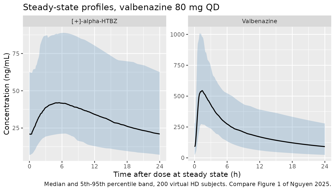
The parent profile peaks sharply within about 1.4 h of the dose and falls steeply, while the metabolite is nearly flat across the interval – the shape Figure 1 shows, and the reason the paper’s exposure metrics for the metabolite are so insensitive to which one is chosen.
Replicating Figure 2 – exposure overlap between the TD and HD cohorts
Figure 2 makes the paper’s central claim about generalising the TD dose to HD: the individual steady-state AUC distributions of both analytes overlap substantially between the two cohorts. Gate 2 already reproduced both cohorts’ published quantiles; here they are drawn together at 80 mg.
gate2 |>
  filter(dose == 80) |>
  mutate(quantile = recode(quantile, p5_auc = "5th", median = "Median",
                           p95_auc = "95th"),
         quantile = factor(quantile, levels = c("5th", "Median", "95th"))) |>
  ggplot(aes(x = cohort)) +
  geom_linerange(
    data = ~ tidyr::pivot_wider(.x, id_cols = cohort, names_from = quantile,
                                values_from = simulated),
    aes(ymin = `5th`, ymax = `95th`), linewidth = 6, colour = "grey80"
  ) +
  geom_point(aes(y = simulated, shape = quantile), size = 3) +
  geom_point(aes(y = published, colour = "Published (Table 2)"),
             shape = 4, size = 3, stroke = 1.2) +
  scale_colour_manual(values = c("Published (Table 2)" = "firebrick"), name = NULL) +
  labs(x = NULL, y = "[+]-alpha-HTBZ AUC24,ss (ng*h/mL)", shape = "Simulated",
       title = "Steady-state metabolite exposure at 80 mg QD, TD vs HD",
       caption = "Bars span the 5th-95th percentile. Compare Figure 2 of Nguyen 2025.")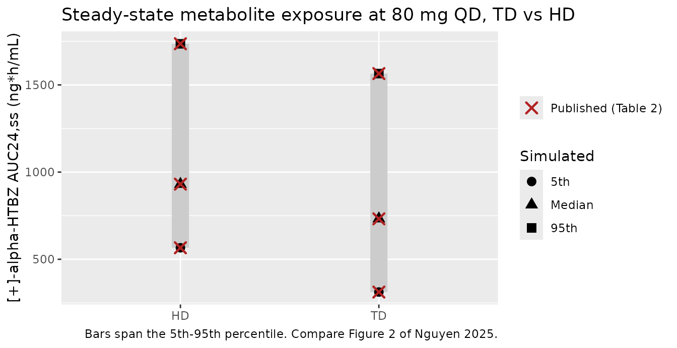
The two cohorts overlap across most of their range, with the HD distribution shifted modestly higher – consistent with the paper’s finding that HD subjects’ metabolite clearance is somewhat lower while “the range of individual exposure predictions remained consistent across populations”.
Exposure-efficacy model
Placebo time course
The placebo model rises with a 9.18-day onset half-life, is
multiplied by an attenuation factor from day TATT = 59
onward, and therefore peaks exactly at TATT. The paper’s
exploratory observation was that “the placebo effect appeared to
diminish after approximately 8 weeks” (day 56).
pbo_ev <- data.frame(
  id = 1L, time = seq(0, 98, by = 0.5), amt = NA_real_, evid = 0L,
  cmt = NA_character_, dvid = 1L, AUC_HTBZ = 0, PLACEBO = 1
)
pbo <- rxode2::rxSolve(tmc |> rxode2::zeroRe(), pbo_ev,
                       returnType = "data.frame")
#> ℹ omega/sigma items treated as zero: 'etapmax', 'etalec50'
stopifnot(all(is.finite(pbo$tmccfb)))

peak_day <- pbo$time[which.min(pbo$tmccfb)]
stopifnot(abs(peak_day - 59) < 1)

ggplot(pbo, aes(time, tmccfb)) +
  geom_hline(yintercept = 0, linetype = 3) +
  geom_vline(xintercept = 59, linetype = 2, colour = "firebrick") +
  geom_line(linewidth = 0.8) +
  annotate("text", x = 59, y = -0.3, label = "TATT = 59 d",
           hjust = -0.1, colour = "firebrick", size = 3.2) +
  labs(x = "Days since first dose", y = "Change from baseline in TMC score",
       title = "Typical-value placebo response",
       caption = "Asymptotic-exponential onset with attenuation from day 59. Compare Figure 3a of Nguyen 2025.")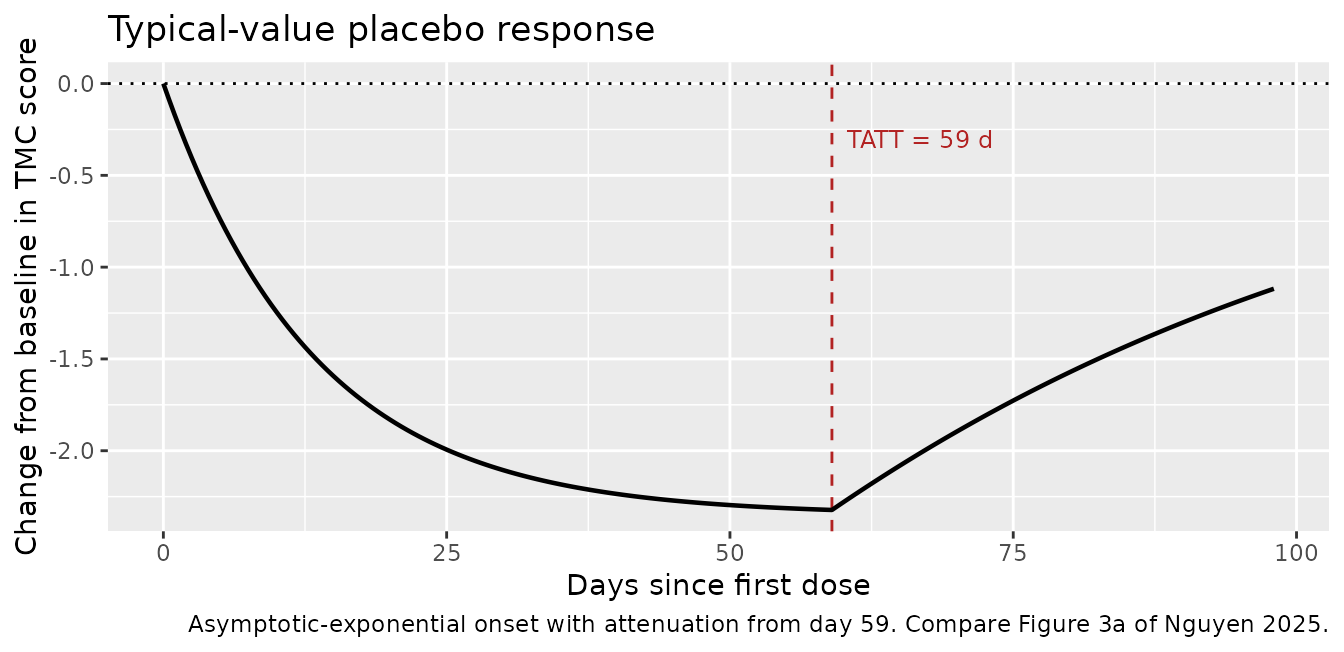
The typical-value placebo effect peaks at 59 days at -2.32 TMC points, and has decayed to -1.46 points by week 12 (day 84).
Gate 5 – Table 4 reproduced
Table 4 compares simulated mean TMC change from baseline at steady
state against the observed means. Reproducing it requires the
inter-individual variability to be active: with 125% CV on
EC50, subjects with a low EC50 saturate the
Emax term, so the arithmetic mean response is materially larger in
magnitude than the typical-value prediction – most of all at the lowest
exposures.
Two readings of Table 4’s window were tested. Its heading says “Weeks 10 and 12 of the Maintenance Period”, but the placebo value matches the model at week 12 alone (day 84), not the average of weeks 10 and 12; both are reported below.
set.seed(20250819)
n_er  <- 500L    # virtual subjects per replicate, as in the paper
n_rep <- 200L    # replicates (the paper used 1000; 200 is ample here)

# Per-dose AUC distribution: lognormal matched to the HD median and the
# 5th-95th spread of Table 2.
auc_dist <- auc_t2 |>
  filter(cohort == "HD") |>
  pivot_wider(names_from = quantile, values_from = published) |>
  mutate(sdlog = (log(p95_auc) - log(p5_auc)) / (2 * qnorm(0.95)))

sim_arm <- function(auc, placebo, day) {
  ev <- data.frame(
    id = seq_along(auc), time = day, amt = NA_real_, evid = 0L,
    cmt = NA_character_, dvid = 1L, AUC_HTBZ = auc, PLACEBO = placebo
  )
  rxode2::rxSolve(tmc, ev, returnType = "data.frame")$tmccfb
}

mean_response <- function(auc_fun, placebo, day) {
  mean(replicate(n_rep, mean(sim_arm(auc_fun(), placebo, day))))
}

gate5 <- bind_rows(
  tibble(arm = "Placebo", dose = 0,
         wk12 = mean_response(function() rep(0, n_er), 1, 84),
         wk10 = mean_response(function() rep(0, n_er), 1, 70)),
  bind_rows(lapply(seq_len(nrow(auc_dist)), function(i) {
    r <- auc_dist[i, ]
    draw <- function() rlnorm(n_er, log(r$median), r$sdlog)
    tibble(arm = paste0(r$dose, " mg"), dose = r$dose,
           wk12 = mean_response(draw, 0, 84),
           wk10 = mean_response(draw, 0, 70))
  }))
) |>
  mutate(
    wk10_12   = (wk10 + wk12) / 2,
    published = c(-1.46, -1.77, -3.17, -4.37, -5.27),
    pct_wk12  = 100 * (wk12 - published) / abs(published)
  )

stopifnot(max(abs(gate5$pct_wk12)) < 5)

gate5 |>
  select(arm, wk12, wk10_12, published, pct_wk12) |>
  rename(
    "Arm"                            = arm,
    "Simulated, week 12"             = wk12,
    "Simulated, mean of weeks 10+12" = wk10_12,
    "Table 4 simulated mean"         = published,
    "Week-12 difference (%)"         = pct_wk12
  ) |>
  knitr::kable(digits = c(0, 2, 2, 2, 1),
caption = "Gate 5: mean TMC change from baseline versus Nguyen 2025 Table 4. The week-12 column matches; the weeks-10-and-12 average does not.")| Arm | Simulated, week 12 | Simulated, mean of weeks 10+12 | Table 4 simulated mean | Week-12 difference (%) |
|---|---|---|---|---|
| Placebo | -1.46 | -1.68 | -1.46 | 0.3 |
| 20 mg | -1.74 | -1.74 | -1.77 | 1.7 |
| 40 mg | -3.16 | -3.16 | -3.17 | 0.4 |
| 60 mg | -4.28 | -4.29 | -4.37 | 1.9 |
| 80 mg | -5.22 | -5.22 | -5.27 | 0.9 |
Every arm agrees with Table 4 to within 1.9% on the week-12 reading, against 14.8% for the weeks-10-and-12 average. The week-12 interpretation is therefore the one that reproduces the paper, and is what this vignette uses.
Replicating Figure 4 – the exposure-response curve
Figure 4 plots the predicted change from baseline in TMC score
against [+]-alpha-HTBZ exposure over 0-3000 ng*h/mL, with
the observed dose-group exposure distributions marked underneath.
set.seed(20250819)
auc_grid <- seq(0, 3000, by = 60)
n_grid <- 200L

er_curve <- bind_rows(lapply(seq_along(auc_grid), function(i) {
  a <- auc_grid[i]
  ev <- data.frame(
    id = (i - 1L) * n_grid + seq_len(n_grid), time = 84, amt = NA_real_,
    evid = 0L, cmt = NA_character_, dvid = 1L, AUC_HTBZ = a, PLACEBO = 0
  )
  y <- rxode2::rxSolve(tmc, ev, returnType = "data.frame")$tmccfb
  tibble(auc = a, Q05 = quantile(y, 0.05), Q50 = median(y),
         Q95 = quantile(y, 0.95), mean = mean(y))
}))
stopifnot(nrow(er_curve) == length(auc_grid), all(is.finite(er_curve$Q50)))

dose_boxes <- auc_dist |>
  transmute(dose = factor(dose), lo = p5_auc, mid = median, hi = p95_auc)

ggplot(er_curve, aes(auc)) +
  geom_ribbon(aes(ymin = Q05, ymax = Q95), alpha = 0.2, fill = "darkolivegreen") +
  geom_line(aes(y = Q50), linewidth = 0.8) +
  geom_hline(yintercept = -4.0, linetype = 2, colour = "firebrick") +
  annotate("text", x = 2950, y = -4.0, label = "MCID -4.0", vjust = -0.5,
           hjust = 1, colour = "firebrick", size = 3.2) +
  geom_linerange(data = dose_boxes, inherit.aes = FALSE,
                 aes(y = 1.5, xmin = lo, xmax = hi, colour = dose),
                 linewidth = 2.5) +
  geom_point(data = dose_boxes, inherit.aes = FALSE,
             aes(x = mid, y = 1.5, colour = dose), size = 2.5) +
  labs(x = "[+]-alpha-HTBZ AUC24,ss (ng*h/mL)",
       y = "Change from baseline in TMC score",
       colour = "Dose (mg QD)",
       title = "Predicted exposure-response for chorea",
       caption = paste("Median and 5th-95th percentile band, 200 virtual subjects per exposure.",
                       "Bars show the Table 2 HD exposure ranges. Compare Figure 4 of Nguyen 2025."))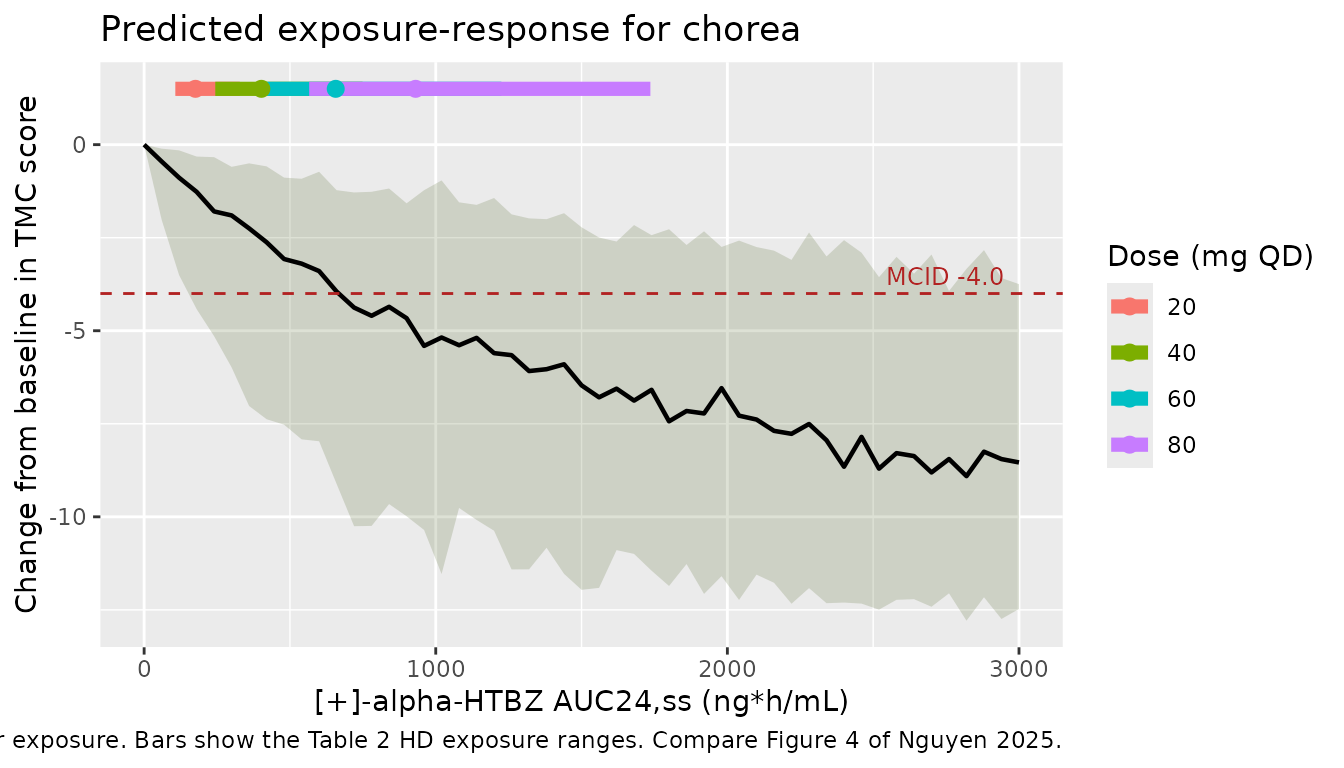
The dashed line marks the minimal clinically important difference of -4.0 TMC points (CGI-S anchor; Nguyen 2025 Discussion). The median predicted response crosses it at about 680 ng*h/mL, which sits inside the exposure range of the 60 mg and 80 mg dose groups and outside that of 20 mg – the quantitative basis for the paper’s recommendation of 40 to 80 mg once daily with 80 mg as the target.
Note the paper’s own caveat, which this figure inherits: most observed data lay at or below 1500 ngh/mL, so the plateau above roughly 2000 ngh/mL is carried by the Emax asymptote rather than by data.
Assumptions and deviations
Non-paper-derived values
-
Molecular weights.
MW(valbenazine) = 418.57 g/molandMW([+]-alpha-HTBZ) = 319.44 g/molare standard chemical constants (PubChem CIDs 24756910 and 92987) and are not reported in Nguyen 2025. They are required because the paper fitted natural-log-transformed molar concentrations (soFM = 0.207is a molar fraction) while its exposure summaries, assay LLOQs and the E-REC50are all in mass units. The conversion enters the model exactly once, in the metabolite-formation flux. Gate 1 and Gate 2 confirm the resulting exposures reproduce Table 2 to within 0.1%, which would not hold if either weight were materially wrong. Doses are taken as valbenazine free-base equivalents, matching the marketed capsule labelling.
Interpretation choices
-
EC50encoding.lec50 = 7.50is the THETA printed in Table 3;exp(7.50) = 1808ng*h/mL against the 1820 printed as the back-transformed estimate (1820 corresponds tolog(EC50) = 7.5066, so the printed THETA is rounded). The reported CI back-transforms exactly. The reported THETA is encoded, makingEC500.7% lower than the printed value. - Table 4 evaluation time. Table 4’s heading says “Weeks 10 and 12 of the Maintenance Period”, but its numbers match the model evaluated at week 12 alone; the average of weeks 10 and 12 over-predicts the placebo arm by 15%. Gate 5 reports both and uses week 12.
-
Placebo attenuation as a clamp. The printed placebo
equation is a two-case piecewise function in
trelative toTATT. It is encoded asexp(-katt * max(time - tswitch, 0)), which is algebraically identical and avoids a branch insidemodel(). -
0.693versuslog(2). The rate constants use the paper’s literalKPBO = 0.693 / HLPLBrather thanlog(2) / HLPLB, reproducing the printed definition; the difference is 0.02%. -
Transit chain length. “A total of four transit
absorption compartments were identified” is read literally as four
transit compartments between the depot and the central compartment, all
transferring at
KTR = KA. The steady-state AUC is invariant to this reading (mass balance), and the metaboliteCmaxreproduces Table 2 to within 2.2%. -
(DOSE - 1 mg)offset. Supplemental Table S2 equation (4) offsets the dose by the 1 mg anchor. Gate 4 confirms this against the Discussion’s 1.09-/1.16-fold statement; the offset is small enough that a bareDOSEform would also pass that check, so Table S2 is the authority. The model clamps the offset at zero so a sub-1-mg dose cannot driveF1below the anchor. - Diagonal OMEGA. Table 1 reports four IIV variances with no covariances, so the omega matrix is encoded as diagonal.
Cohort assumptions for the simulations
- Body weight. KINECT-HD reports median 75.8 kg over 41.0-134 kg (Supplemental Table S6) but no distributional form; a lognormal matched on the median and truncated to the observed range is used, and the parent exposure is only weakly weight-dependent (the paper reports under 30% variation across the observed range).
- CYP2D6 phenotype. Frequencies are the KINECT-HD Table S5 values renormalised over the 97.6% of subjects with a genotype result; the 2.4% with missing genotype are assigned proportionally rather than to a single category. Per Table 1 footnote a, subjects reported as either intermediate or extensive were counted as intermediate.
-
Fed and formulation state. Both phase 3 studies
used capsules (
FORM_SOLUTION = 0) and KINECT-HD dosed “without regard to food” (Supplemental Table S1). The fasted reference (FED = 0) is used throughout, which is the state the Table 1 typical values correspond to. -
Sampling design.
SAMPLE_INTENSIVE = 1is used in the simulations. It affects only the residual-error magnitude, so it does not enter any of the gates above, all of which compare model predictions rather than simulated observations. -
Individual EBEs versus typical values. Table 2
summarises Bayesian post-hoc estimates within a cohort, not
typical-value predictions. Gate 2 and the PKNCA section substitute the
cohort’s own published
CLMquantile from Supplemental Table S3; this is a published input, not a fitted adjustment, and no model parameter was tuned anywhere in this vignette.
Errata found in the source
-
Table 2
Cavgcolumn. The reportedCavgexceeds the reportedCmaxin all eight rows of Table 2, which is impossible, and sits a constant 1.31x aboveAUC24 / 24– implying an interval of about 18.3 h rather than 24 h.AUC24,CmaxandCminfrom the same table are all reproduced by the model, so this is a defect in the publishedCavgderivation. See the “Cavg” section above. No value in either model file depends on this column. -
Unicode minus signs. Table 1 of the PDF uses U+2212
rather than an ASCII hyphen for negative estimates, which defeats naive
text extraction. The four negative coefficients (
-0.685,-0.0646,-0.516,-0.281) were verified directly against the rendered table.
New canonical register entries
This extraction added four entries, each a member of an existing canonical family (see the pull-request description for the rationale):
-
htbz– metabolite suffix for[+]-alpha-dihydrotetrabenazine (inst/references/compartment-names.md; direct analogue ofbibf). -
tmccfb– UHDRS Total Maximal Chorea change-from-baseline PD output compartment (inst/references/compartment-names.md; follows thecfbsuffix convention ofdruglikingvascfb). -
CYP2D6_IM– CYP2D6 intermediate-metabolizer indicator (inst/references/covariate-columns.md). Required rather than optional here: this paper pools ultra-rapid with extensive as the reference, so the existingCYP2D6_EMcannot be inverted to express it without wrongly applying the intermediate-metabolizer reduction to ultra-rapid metabolizers. -
AUC_HTBZ– daily steady-state metabolite AUC exposure driver (inst/references/covariate-columns.md; member of theAUC_<DRUG>family).