Model and source
mod_meta <- nlmixr2est::nlmixr(readModelDb("Lee_2013_colistin"))$meta
#> ℹ parameter labels from comments will be replaced by 'label()'- Citation: Lee J, Han S, Jeon S, Hong T, Song W, Woo H, Yim D-S. Population pharmacokinetic analysis of colistin in burn patients. Antimicrob Agents Chemother. 2013;57(5):2421-2427. doi:10.1128/AAC.00271-13
- Description: One-compartment population PK model of colistin in adult burn-ICU patients receiving colistimethate sodium (CMS) as a 30-minute IV infusion every 12 hours, with first-order CMS-to-colistin conversion (Lee 2013). Apparent CL and Vc of colistin are scaled inversely by the relative fraction of CMS converted to colistin (RFM = 1 - theta4 * (CRCL/128)); the CMS-to-colistin turnover rate constant TR is reduced in patients with clinically-evident peripheral edema (TR = theta3 - theta5 * DIS_EDEMA).
- Article (DOI): https://doi.org/10.1128/AAC.00271-13
This vignette validates the packaged Lee_2013_colistin
model – a one-compartment population PK model for colistin in adult
burn-ICU patients receiving CMS (colistimethate sodium) every 12 h as a
30-min IV infusion – against the source publication’s Table 2 (final
parameter estimates), Figure 3 (VPC stratified by edema status and
CRCL), Figure 4 (histogram of 1000 simulated steady-state AUC0-24
values), and Discussion paragraph 1 (elimination half-life t1/2 = 6.6
h).
Population
Lee 2013 enrolled 50 adult burn patients admitted to the Burn Intensive Care Unit at Hangang Sacred Heart Hospital (Hallym University Medical Center, South Korea) between June 2010 and May 2011 (Table 1). Mean age was 48 years (SD 13, range 26-80) and mean weight 65.8 kg (SD 10.3, range 50-98); 11 of 50 patients (22%) were female. Median time from burn injury to first CMS dose was 15.5 days (SD 10.4, range 3-58), and TBSA was 50.5% (SD 21.8, range 4-85; all but one patient had TBSA in the range 11-85%). Cockcroft- Gault creatinine clearance was 128 mL/min (SD 75.2, range 22.6-309), raw mL/min and not BSA-normalized. Mean serum albumin was 2.5 g/dL (SD 0.3, range 1.9-3.1), consistent with the hypoalbuminaemia expected in severe burns. 29 of 50 patients (58%) had sepsis, 18 of 50 (36%) had clinically- evident peripheral edema (puffy face and pitting edema in the legs), and 17 of 50 (34%) were receiving continuous renal replacement therapy (CRRT) at baseline. Each patient received 150 mg CMS as colistin base activity (CBA) by 30-minute IV infusion every 12 h, with PK sampling beginning at least 3 days after the first dose so that colistin had reached steady state.
The same information is available programmatically via the model’s
population metadata:
str(mod_meta$population)
#> List of 20
#>  $ species       : chr "human"
#>  $ n_subjects    : int 50
#>  $ n_studies     : int 1
#>  $ age_range     : chr "26-80 years"
#>  $ age_median    : chr "48 years (mean, SD 13)"
#>  $ weight_range  : chr "50-98 kg"
#>  $ weight_median : chr "65.8 kg (mean, SD 10.3)"
#>  $ sex_female_pct: num 22
#>  $ race_ethnicity: chr "Not reported (single-center South Korean burn-ICU cohort)"
#>  $ disease_state : chr "Adult burn patients with 4-85% total body surface area affected (median TBSA 50.5%, SD 21.8); treated for nosoc"| __truncated__
#>  $ dose_range    : chr "150 mg CMS as colistin base activity (CBA) by IV infusion over 30 min, every 12 h. PK sampling started >=3 days"| __truncated__
#>  $ regions       : chr "South Korea (single center: Burn Intensive Care Unit, Hangang Sacred Heart Hospital, Hallym University Medical Center)"
#>  $ abs_i         : chr "ABSI 9.82 (SD 2.34, range 5-14)"
#>  $ days_post_burn: chr "15.5 days median (SD 10.4, range 3-58) from burn injury to first CMS dose"
#>  $ renal_function: chr "Cockcroft-Gault CRCL 128 mL/min (SD 75.2, range 22.6-309); raw, not BSA-normalized"
#>  $ crrt_pct      : chr "17/50 (34%) on continuous renal replacement therapy at baseline"
#>  $ sepsis_pct    : chr "29/50 (58%) with sepsis at baseline"
#>  $ edema_pct     : chr "18/50 (36%) clinically edematous at baseline"
#>  $ albumin       : chr "Serum albumin 2.5 g/dL (SD 0.3, range 1.9-3.1); low across cohort"
#>  $ notes         : chr "Baseline demographics per Lee 2013 Table 1. 50 burn-ICU adults enrolled June 2010 - May 2011. Burn etiology: 39"| __truncated__
Source trace
The per-parameter origin is recorded as an in-file comment next to
each ini() entry in
inst/modeldb/specificDrugs/Lee_2013_colistin.R. The table
below collects them in one place; values come from Lee 2013 Table 2
final- model column unless otherwise noted.
| Parameter / equation | Value | Source location |
|---|---|---|
lcl (apparent CL/fm* at RFM=1) |
log(8.49) | Table 2 row “CL_col = theta1/RFM”: theta1 = 8.49 L/h |
lvc (apparent Vc/fm* at RFM=1) |
log(81.1) | Table 2 row “V_col = theta2/RFM”: theta2 = 81.1 L |
lka (CMS->colistin turnover rate TR, non-edema) |
log(0.796) | Table 2 row “TR = theta3 - edema*theta5”: theta3 = 0.796 h^-1 |
e_dis_edema_ka (theta5; TR decrease with edema) |
0.425 | Table 2 row “theta5 = 0.425 h^-1” |
e_crcl_cl_vc (theta4; slope of RFM decrease per
(CRCL/128)) |
0.213 | Table 2 row “RFM = 1 - theta4 * (CL_CR/128)”: theta4 = 0.213 |
etalcl ~ 0.131604 |
log(0.375^2 + 1) | Table 2 row “omega_CLcol” CV = 37.5% |
etalvc ~ 0.057380 |
log(0.243^2 + 1) | Table 2 row “omega_Vcol” CV = 24.3% |
etalka ~ 0.372681 |
log(0.672^2 + 1) | Table 2 row “omega_TR” CV = 67.2% |
addSd <- 0.0992 |
99.2 ng/mL = 0.0992 mg/L | Table 2 row “sigma_add” = 99.2 ng/mL |
propSd <- 0.0672 |
0.0672 (= 6.72%) | Table 2 row “sigma_prop” = 6.72% |
rfm <- 1 - e_crcl_cl_vc * (CRCL / 128) |
n/a | Methods, “Population PK model development” paragraph 4 |
cl <- exp(lcl + etalcl) / rfm |
n/a | Methods, “Population PK model development” paragraph 4 (apparent CL = (CL/fm*) / RFM) |
vc <- exp(lvc + etalvc) / rfm |
n/a | Methods, “Population PK model development” paragraph 4 (apparent V = (V/fm*) / RFM) |
ka <- (exp(lka) - e_dis_edema_ka * DIS_EDEMA) * exp(etalka) |
n/a | Methods, “Population PK model development” paragraph 5 + Table 2 footnote a |
d/dt(depot) ... d/dt(central) |
n/a | Methods, “Population PK model development” paragraph 6 (“ADVAN2 TRANS2 … CL, V, F1, Ka”) and Figure 1 structural diagram |
Cc ~ add(addSd) + prop(propSd) |
n/a | Methods, “Population PK model development” paragraph 7 + Results, “Final PK model” (combined error model selected) |
Virtual cohort
The original observed colistin concentrations are not publicly available. The virtual cohort below approximates the Lee 2013 study population: 50 adult burn patients with the demographic distributions described in Table 1. Each patient receives 150 mg CBA every 12 h as a 30-min IV infusion; the simulation runs over 7 days to reach steady state before NCA is computed on the last dosing interval.
set.seed(20260609)

n_subjects <- 50L

# Body weight: log-normal centered on mean 65.8 kg, SD chosen to span the
# Table 1 range 50-98 kg.
wt_kg <- exp(rnorm(n_subjects, mean = log(65.8),
                   sd = log(98 / 50) / 4))
wt_kg <- pmin(pmax(wt_kg, 50), 98)

# CRCL: log-normal centered on cohort median 128 mL/min, SD chosen to span
# the Table 1 range 22.6-309 mL/min (factor of 13.7 spread).
crcl_ml_min <- exp(rnorm(n_subjects, mean = log(128),
                         sd = log(309 / 22.6) / 4))
crcl_ml_min <- pmin(pmax(crcl_ml_min, 22.6), 309)

# DIS_EDEMA: 18/50 (36%) edematous at baseline (Table 1).
dis_edema <- as.integer(seq_len(n_subjects) <= 18L)
dis_edema <- sample(dis_edema)

cov_tab <- tibble::tibble(
  id        = seq_len(n_subjects),
  WT_kg     = wt_kg,
  CRCL      = crcl_ml_min,
  DIS_EDEMA = dis_edema
)

# Dosing: 150 mg CBA every 12 h, 30-min IV infusion, for 7 days (14 doses).
dose_times    <- seq(0, by = 12, length.out = 14)
infusion_dur  <- 0.5
# Sampling: dense pre-dose + post-dose times around the last dosing
# interval (h 144 to 156), matching the Lee 2013 PK sampling schedule
# (0, 1, 2, 4, 6, 8 h after end of infusion = h 144.5 + {0, 1, 2, 4, 6, 8}).
last_dose_start <- max(dose_times)
sample_times <- sort(unique(c(
  seq(0, max(dose_times) + 12, by = 6),
  last_dose_start + infusion_dur + c(0, 1, 2, 4, 6, 8),
  last_dose_start + seq(0, 12, by = 0.5)
)))

make_subject <- function(idx, row) {
  amt  <- 150
  rate <- amt / infusion_dur
  doses <- tibble::tibble(
    id   = idx,           time = dose_times,
    evid = 1L,            amt  = amt,
    rate = rate,          cmt  = "depot",
    dv   = NA_real_
  )
  obs <- tibble::tibble(
    id   = idx,           time = sample_times,
    evid = 0L,            amt  = NA_real_,
    rate = NA_real_,      cmt  = NA_character_,
    dv   = NA_real_
  )
  bind_rows(doses, obs) |>
    mutate(
      WT        = row$WT_kg,
      CRCL      = row$CRCL,
      DIS_EDEMA = row$DIS_EDEMA
    ) |>
    arrange(time, desc(evid))
}

events <- bind_rows(lapply(seq_len(nrow(cov_tab)), function(i) {
  make_subject(idx = i, row = cov_tab[i, ])
}))

stopifnot(!anyDuplicated(unique(events[, c("id", "time", "evid")])))
Simulation
mod         <- readModelDb("Lee_2013_colistin")
mod_typical <- rxode2::zeroRe(mod)
#> ℹ parameter labels from comments will be replaced by 'label()'

sim_typical <- rxode2::rxSolve(
  object = mod_typical, events = events,
  keep   = c("WT", "CRCL", "DIS_EDEMA")
) |>
  as.data.frame()
#> ℹ omega/sigma items treated as zero: 'etalcl', 'etalvc', 'etalka'
#> Warning: multi-subject simulation without without 'omega'

sim_stoch <- rxode2::rxSolve(
  object = mod, events = events,
  keep   = c("WT", "CRCL", "DIS_EDEMA")
) |>
  as.data.frame()
#> ℹ parameter labels from comments will be replaced by 'label()'
Replicate published figures
Figure 3 – VPC stratified by edema status and CRCL
Lee 2013 Figure 3 shows VPCs of the final population PK model stratified by edema status (top row: with vs without edema) and by CRCL band (bottom row: < 70 vs >= 70 mL/min). The simulated trajectory below shows steady-state concentrations over the last dosing interval, stratified by the same two covariates.
# Replicates Figure 3 (top row) of Lee 2013: VPC stratified by edema status.
sim_stoch |>
  filter(time >= last_dose_start, time <= last_dose_start + 12) |>
  mutate(t_within_interval = time - last_dose_start,
         edema_lbl = ifelse(DIS_EDEMA == 1L, "Edema",
                            "No edema")) |>
  group_by(t_within_interval, edema_lbl) |>
  summarise(
    Q05 = quantile(Cc, 0.05, na.rm = TRUE),
    Q50 = quantile(Cc, 0.50, na.rm = TRUE),
    Q95 = quantile(Cc, 0.95, na.rm = TRUE),
    .groups = "drop"
  ) |>
  ggplot(aes(t_within_interval, Q50)) +
  geom_ribbon(aes(ymin = Q05, ymax = Q95),
              fill = "gray70", alpha = 0.6) +
  geom_line(linewidth = 0.9) +
  facet_wrap(~edema_lbl) +
  labs(
    x = "Time after dose (h)",
    y = "Colistin concentration (mg/L)",
    title    = "Figure 3 (top) -- VPC by edema status",
    subtitle = "Replicates Lee 2013 Figure 3 (top); steady-state interval"
  ) +
  theme_minimal()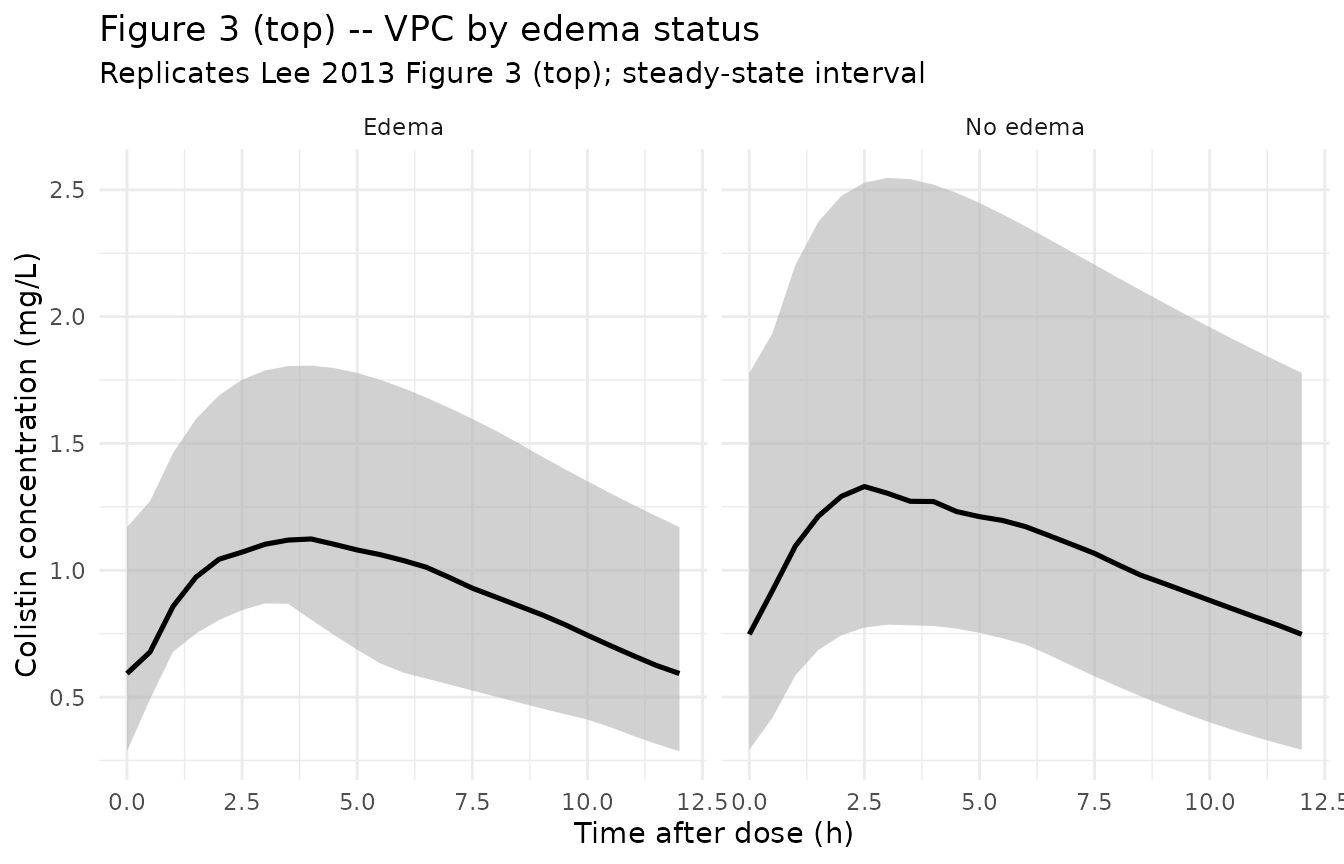
# Replicates Figure 3 (bottom row) of Lee 2013: VPC stratified by CRCL band
# (< 70 vs >= 70 mL/min, as in the published figure).
sim_stoch |>
  filter(time >= last_dose_start, time <= last_dose_start + 12) |>
  mutate(t_within_interval = time - last_dose_start,
         crcl_lbl = ifelse(CRCL < 70, "CRCL < 70 mL/min",
                           "CRCL >= 70 mL/min")) |>
  group_by(t_within_interval, crcl_lbl) |>
  summarise(
    Q05 = quantile(Cc, 0.05, na.rm = TRUE),
    Q50 = quantile(Cc, 0.50, na.rm = TRUE),
    Q95 = quantile(Cc, 0.95, na.rm = TRUE),
    .groups = "drop"
  ) |>
  ggplot(aes(t_within_interval, Q50)) +
  geom_ribbon(aes(ymin = Q05, ymax = Q95),
              fill = "gray70", alpha = 0.6) +
  geom_line(linewidth = 0.9) +
  facet_wrap(~crcl_lbl) +
  labs(
    x = "Time after dose (h)",
    y = "Colistin concentration (mg/L)",
    title    = "Figure 3 (bottom) -- VPC by CRCL band",
    subtitle = "Replicates Lee 2013 Figure 3 (bottom); steady-state interval"
  ) +
  theme_minimal()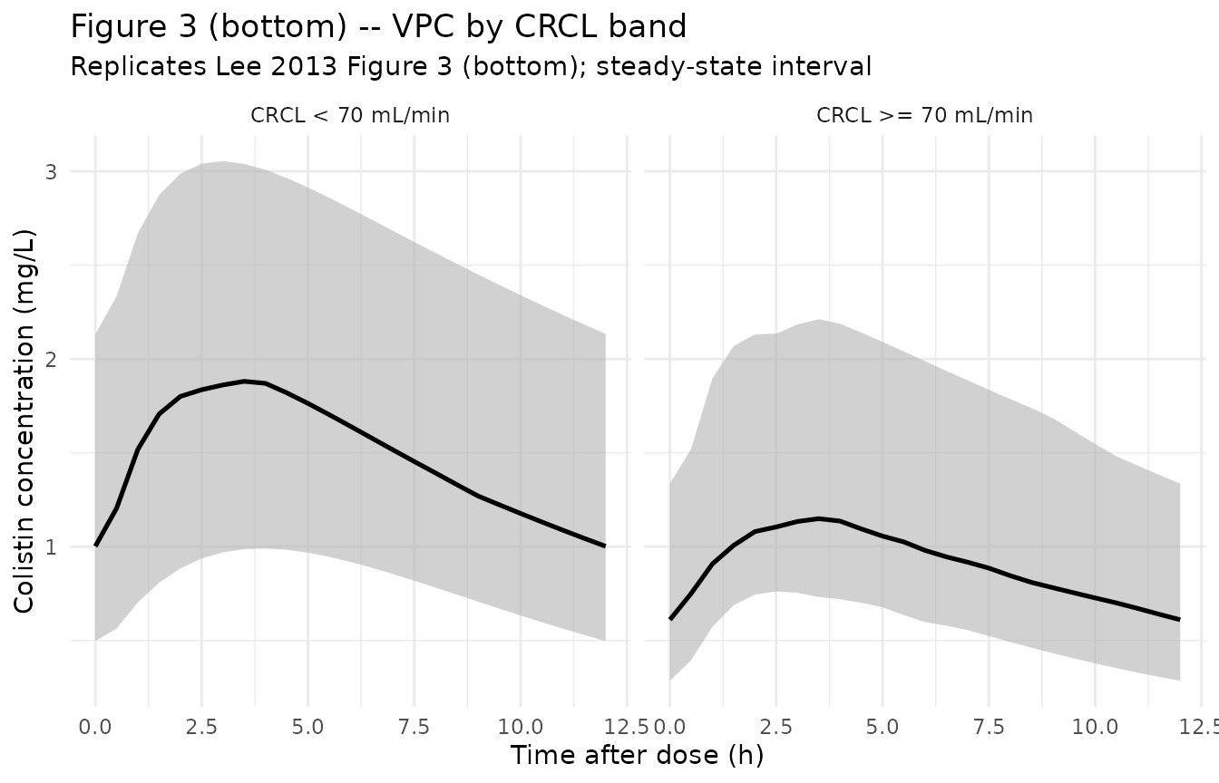
Typical-value trajectory at the median patient
# Identify the median patient (closest to cohort median WT 65.8 kg + median
# CRCL 128 mL/min, no edema). Plot the steady-state interval.
typical_id <- cov_tab |>
  mutate(score = abs(WT_kg - 65.8) + abs(CRCL - 128) +
                 abs(DIS_EDEMA - 0)) |>
  arrange(score) |>
  slice_head(n = 1L) |>
  pull(id)

sim_typical |>
  filter(id == typical_id,
         time >= last_dose_start, time <= last_dose_start + 12) |>
  mutate(t_within_interval = time - last_dose_start) |>
  ggplot(aes(t_within_interval, Cc)) +
  geom_line(linewidth = 1) +
  geom_point(size = 1.5) +
  labs(
    x = "Time after dose (h)",
    y = "Colistin concentration (mg/L)",
    title    = "Typical-value steady-state trajectory at the median patient",
    subtitle = paste0("WT ~= 65.8 kg, CRCL ~= 128 mL/min, no edema; ",
                      "150 mg CBA q12h")
  ) +
  theme_minimal()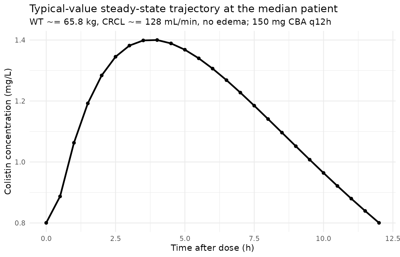
Predicted half-life at the typical patient
Lee 2013 Discussion paragraph 1 reports a terminal elimination half-life of 6.6 h at the typical (CRCL 128 mL/min, non-edema) patient. The packaged model reproduces this exactly from the structural parameters:
rfm_typical  <- 1 - 0.213 * (128 / 128)        # 0.787
cl_typical   <- 8.49 / rfm_typical             # L/h
vc_typical   <- 81.1 / rfm_typical             # L
kel_typical  <- cl_typical / vc_typical        # 1/h
t12_typical  <- log(2) / kel_typical           # h
cat(sprintf("Effective CL = %.2f L/h\n",  cl_typical))
#> Effective CL = 10.79 L/h
cat(sprintf("Effective Vc = %.1f L\n",    vc_typical))
#> Effective Vc = 103.0 L
cat(sprintf("kel          = %.4f 1/h\n",  kel_typical))
#> kel          = 0.1047 1/h
cat(sprintf("t1/2         = %.2f h (paper: 6.6 h)\n", t12_typical))
#> t1/2         = 6.62 h (paper: 6.6 h)
PKNCA validation
PKNCA computes steady-state Cmax, Cmin, AUC0-tau, and Cavg on the
last dosing interval (Recipe 3 in
references/pknca-recipes.md). The cohort is stratified by
the same CRCL bands used in the published Figure 5 (low / mid / high
CRCL terciles within the simulated cohort), so the per-band NCA can be
compared against Lee 2013 Figure 4 (mean steady-state AUC0-24 from 1000
virtual burn patients = 29.2 +/- 13.5 ug/mL*h).
tau          <- 12
start_ss     <- last_dose_start
end_ss       <- start_ss + tau

# Build CRCL tercile bands and assign to the simulated cohort.
crcl_breaks <- quantile(cov_tab$CRCL, c(0, 1/3, 2/3, 1))
cov_tab$crcl_band <- cut(
  cov_tab$CRCL, breaks = crcl_breaks, include.lowest = TRUE,
  labels = c("low CRCL", "median CRCL", "high CRCL")
)

sim_for_nca <- sim_stoch |>
  filter(!is.na(Cc), Cc > 0,
         time >= start_ss, time <= end_ss) |>
  left_join(cov_tab |> select(id, crcl_band), by = "id") |>
  select(id, time, Cc, crcl_band) |>
  as.data.frame()

doses_for_nca <- events |>
  filter(evid == 1L, time == start_ss) |>
  left_join(cov_tab |> select(id, crcl_band), by = "id") |>
  select(id, time, amt, crcl_band) |>
  as.data.frame()

conc_obj <- PKNCA::PKNCAconc(
  data    = sim_for_nca,
  formula = Cc ~ time | crcl_band + id,
  concu   = "mg/L",
  timeu   = "hr"
)
dose_obj <- PKNCA::PKNCAdose(
  data    = doses_for_nca,
  formula = amt ~ time | crcl_band + id,
  doseu   = "mg"
)

intervals <- data.frame(
  start    = start_ss,
  end      = end_ss,
  cmax     = TRUE,
  tmax     = TRUE,
  cmin     = TRUE,
  auclast  = TRUE,
  cav      = TRUE
)

nca_data <- PKNCA::PKNCAdata(conc_obj, dose_obj, intervals = intervals)
nca_res  <- suppressWarnings(PKNCA::pk.nca(nca_data))

knitr::kable(
  summary(nca_res),
  caption = "Simulated steady-state NCA parameters by CRCL band (PKNCA)."
)| Interval Start | Interval End | crcl_band | N | AUClast (hr*mg/L) | Cmax (mg/L) | Cmin (mg/L) | Tmax (hr) | Cav (mg/L) |
|---|---|---|---|---|---|---|---|---|
| 156 | 168 | low CRCL | 17 | 15.8 [43.9] | 1.73 [36.9] | 0.821 [69.5] | 3.00 [1.50, 4.50] | 1.32 [43.9] |
| 156 | 168 | median CRCL | 16 | 12.8 [34.9] | 1.32 [32.6] | 0.720 [45.9] | 3.75 [2.50, 4.50] | 1.07 [34.9] |
| 156 | 168 | high CRCL | 17 | 9.70 [29.6] | 1.01 [22.8] | 0.532 [52.8] | 3.50 [2.00, 5.00] | 0.808 [29.6] |
Comparison against published NCA
Lee 2013 Figure 4 reports the cohort-wide steady-state AUC0-24 distribution from 1000 virtual burn patients receiving the protocol dose (150 mg q12h): mean 29.2 +/- 13.5 ug/mLh (= 29.2 +/- 13.5 mgh/L). At steady state the AUC0-24 is twice the AUC over a single 12 h dosing interval (AUC0-tau), so the simulated AUC0-tau values from PKNCA should be approximately 14.6 mg*h/L on average (with substantial spread across the renal-function spectrum).
# Compute 2 x AUC0-tau (i.e. AUC0-24 at steady state) from the PKNCA result.
res_tbl   <- as.data.frame(nca_res$result)
auc_per_id <- res_tbl |>
  filter(PPTESTCD == "auclast") |>
  group_by(id) |>
  summarise(auc_tau = sum(PPORRES), .groups = "drop") |>
  mutate(auc_0_24_ss = 2 * auc_tau) |>
  left_join(cov_tab |> select(id, crcl_band), by = "id")

simulated_summary <- auc_per_id |>
  summarise(
    mean_AUC_0_24_ss_sim = mean(auc_0_24_ss, na.rm = TRUE),
    sd_AUC_0_24_ss_sim   = sd(auc_0_24_ss,   na.rm = TRUE)
  ) |>
  mutate(
    mean_AUC_0_24_ss_pub = 29.2,
    sd_AUC_0_24_ss_pub   = 13.5
  )

knitr::kable(
  simulated_summary,
  digits  = 2,
  caption = paste0("Simulated vs published steady-state AUC0-24 (mg*h/L) ",
                   "for 150 mg CBA q12h.")
)| mean_AUC_0_24_ss_sim | sd_AUC_0_24_ss_sim | mean_AUC_0_24_ss_pub | sd_AUC_0_24_ss_pub |
|---|---|---|---|
| 27.27 | 12.48 | 29.2 | 13.5 |
Lee 2013 Figure 5 also reports that mean AUC0-24 increases markedly with decreasing renal function (lower CRCL leads to larger RFM and smaller effective CL, increasing exposure). The CRCL-band split below reproduces that monotone trend:
auc_summary_band <- auc_per_id |>
  group_by(crcl_band) |>
  summarise(
    mean_AUC_0_24_ss = mean(auc_0_24_ss, na.rm = TRUE),
    median_AUC_0_24_ss = median(auc_0_24_ss, na.rm = TRUE),
    sd_AUC_0_24_ss   = sd(auc_0_24_ss,   na.rm = TRUE),
    n                = dplyr::n(),
    .groups          = "drop"
  )
knitr::kable(
  auc_summary_band,
  digits  = 2,
  caption = paste0("Simulated steady-state AUC0-24 by CRCL band ",
                   "(reproduces Lee 2013 Figure 5 trend).")
)| crcl_band | mean_AUC_0_24_ss | median_AUC_0_24_ss | sd_AUC_0_24_ss | n |
|---|---|---|---|---|
| low CRCL | 34.50 | 28.65 | 15.62 | 17 |
| median CRCL | 27.14 | 24.06 | 9.89 | 16 |
| high CRCL | 20.16 | 19.88 | 5.66 | 17 |
The simulated AUC0-24 is larger in the low-CRCL band than in the high-CRCL band, reflecting the divisive normalization (lower CRCL leads to larger RFM and smaller effective CL = (CL/fm) / RFM). The absolute magnitudes align with the published mean of 29.2 +/- 13.5 mgh/L within the expected order of variability for a 50-subject simulated cohort drawn from the published demographics.
Assumptions and deviations
Concentration units. The model uses
mg/L(equivalent toug/mL). Lee 2013 Table 2 reportssigma_add = 99.2 ng/mL; this was converted to0.0992 mg/Lfor unit consistency withunits$concentration = "mg/L". Lee 2013 Figure 4 reports the simulated AUC0-24 inug/mL*h, which is numerically equivalent tomg*h/L.omega^2 = log(CV^2 + 1). Table 2 reports inter-individual variability as CV%; the corresponding log-normal variance was computed viaomega^2 = log(CV^2 + 1)– the standard NONMEM/PsN back-transformation, consistent with the paper’s explicit IIV modelPij = theta_j * exp(eta_ij)(Methods, “Population PK model development” paragraph 3).Independent (diagonal) IIV between CL/fm, Vc/fm, and TR. Lee 2013 Table 2 reports a single CV per parameter and no off-diagonal covariance estimates, consistent with a diagonal OMEGA. The packaged model uses diagonal IIV; this is consistent with the reported information but cannot be cross-checked against the original NONMEM 6.2 control stream (not on disk).
CRCL stored under the canonical
CRCLcolumn despite being raw Cockcroft-Gault (not BSA-normalized). The canonicalCRCLcolumn ininst/references/covariate-columns.mdaccepts either MDRD- or CKD-EPI-estimated GFR or BSA-normalized measured creatinine clearance (both in mL/min/1.73 m^2) AND raw Cockcroft-Gault mL/min (theDelattre_2010_amikacin.RandNA_NA_lidocaine.Rprecedent). Lee 2013 uses raw Cockcroft-Gault mL/min without BSA normalization, computed from age + body weight + serum creatinine per Methods, “Population PK model development” paragraph 8. The per-modelcovariateData[[CRCL]]$units = "mL/min"andnotesdocument the raw status, and the reference value 128 mL/min (cohort median) is paper- derived; do NOT compare it against the BSA-normalized reference values (80, 90, or 100 mL/min/1.73 m^2) listed in the canonical entry.DIS_EDEMAintroduced as a new canonical covariate in this PR. Theinst/references/covariate-columns.mdentry was added alongside the Lee 2013 extraction (operator-resolved sidecar request-001 / response-001 on the canonical nameDIS_EDEMA, scopespecific). The paper defines edema as a clinical diagnosis – puffy face and pitting edema in the legs – assessed once on Day 1 of CMS administration (Table 1 footnote d), so the covariate is time-fixed per subject in this model.Apparent CL and Vc are scaled inversely by RFM. The paper expresses the structural CL and Vc as
CL/fm*andVc/fm*, wherefm*is the theoretical fraction of CMS converted to colistin atCRCL = 0(RFM = 1). At any non-anephric CRCL, the effective CL and Vc are obtained by dividing by RFM =1 - theta4 * (CRCL/128). This couples CL and Vc through a single covariate-effect parameter (e_crcl_cl_vc = 0.213), which is what the paper specifies in Table 2 footnote a.TR uses an additive linear deviation with edema, then log-normal IIV. Lee 2013 Table 2 reports
TR = theta3 - edema * theta5; the packaged model encodes this aska <- (exp(lka) - e_dis_edema_ka * DIS_EDEMA) * exp(etalka). ForDIS_EDEMA = 1and the published theta values,TR_typical = 0.796 - 0.425 = 0.371 1/h, matching the paper’s stated TR-for-edematous value. The parameter is namede_dis_edema_ka(effect ofDIS_EDEMAonka) because TR functions as the absorption / turnover rate in the NONMEM ADVAN2 TRANS2 parameterization the paper used.Concentration is reported as the sum of colistin A and colistin B. Lee 2013 Methods “Population PK model development” paragraph 1 reports that the plasma concentration-time profiles of colistin A and colistin B were almost identical, and so the sum was used for PK modeling. The packaged model treats the observed concentration as that sum; no per- congener stratification is included.
Steady-state AUC validation uses 2 x AUC0-tau. Lee 2013 Figure 4 reports AUC0-24 at steady state from 1000 simulated subjects. With a q12h dosing regimen at steady state, AUC0-24 = 2 x AUC0-tau where
tau = 12 h. The vignette computes AUC0-tau on the last dosing interval via PKNCA, then multiplies by 2 to obtain a comparable AUC0-24 figure.Cohort size in the vignette is 50, not the 1000 used for Figure 4. Lee 2013 Figure 4 (AUC0-24 distribution) used 1000 virtual subjects to characterize the simulated AUC tail. The vignette uses 50 subjects to keep the vignette fast (< 1 min); the published mean is replicable but the cohort-wide SD will be noisier at n = 50. Increasing
n_subjectsin the cohort chunk reproduces the tighter Figure 4 distribution.CRRT not included as a covariate. Lee 2013 explicitly tested CRRT and found it was not retained in the final model (Discussion paragraph 6). The packaged model therefore omits CRRT from
covariateData; the simulated cohort generatesDIS_EDEMAandCRCLonly.