Oseltamivir (Chairat 2016)
Source:vignettes/articles/Chairat_2016_oseltamivir.Rmd
Chairat_2016_oseltamivir.RmdModel and source
- Citation: Chairat K, Jittamala P, Hanpithakpong W, Day NPJ, White NJ, Pukrittayakamee S, Tarning J. Population pharmacokinetics of oseltamivir and oseltamivir carboxylate in obese and non-obese volunteers. Br J Clin Pharmacol. 2016;81(6):1103-1112. doi:10.1111/bcp.12892
- Article: https://doi.org/10.1111/bcp.12892
The packaged model Chairat_2016_oseltamivir jointly
describes oral oseltamivir (parent, OS) and its active antiviral
metabolite oseltamivir carboxylate (OC). Each analyte is described by a
one-compartment disposition model; the carboxylate appearance is delayed
through a single intermediate “metabolism” compartment whose first-order
rate constant km governs OC formation. The relative oral
bioavailability F is fixed to unity (so the apparent CL/F and V/F
estimates fold absolute bioavailability into the population estimates).
Creatinine clearance computed using fat-free mass
(CLCR(FFM)) is the only formally retained covariate; it
enters CL/FOC as a linear effect centred at the population median
CLCR(FFM) = 73 mL/min.
Population
Chairat 2016 enrolled 24 healthy adult Thai volunteers in an open-label randomised crossover PK study at the Hospital for Tropical Diseases (Bangkok). Twelve subjects were obese (BMI >= 30 kg/m^2; median BMI 33.8, range 30.8-43.2) and twelve were non-obese (BMI < 30; median 22.2, range 18.8-24.2). Each subject received a single oral 75 mg and 150 mg oseltamivir dose (fasted) in a random sequence, separated by a 7-day washout. Plasma was sampled at pre-dose and 0.5, 1, 1.5, 2, 3, 4, 5, 6, 7, 8, 10, 12 and 24 h post-dose. Across the 624 plasma samples analysed, 103 (16.5%) parent and 15 (2.4%) carboxylate concentrations were below the LLOQ (1 ng/mL OS, 10 ng/mL OC); the M3 method was evaluated and found comparable with omitted-LLOQ data, which was the strategy carried forward in the final model. Detailed demographic data are reported in the companion paper Jittamala et al. 2014 (AAC 58:1615-1621). The study was registered as ClinicalTrials.gov NCT01049763.
The same demographic facts are available programmatically via
readModelDb("Chairat_2016_oseltamivir")()$population.
Source trace
The per-parameter origin is recorded as an in-file comment next to
each ini() entry in
inst/modeldb/specificDrugs/Chairat_2016_oseltamivir.R. The
table below collects the parameter values in one place for review.
| Equation / parameter | Value | Source location |
|---|---|---|
| Structural: depot -> central (OS, 1-cmt) | n/a | Chairat 2016 Figure 1 + Results paragraph 1 |
| Structural: central -> metabolism -> central_oc (OC, 1-cmt) | n/a | Chairat 2016 Figure 1 |
ka (absorption rate) |
2.81 1/h | Chairat 2016 Table 1 |
CL/FOS (apparent OS clearance) |
585 L/h | Chairat 2016 Table 1 |
V/FOS (apparent OS volume) |
1110 L | Chairat 2016 Table 1 |
km (OC formation rate) |
2.13 1/h | Chairat 2016 Table 1 |
CL/FOC (apparent OC clearance) |
20.6 L/h | Chairat 2016 Table 1 |
V/FOC (apparent OC volume) |
159 L | Chairat 2016 Table 1 |
F (relative bioavailability) |
1.0 (fixed) | Chairat 2016 Table 1 |
| Covariate effect: CLCR(FFM) on CL/FOC | +3.84% per 10 mL/min, centred 73 mL/min | Chairat 2016 Table 1 + Eq. 11 |
| BSV(F) | 17.6% CV | Chairat 2016 Table 1 |
| BSV(CL/FOS) | 16.6% CV | Chairat 2016 Table 1 |
| BSV(V/FOC) | 18.7% CV | Chairat 2016 Table 1 |
| IOV(ka) | 98.7% CV (IOV) | Chairat 2016 Table 1; encoded as IIV in the packaged model (see deviations) |
| IOV(V/FOS) | 18.6% CV (IOV) | Chairat 2016 Table 1; encoded as IIV in the packaged model |
| IOV(km) | 43.2% CV (IOV) | Chairat 2016 Table 1; encoded as IIV in the packaged model |
| Additive residual on log(OS) | 0.431 | Chairat 2016 Table 1 (encoded as ~ lnorm(expSd)) |
| Additive residual on log(OC) | 0.161 | Chairat 2016 Table 1 (encoded as ~ lnorm(expSd_oc)) |
%CV is mapped to the model’s log-normal variance via
omega^2 = log(1 + CV^2), matching the NONMEM footnote in
Table 1.
Virtual cohort
The 24-subject Chairat 2016 dataset is not publicly released. The
cohort below is generated with CLCR(FFM) distributions that
span the observed range (48-114 mL/min, per the Discussion paragraph on
renal impairment extrapolation) and a population median at 73 mL/min
(the centering value in Equation 11).
set.seed(20260619)

N_PER_GROUP <- 100L

# Helper: build one cohort as a self-contained event table. id_offset
# shifts subject IDs so multiple cohorts can be bind_rows()-ed without
# colliding.
make_cohort <- function(n, dose_mg, treatment, id_offset = 0L) {
  # CLCR(FFM) drawn from a truncated normal centred at the population
  # median (73 mL/min) with SD broad enough to span the published cohort
  # range (48-114 mL/min). Bounds applied with pmax / pmin.
  crcl <- pmax(45, pmin(120, round(rnorm(n, mean = 73, sd = 18), 1)))
  id   <- id_offset + seq_len(n)

  # One oral dose at t = 0.
  dose <- tibble::tibble(
    id   = id,
    time = 0,
    evid = 1L,
    amt  = dose_mg,
    cmt  = "depot"
  )

  # Observation grid matching the Chairat 2016 sampling schedule (dense
  # over the absorption and early-distribution phases, then 10, 12, 24 h)
  # extended out to 36 h so the OC terminal phase is well characterised.
  obs_times <- c(0, 0.25, 0.5, 0.75, 1, 1.5, 2, 2.5, 3, 4, 5, 6, 7, 8,
                 10, 12, 16, 20, 24, 30, 36)
  obs <- tidyr::expand_grid(id = id, time = obs_times) |>
    dplyr::mutate(
      evid = 0L,
      amt  = NA_real_,
      # cmt = "Cc" picks the parent oseltamivir observation slot; the
      # metabolite Cc_oc lands in the same output dataframe as a column.
      # For this multi-output rxUi model rxode2 requires the cmt to point
      # at one of the modeled observation slots (Cc or Cc_oc), not at an
      # ODE state (depot / central / metabolism / central_oc).
      cmt  = "Cc"
    )

  covars <- tibble::tibble(id = id, CRCL = crcl, treatment = treatment)
  dplyr::bind_rows(dose, obs) |>
    dplyr::left_join(covars, by = "id") |>
    dplyr::arrange(id, time, dplyr::desc(evid))
}

events <- dplyr::bind_rows(
  make_cohort(N_PER_GROUP, dose_mg = 75,  treatment = "75 mg",  id_offset =    0L),
  make_cohort(N_PER_GROUP, dose_mg = 150, treatment = "150 mg", id_offset = 1000L)
)

stopifnot(!anyDuplicated(unique(events[, c("id", "time", "evid")])))
Simulation
mod <- readModelDb("Chairat_2016_oseltamivir")

# Stochastic simulation over the virtual cohort. Carry the treatment and
# CRCL columns through via keep so they land aligned per row in the
# rxSolve output.  works around rxode2's automatic
# ODE -> linCmt conversion, which corrupts the dvid -> cmt mapping for
# multi-output models like this parent + metabolite system (see the
# known-vignette-failure-patterns.md pattern #5b reference).
sim <- rxode2::rxSolve(mod, events = events,
                       keep = c("treatment", "CRCL")
                       ) |>
  as.data.frame() |>
  dplyr::as_tibble()
#> ℹ parameter labels from comments will be replaced by 'label()'
For deterministic replication (typical-value profile) zero out the random effects and simulate a single subject per dose group at the population median CLCR(FFM):
typical_events <- dplyr::bind_rows(
  tibble::tibble(id = 1L,  time = c(0, 0.25, 0.5, 0.75, 1, 1.5, 2, 2.5, 3, 4, 5, 6, 7, 8, 10, 12, 16, 20, 24, 30, 36),
                  evid = c(1L, rep(0L, 20)),
                  amt  = c(75, rep(NA_real_, 20)),
                  cmt  = c("depot", rep("Cc", 20)),
                  treatment = "75 mg", CRCL = 73),
  tibble::tibble(id = 2L,  time = c(0, 0.25, 0.5, 0.75, 1, 1.5, 2, 2.5, 3, 4, 5, 6, 7, 8, 10, 12, 16, 20, 24, 30, 36),
                  evid = c(1L, rep(0L, 20)),
                  amt  = c(150, rep(NA_real_, 20)),
                  cmt  = c("depot", rep("Cc", 20)),
                  treatment = "150 mg", CRCL = 73)
) |>
  dplyr::arrange(id, time, dplyr::desc(evid))

mod_typical <- mod |> rxode2::zeroRe()
#> ℹ parameter labels from comments will be replaced by 'label()'
sim_typical <- rxode2::rxSolve(mod_typical, events = typical_events,
                                keep = c("treatment", "CRCL")
                                ) |>
  as.data.frame() |>
  dplyr::as_tibble()
#> ℹ omega/sigma items treated as zero: 'etalfdepot', 'etalka', 'etalcl', 'etalvc', 'etalkm', 'etalvc_oc'
#> Warning: multi-subject simulation without without 'omega'
Concentration-time profiles
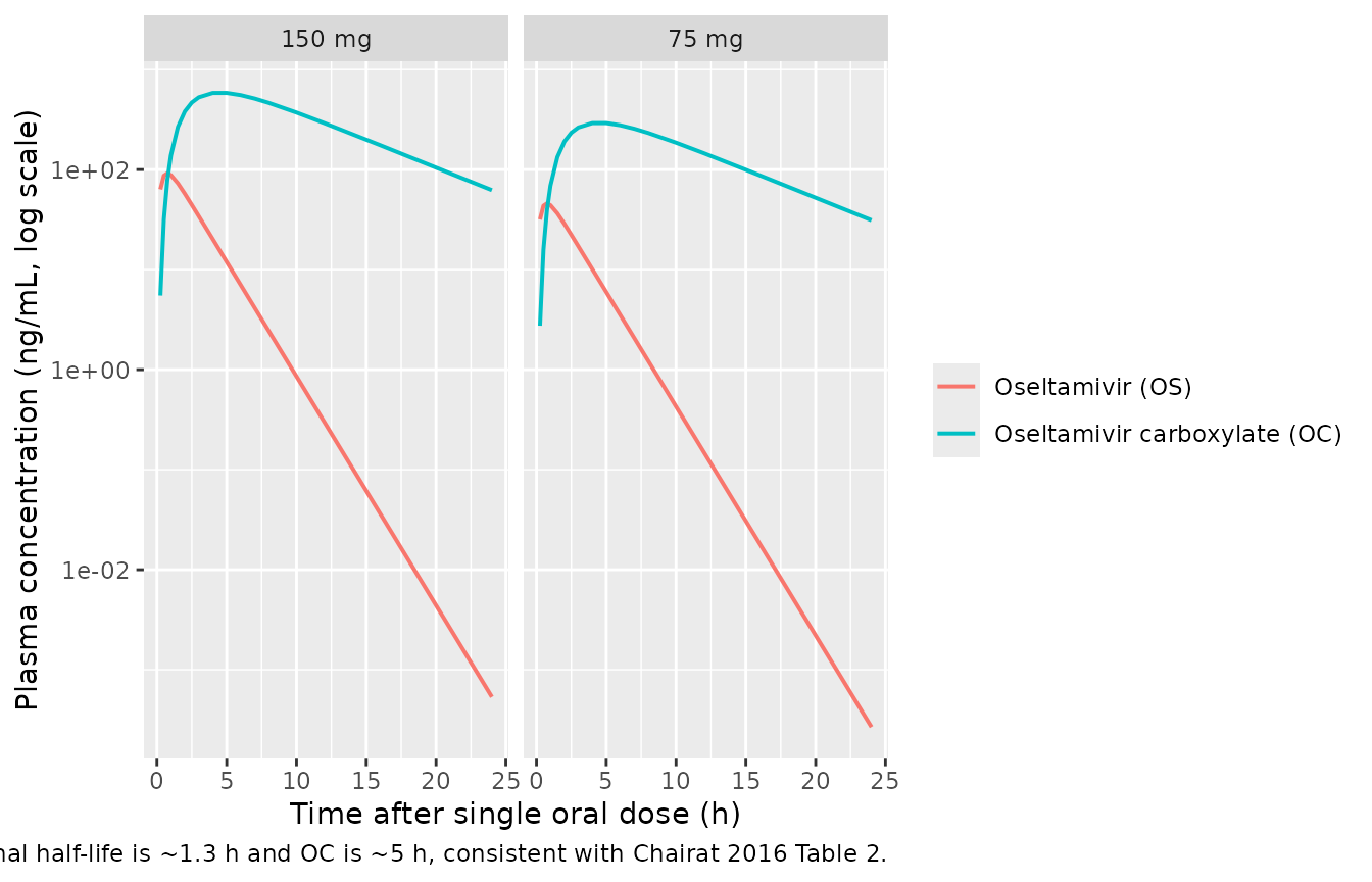
The typical-value profiles below illustrate the classic flip-flop shape of the parent-metabolite system: OS peaks within the first hour, OC peaks around 4-5 h and decays with the terminal slope of CL/FOC / V/FOC.
sim_typical |>
  dplyr::filter(time <= 24) |>
  tidyr::pivot_longer(c(Cc, Cc_oc), names_to = "analyte", values_to = "conc") |>
  dplyr::mutate(analyte = dplyr::recode(analyte,
                                          Cc = "Oseltamivir (OS)",
                                          Cc_oc = "Oseltamivir carboxylate (OC)")) |>
  ggplot(aes(time, conc, colour = analyte)) +
  geom_line(linewidth = 0.7) +
  facet_wrap(~ treatment) +
  scale_y_log10() +
  labs(x = "Time after single oral dose (h)",
       y = "Plasma concentration (ng/mL, log scale)",
       colour = NULL,
       caption = paste(
         "Chairat 2016 typical-value profiles (CLCR(FFM) = 73 mL/min;",
         "all etas = 0). The OS terminal half-life is ~1.3 h and OC is",
         "~5 h, consistent with Chairat 2016 Table 2."
       ))
A median-with-90% band gives a quick VPC-style check of the stochastic cohort:
sim |>
  dplyr::filter(time <= 24) |>
  tidyr::pivot_longer(c(Cc, Cc_oc), names_to = "analyte", values_to = "conc") |>
  dplyr::mutate(analyte = dplyr::recode(analyte,
                                          Cc = "Oseltamivir (OS)",
                                          Cc_oc = "Oseltamivir carboxylate (OC)")) |>
  dplyr::group_by(time, treatment, analyte) |>
  dplyr::summarise(
    Q05 = quantile(conc, 0.05, na.rm = TRUE),
    Q50 = quantile(conc, 0.50, na.rm = TRUE),
    Q95 = quantile(conc, 0.95, na.rm = TRUE),
    .groups = "drop"
  ) |>
  ggplot(aes(time, Q50, colour = analyte, fill = analyte)) +
  geom_ribbon(aes(ymin = Q05, ymax = Q95), alpha = 0.20, colour = NA) +
  geom_line(linewidth = 0.7) +
  facet_grid(analyte ~ treatment, scales = "free_y") +
  scale_y_log10() +
  labs(x = "Time (h)", y = "Plasma concentration (ng/mL, log scale)",
       colour = NULL, fill = NULL,
       caption = "Median (90% band) over the virtual cohort, first 24 h.")
#> Warning in scale_y_log10(): log-10 transformation introduced infinite values.
#> log-10 transformation introduced infinite values.
#> log-10 transformation introduced infinite values.
#> log-10 transformation introduced infinite values.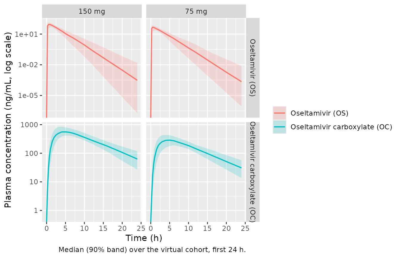
PKNCA validation
Single-dose NCA for the parent and the metabolite, computed per dose group. PKNCA runs are split per analyte because they share the same dose records but different concentration columns.
# Parent (OS) concentration frame: keep the column named Cc until the
# rename inside the PKNCA call. Add a time = 0 row defensively
# (extravascular pre-dose Cc = 0); see pknca-recipes.md.
sim_nca_parent <- sim |>
  dplyr::filter(!is.na(Cc)) |>
  dplyr::select(id, time, Cc, treatment)

sim_nca_parent <- dplyr::bind_rows(
  sim_nca_parent,
  sim_nca_parent |> dplyr::distinct(id, treatment) |>
    dplyr::mutate(time = 0, Cc = 0)
) |>
  dplyr::distinct(id, treatment, time, .keep_all = TRUE) |>
  dplyr::arrange(id, treatment, time)

# Metabolite (OC) concentration frame: same shape with Cc_oc.
sim_nca_oc <- sim |>
  dplyr::filter(!is.na(Cc_oc)) |>
  dplyr::select(id, time, Cc_oc, treatment)

sim_nca_oc <- dplyr::bind_rows(
  sim_nca_oc,
  sim_nca_oc |> dplyr::distinct(id, treatment) |>
    dplyr::mutate(time = 0, Cc_oc = 0)
) |>
  dplyr::distinct(id, treatment, time, .keep_all = TRUE) |>
  dplyr::arrange(id, treatment, time)

dose_df <- events |>
  dplyr::filter(evid == 1) |>
  dplyr::select(id, time, amt, treatment)

conc_obj_parent <- PKNCA::PKNCAconc(sim_nca_parent,
                                     Cc ~ time | treatment + id,
                                     concu = "ng/mL", timeu = "h")
#> Warning in assert_conc(conc, any_missing_conc = any_missing_conc): Negative
#> concentrations found
conc_obj_oc     <- PKNCA::PKNCAconc(sim_nca_oc,
                                     Cc_oc ~ time | treatment + id,
                                     concu = "ng/mL", timeu = "h")
dose_obj <- PKNCA::PKNCAdose(dose_df, amt ~ time | treatment + id,
                             doseu = "mg")

intervals <- data.frame(
  start     = 0,
  end       = 24,
  cmax      = TRUE,
  tmax      = TRUE,
  auclast   = TRUE,
  half.life = TRUE
)

nca_parent <- PKNCA::pk.nca(PKNCA::PKNCAdata(conc_obj_parent, dose_obj,
                                              intervals = intervals))
nca_oc     <- PKNCA::pk.nca(PKNCA::PKNCAdata(conc_obj_oc,     dose_obj,
                                              intervals = intervals))
Comparison against published NCA (Chairat 2016 Table 2)
Chairat 2016 Table 2 reports median NCA secondary parameters separately for non-obese and obese subjects at each dose. Because the formal final model (the one packaged here) does NOT retain an obesity covariate – the full-covariate analysis indicated a small (~25%) effect on CL/FOS and (~20%) on V/FOS that did not survive backward elimination at P < 0.001 – the comparison below uses the non-obese Table 2 medians as the reference (CLCR(FFM) in non-obese was closer to the population median used as the model’s centering value). The corresponding obese-group NCA values are higher for CL/FOS and V/FOS by the percentages noted in the source paper and are intentionally NOT matched by the packaged model.
published_parent <- tibble::tribble(
  ~treatment, ~cmax, ~tmax, ~auclast, ~half.life,
  "75 mg",    45.1,  0.819,      142,       1.42,
  "150 mg",   103,   0.630,      285,       1.27
)

cmp_parent <- nlmixr2lib::ncaComparisonTable(
  simulated = nca_parent,
  reference = published_parent,
  by        = "treatment",
  units     = c(cmax = "ng/mL", auclast = "ng*h/mL",
                tmax = "h",     half.life = "h"),
  tolerance_pct = 20
)

knitr::kable(
  cmp_parent,
  caption = paste(
    "Oseltamivir (OS): simulated vs Chairat 2016 Table 2 non-obese medians.",
    "* differs from reference by >20%."
  ),
  align = c("l", "l", "r", "r", "r")
)| NCA parameter | treatment | Reference | Simulated | % diff |
|---|---|---|---|---|
| Cmax (ng/mL) | 75 mg | 45.1 | 47.6 | +5.6% |
| Cmax (ng/mL) | 150 mg | 103 | 89.4 | -13.2% |
| Tmax (h) | 75 mg | 0.819 | 0.75 | -8.4% |
| Tmax (h) | 150 mg | 0.63 | 0.75 | +19.0% |
| AUClast (ng*h/mL) | 75 mg | 142 | 123 | -13.5% |
| AUClast (ng*h/mL) | 150 mg | 285 | 243 | -14.7% |
| t½ (h) | 75 mg | 1.42 | 1.3 | -8.2% |
| t½ (h) | 150 mg | 1.27 | 1.23 | -3.0% |
published_oc <- tibble::tribble(
  ~treatment, ~cmax, ~tmax, ~auclast, ~half.life,
  "75 mg",    266,   4.88,      3160,       5.45,
  "150 mg",   558,   4.47,      6320,       5.45
)

cmp_oc <- nlmixr2lib::ncaComparisonTable(
  simulated = nca_oc,
  reference = published_oc,
  by        = "treatment",
  units     = c(cmax = "ng/mL", auclast = "ng*h/mL",
                tmax = "h",     half.life = "h"),
  tolerance_pct = 20
)

knitr::kable(
  cmp_oc,
  caption = paste(
    "Oseltamivir carboxylate (OC): simulated vs Chairat 2016 Table 2",
    "non-obese medians. * differs from reference by >20%."
  ),
  align = c("l", "l", "r", "r", "r")
)| NCA parameter | treatment | Reference | Simulated | % diff |
|---|---|---|---|---|
| Cmax (ng/mL) | 75 mg | 266 | 288 | +8.2% |
| Cmax (ng/mL) | 150 mg | 558 | 563 | +0.9% |
| Tmax (h) | 75 mg | 4.88 | 5 | +2.5% |
| Tmax (h) | 150 mg | 4.47 | 5 | +11.9% |
| AUClast (ng*h/mL) | 75 mg | 3160 | 3310 | +4.8% |
| AUClast (ng*h/mL) | 150 mg | 6320 | 6620 | +4.8% |
| t½ (h) | 75 mg | 5.45 | 5.39 | -1.2% |
| t½ (h) | 150 mg | 5.45 | 5.42 | -0.6% |
Assumptions and deviations
IOV encoded as IIV. Chairat 2016 Table 1 reports interoccasion variability (IOV) on
ka(98.7% CV),V/FOS(18.6% CV), andkm(43.2% CV). rxode2 / nlmixr2 simulation in a popPK validation context generally uses a single occasion per subject, so the packaged model encodes these components as additional IIV terms (independent log-normaletas on each parameter). For simulating a single cross-over arm or a single dosing occasion this approximation gives a variance magnitude matching the published estimates. A workflow that needs explicit occasion-to-occasion variation within a subject (e.g. re-fitting the cross-over data) would need to layer additional IOV etas keyed on an OCC indicator beyond what is encoded here.Obesity covariate intentionally NOT in the formal model. The full covariate analysis in Chairat 2016 (Results paragraph on Figure 4 and Discussion) identified ~25% higher apparent CL/FOS, ~20% higher V/FOS, and ~10% higher CL/FOC in obese subjects, but these did NOT survive backward elimination at P < 0.001 due to the small sample size (n = 24). The packaged model reproduces the formal final model and therefore does not include an obesity / BMI / fat-mass effect. The Table 2 obese-group NCA medians are correspondingly NOT matched by the model; the comparison table above uses the non-obese Table 2 medians, whose CLCR(FFM) is closer to the population median (73 mL/min) used for the cohort here.
CLCR(FFM) reference value. Chairat 2016 Methods describes continuous covariates as “centred on the median value of the population” and Equation 11 reads
CL/FOC = 20.6 * [1 + 0.0384 * (CLCR(FFM) - 73)/10]. The 73 mL/min centring value is taken from Equation 11 verbatim. The Discussion paragraph on renal-impairment extrapolation also references a “normal CLCR(FFM) of 75 mL/min” – this is the rounded reference used in the dose-impact discussion, not the centring value used in the covariate equation.Residual error encoding. The paper used NONMEM “additive on log-transformed concentration” residuals (sd = 0.431 for OS, sd = 0.161 for OC). This corresponds to a log-normal residual on the natural scale and is encoded here via
Cc ~ lnorm(expSd)andCc_oc ~ lnorm(expSd_oc).Concentration units. The paper fitted the model in molar units (Methods paragraph 1 - concentrations were converted to equivalent molar concentrations and natural-log transformed before fitting). The reported parameter table (Table 1) is dimensionless with respect to mass vs molar units (CL/F and V/F have units of L/h and L only). The packaged model expresses dose in mg and computes
Cc = 1000 * central / vc, putting concentrations in ng/mL to match the reported units of Chairat 2016 Table 2 (Cmax, AUC) directly.Time-zero row added defensively in PKNCA blocks. The simulation grid above already includes
time = 0(pre-dose, Cc = 0 for the extravascular dose), but thebind_rows()recipe is kept for robustness in case the grid is later modified. PKNCA’sRequesting an AUC range starting (0) before the first measurementwarning would otherwise fire once per subject if the grid does not carry a time-zero observation.