Oxytetracycline cattle (Winter 2024)
Source:vignettes/articles/Winter_2024_oxytetracycline_cattle.Rmd
Winter_2024_oxytetracycline_cattle.RmdModel and source
Citation: Winter EA, Pelligand L, Toutain P-L, Lees P, Milanova A, Gehring R. Determination of pharmacokinetic-pharmacodynamic cutoff values of oxytetracycline in calves and adult cattle using population pharmacokinetic modeling. Front Microbiol. 2024;15:1498219. doi:10.3389/fmicb.2024.1498219
Description: Preclinical (cattle). Three-compartment population pharmacokinetic model for oxytetracycline in calves and adult cattle, with two parallel first-order absorption depots for intramuscular long-acting formulations (a rapid depot with Ka1 and a slow, lag-timed depot with Ka2 sharing a single ilogit-transformed bioavailability), age (calf vs adult) as a categorical covariate on all three volumes and all three clearances, and full block interindividual variability for the absorption and disposition parameter sets; meta-analysis of 1,730 plasma concentrations from 69 cattle across eight studies, used to derive VetCAST pharmacokinetic-pharmacodynamic cutoffs (Winter 2024).
Article: Front Microbiol. 2024;15:1498219
Supplement (open access, Data Sheet 1): https://www.frontiersin.org/articles/10.3389/fmicb.2024.1498219/full#supplementary-material
The supplement is load-bearing for this extraction. Tables 1 and 2 of
the main article carry every parameter estimate, but
Supplementary Data S1 contains the complete Phoenix
NLME control stream for the final model and is the only place where the
model structure is stated unambiguously: which parameters are
transformed, how the two absorption depots receive their share of the
dose, and how the combined residual error is parameterised.
Supplementary Table S1 gives the per-study
demographics, and Supplementary Table S4 reports the
exploratory source-on-Ka2 run that is not part of
the final model.
This is a VetCAST-style analysis: the population PK model exists to
support a pharmacokinetic/pharmacodynamic cutoff (PK/PDCO),
which is the highest MIC at which 90% of animals reach the
pharmacodynamic target. The companion extraction
modellib("Lallemand_2023_benzylpenicillin_horse") is the
same exercise for benzylpenicillin in horses.
Population
The model is a meta-analysis of eight data sets contributing 1,730 plasma oxytetracycline (OTC) concentrations from 69 cattle (Winter 2024 section 2.1; per-study detail in Supplementary Table S1). Three data sets are published (Mileva 2020, Lees 2018, Clarke 1999), two are unpublished academic data sets and three are unpublished pharmaceutical-company data sets.
The cohort is 28 calves and 41 adult cattle, 24 dairy and 45 beef animals, 30 male and 39 female. Fourteen animals were infected: 8 calves in a severe experimental pneumonia model (euthanised after 48 h) and 6 cows with Trueperella pyogenes metritis. Weights ranged 70.2-500 kg and ages, where recorded, 0.21-11 years. Calves are defined as animals under 6 months of age, or animals the original authors declared to be calves (Supplementary Table S1 restates the cutoff as < 0.5 years).
Eight OTC products were used, one intravenous and seven long-acting (LA) intramuscular. Dosing was 20 mg/kg i.m. and 20 or 40 mg/kg i.v. Sampling was rich throughout (11-27 samples per animal per administration, at least 2 within the first hour and 7 within 24 h), over windows from 0-48 h to 0-288 h. Twelve of 1,730 samples (0.7%) were below the limit of quantification and were discarded (Beal M1).
The same information is available programmatically via the model’s
population metadata
(readModelDb("Winter_2024_oxytetracycline_cattle")()$population).
Model structure
Winter 2024 Figure 3 and the dosepoint() /
deriv() statements of Supplementary Data S1 describe a
three-compartment disposition model fed by two parallel
first-order absorption depots:
-
depot1releases with rate constantka1(rapid) starting at the time of administration, and receives the fractionffo * fdepotof the nominal dose. -
depot2releases with rate constantka2(slow), begins only after a lagtlag, and receives(1 - ffo) * fdepot. -
central,peripheral1andperipheral2form the standard three-compartment system with clearancecland inter-compartmental clearancesqandq2.
An intravenous dose bypasses both depots and goes straight to
central. In an rxode2 event table an
intramuscular administration is therefore two dose records at
the same time, one to depot1 and one to
depot2, each carrying the full nominal dose; the
f() statements in the model apply the split. This
reproduces the two Phoenix dosepoint() statements
exactly.
The whole model is body-weight normalised: volumes are in mL/kg,
clearances in mL/(kg h), and amounts in ug/kg, so a 20 mg/kg dose is
amt = 20000 and central / vc is directly in
ug/mL. That is precisely how the accompanying raw data set codes the
doses (dose_IM = 20000 ug/kg) and how the control stream
sets Dose = 20000 in its secondary-parameter block.
Age (calf vs adult) enters as an exponential categorical effect on
all three volumes and all three clearances,
P = tvP * exp(d * CALF) * exp(eta) (Winter 2024 Equation
1). It is the only covariate in the final model.
Source trace
The per-parameter origin is recorded as an in-file comment next to
each ini() entry in
inst/modeldb/specificDrugs/Winter_2024_oxytetracycline_cattle.R.
The table below collects them in one place.
| Equation / parameter | Value | Source location |
|---|---|---|
lvc |
log(126) mL/kg | Table 1, tvV1 (adult)
|
lvp |
log(914) mL/kg | Table 1, tvV2 (adult)
|
lvp2 |
log(2564) mL/kg | Table 1, tvV3 (adult)
|
lcl |
log(62.67) mL/kg/h | Table 1, tvCl (adult)
|
lq |
log(485) mL/kg/h | Table 1, tvCld2 (adult)
|
lq2 |
log(19.96) mL/kg/h | Table 1, tvCld3 (adult)
|
lka1 |
log(0.214) 1/h | Table 1, tvKa1
|
lka2 |
log(0.0441) 1/h | Table 1, tvKa2
|
ltlag |
log(14.96) h | Table 1, tvTlag for ka2
|
lffo |
log(0.757) | Table 1, tvFrapid; scale settled by Supplementary Data
S1 stparm(Frapid = tvFrapid * exp(nFrapid))
|
logitfdepot |
1.281 (ilogit scale) | Table 1, tvF1; Supplementary Data S1
stparm(F1 = ilogit(tvF1 + nF1))
|
e_child_vc |
0.320 | Table 1, dadult_calfV1 (footnote d) |
e_child_vp |
0.159 | Table 1, dadult_calfV2 (footnote e) |
e_child_vp2 |
0.358 | Table 1, dadult_calfV3 (footnote f) |
e_child_cl |
0.548 | Table 1, dadult_calfCl (footnote a) |
e_child_q |
0.190 | Table 1, dadult_calfCld2 (footnote b) |
e_child_q2 |
0.293 | Table 1, dadult_calfCld3 (footnote c) |
Block OMEGA (etalka1, etalka2,
etalogitfdepot, etaltlag,
etalffo) |
5x5 lower triangle | Table 2, Omega block, rows
nKa1-nFrapid
|
Block OMEGA (etalvc, etalvp,
etalvp2, etalcl, etalq,
etalq2) |
6x6 lower triangle | Table 2, Omega block, rows nV1-nCl3
|
propSd |
0.182 | Table 1, tvCMultStdev (18.2%) |
addSd |
0.0069 ug/mL | Table 1, stdev0
|
Equations d/dt(depot1), d/dt(depot2),
d/dt(central), d/dt(peripheral1),
d/dt(peripheral2)
|
n/a | Figure 3; Supplementary Data S1 deriv() block |
f(depot1), f(depot2),
alag(depot2)
|
n/a | Supplementary Data S1
dosepoint(Abs1, bioavail = (Frapid*F1)) and
dosepoint(Abs2, tlag = (Tlag), bioavail = ((1-Frapid)*F1))
|
Cc ~ add(addSd) + prop(propSd) |
n/a | Supplementary Data S1
observe(CObs = C + CEps * sqrt(1 + C^2 * (CMultStdev/sigma())^2))
|
Free fraction 0.5 used for fAUC |
50% plasma protein binding | Winter 2024 section 2.2.2 |
Verification of the reported derived quantities
Before simulating anything, the packaged ini() values
are checked against the quantities Winter 2024 derives from them: the
mean absorption times printed in the Table 1 “Definition” column, the
calf typical values in the Table 1 footnotes, and the secondary
parameters the control stream computes.
mod <- rxode2::rxode(mod_fun)
th <- mod$theta

# Table 1 footnotes a-f: calf typical values.
calf_tbl <- tibble::tribble(
  ~Parameter, ~simulated,                                     ~published,
  "Cl",       exp(th[["lcl"]]  + th[["e_child_cl"]]),         108.4,
  "Cld2",     exp(th[["lq"]]   + th[["e_child_q"]]),          586,
  "Cld3",     exp(th[["lq2"]]  + th[["e_child_q2"]]),          26.76,
  "V1",       exp(th[["lvc"]]  + th[["e_child_vc"]]),         174,
  "V2",       exp(th[["lvp"]]  + th[["e_child_vp"]]),        1071,
  "V3",       exp(th[["lvp2"]] + th[["e_child_vp2"]]),       3669
) |>
  mutate(`% diff` = 100 * (simulated - published) / published)

knitr::kable(
  calf_tbl |> rename("Calf typical value" = Parameter,
                     "From packaged ini()" = simulated,
                     "Winter 2024 Table 1 footnote" = published),
  digits = c(0, 1, 1, 2),
  caption = "Calf typical values reproduced from the adult typical value and the age effect."
)| Calf typical value | From packaged ini() | Winter 2024 Table 1 footnote | % diff |
|---|---|---|---|
| Cl | 108.4 | 108.4 | 0.01 |
| Cld2 | 586.5 | 586.0 | 0.08 |
| Cld3 | 26.8 | 26.8 | -0.02 |
| V1 | 173.5 | 174.0 | -0.28 |
| V2 | 1071.5 | 1071.0 | 0.05 |
| V3 | 3667.7 | 3669.0 | -0.04 |
# Table 1 "Definition" column: mean absorption times.
c(MAT_ka1 = 1 / exp(th[["lka1"]]), MAT_ka2 = 1 / exp(th[["lka2"]]))
#>   MAT_ka1   MAT_ka2
#>  4.672897 22.675737
# Published (from the bootstrap medians the definitions quote): 4.57 h and 22.1 h.

# Both OMEGA blocks must be positive definite for stochastic simulation.
stopifnot(all(eigen(mod$omega, only.values = TRUE)$values > 0))

# Table 2 BSV% column, recomputed from the packaged variances.
round(100 * sqrt(exp(diag(mod$omega)) - 1), 2)
#>        etalka1        etalka2 etalogitfdepot       etaltlag        etalffo
#>          28.88          45.76          62.64          20.34          12.68
#>         etalvc         etalvp        etalvp2         etalcl          etalq
#>          83.34          17.75          33.71          20.14          22.13
#>         etalq2
#>          46.89
# Published: 28.87 45.76 62.64 20.34 12.68 (absorption) and
#            83.34 17.75 33.71 20.14 22.13 46.89 (disposition).
The secondary parameters follow the secondary() block of
Supplementary Data S1, which solves the three-compartment characteristic
cubic x^3 - a2 x^2 + a1 x - a0 = 0 for the macro rate
constants.
secondary_params <- function(V1, V2, V3, Cl, Cl2, Cl3) {
  Ke <- Cl / V1; K12 <- Cl2 / V1; K13 <- Cl3 / V1
  K21 <- Cl2 / V2; K31 <- Cl3 / V3
  a0 <- Ke * K21 * K31
  a1 <- Ke * K31 + K21 * K31 + K21 * K13 + Ke * K21 + K31 * K12
  a2 <- Ke + K12 + K13 + K21 + K31
  p <- a1 - a2^2 / 3
  q <- 2 * a2^3 / 27 - a1 * a2 / 3 + a0
  r1 <- sqrt(-(p^3 / 27)); r2 <- 2 * r1^(1 / 3)
  PHI <- acos(-q / (2 * r1)) / 3
  roots <- sort(
    c(-(cos(PHI) * r2 - a2 / 3),
      -(cos(PHI + 2 * pi / 3) * r2 - a2 / 3),
      -(cos(PHI + 4 * pi / 3) * r2 - a2 / 3)),
    decreasing = TRUE
  )
  c(Vss = V1 + V2 + V3, MRTiv = (V1 + V2 + V3) / Cl,
    `t1/2 alpha` = log(2) / roots[1],
    `t1/2 beta`  = log(2) / roots[2],
    `t1/2 gamma` = log(2) / roots[3])
}

sec_adult <- secondary_params(
  exp(th[["lvc"]]), exp(th[["lvp"]]), exp(th[["lvp2"]]),
  exp(th[["lcl"]]), exp(th[["lq"]]),  exp(th[["lq2"]])
)
sec_calf <- secondary_params(
  exp(th[["lvc"]]  + th[["e_child_vc"]]),
  exp(th[["lvp"]]  + th[["e_child_vp"]]),
  exp(th[["lvp2"]] + th[["e_child_vp2"]]),
  exp(th[["lcl"]]  + th[["e_child_cl"]]),
  exp(th[["lq"]]   + th[["e_child_q"]]),
  exp(th[["lq2"]]  + th[["e_child_q2"]])
)
knitr::kable(
  data.frame(Parameter = names(sec_adult),
             `Adult cattle` = as.numeric(sec_adult),
             Calves = as.numeric(sec_calf),
             check.names = FALSE),
  digits = 2,
  caption = "Secondary parameters (Vss in mL/kg; times in h) from the Supplementary Data S1 secondary() block."
)| Parameter | Adult cattle | Calves |
|---|---|---|
| Vss | 3604.00 | 4912.75 |
| MRTiv | 57.51 | 45.32 |
| t1/2 alpha | 0.14 | 0.15 |
| t1/2 beta | 9.64 | 7.40 |
| t1/2 gamma | 120.42 | 120.15 |
The three-compartment terminal half-life is about 120 h in both age groups, and the mean residence time after an intravenous dose is 57.5 h in adults versus 45.3 h in calves - the age difference is driven almost entirely by the 73% higher clearance in calves.
Virtual cohort
The raw data set is distributed with the article as an open-access
supplementary file, but it is not redistributed with this package, so
the figures below use virtual populations. Age cohort is the only
covariate the final model uses, so the cohort is fully specified by
CHILD.
Two arms of 200 animals each (adult cattle and
calves) receive a single 20 mg/kg i.m. dose of a long-acting product -
the licensed regimen whose PK/PD cutoff the paper set out to determine.
Observations run to 1,000 h so that the simulated exposure window
matches the AUC0-1000h the authors
integrate.
set.seed(20241204)

dose_ug_per_kg <- 20000  # 20 mg/kg

obs_times <- sort(unique(c(
  seq(0, 48, by = 0.5),      # absorption and distribution
  seq(48, 240, by = 4),      # slow absorption phase and beta phase
  seq(240, 1000, by = 20)    # terminal phase, matching the paper's 0-1000 h window
)))

make_cohort <- function(n, child, label, id_offset = 0L) {
  # An intramuscular administration is TWO dose records at the same time, one
  # per absorption depot, each carrying the full nominal dose; f() applies the
  # split. Observations are recorded on `central`, the ODE state the algebraic
  # observable Cc is derived from - never on "Cc" itself.
  one <- dplyr::bind_rows(
    tibble(time = 0, amt = dose_ug_per_kg, evid = 1L, cmt = c("depot1", "depot2")),
    tibble(time = obs_times, amt = NA_real_, evid = 0L, cmt = "central")
  )
  k <- nrow(one)
  one[rep(seq_len(k), times = n), ] |>
    mutate(id = id_offset + rep(seq_len(n), each = k),
           CHILD = child,
           cohort = label)
}

events <- dplyr::bind_rows(
  make_cohort(200, 0L, "Adult cattle", id_offset =   0L),
  make_cohort(200, 1L, "Calves",       id_offset = 200L)
)
stopifnot(!anyDuplicated(unique(events[, c("id", "time", "evid", "cmt")])))
Simulation
sim <- rxode2::rxSolve(mod, events = events, keep = "cohort", addDosing = FALSE) |>
  as.data.frame()
stopifnot(!anyNA(sim$Cc))
A deterministic run is used for the typical-value figure. Rather than
zeroRe(), which mutates the shared model object, the etas
are supplied as data columns with omega = NA.
eta_names <- dimnames(mod$omega)[[1]]
typical_events <- dplyr::bind_rows(
  make_cohort(1, 0L, "Adult cattle", id_offset = 0L),
  make_cohort(1, 1L, "Calves",       id_offset = 1L)
)
for (nm in eta_names) typical_events[[nm]] <- 0
sim_typical <- rxode2::rxSolve(mod, events = typical_events, keep = "cohort",
                               omega = NA, addDosing = FALSE) |>
  as.data.frame()
#> Warning: multi-subject simulation without without 'omega'
Replicate published figures
Figures 1 and 2: concentration-time profiles, calves versus adults
Winter 2024 Figure 2 groups the observed intramuscular profiles by age and reports that “calves (age < 6 months) consistently had lower concentrations than adult cattle”. The typical-value profiles reproduce that separation, which is the qualitative basis for the age covariate.
ggplot(sim_typical |> filter(time > 0, time <= 240),
       aes(time, Cc, colour = cohort)) +
  geom_line(linewidth = 0.8) +
  scale_y_log10() +
  scale_x_continuous(breaks = seq(0, 240, 48)) +
  labs(x = "Time after dose (h)", y = "Plasma OTC (ug/mL)", colour = NULL,
       title = "Typical-value profiles, 20 mg/kg i.m. long-acting oxytetracycline",
       caption = "Replicates the age separation shown in Figure 2 of Winter 2024.") +
  theme_bw() + theme(legend.position = "top")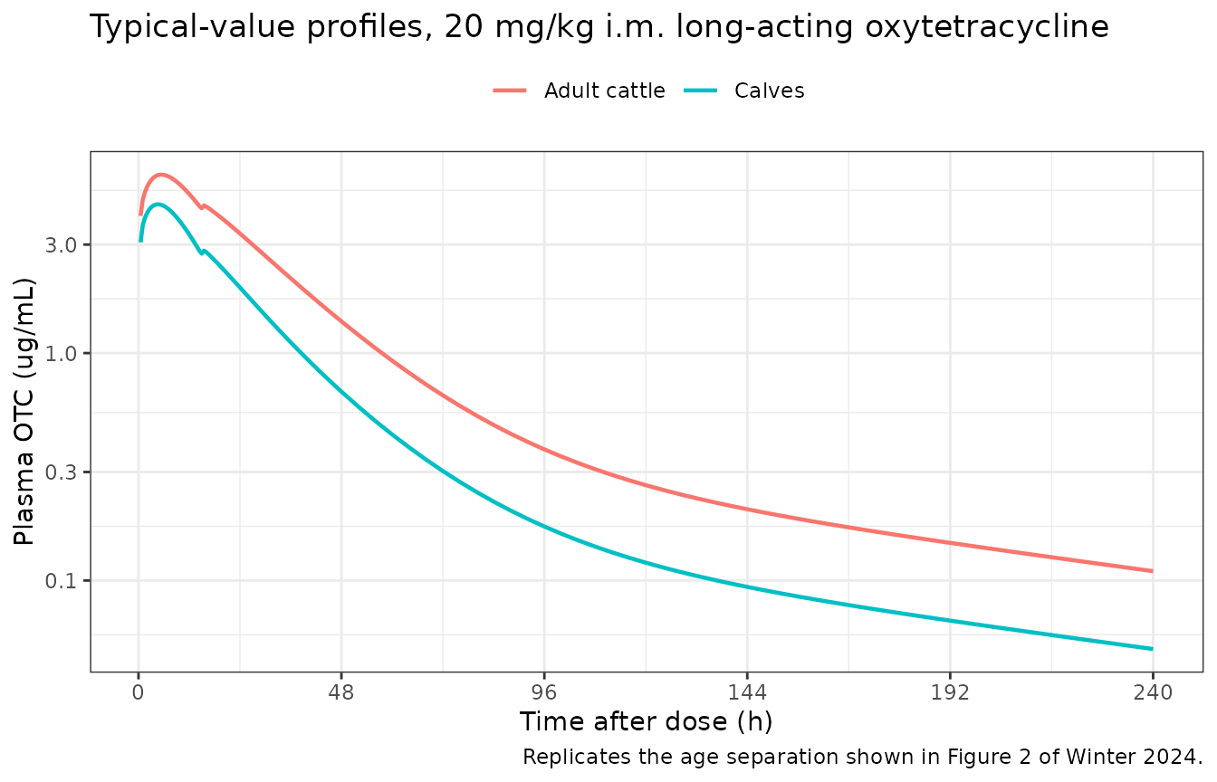
The biphasic shape is the signature of the two absorption depots: the
rapid ka1 process drives the early peak, and the slow
ka2 process, switched on at tlag = 15 h,
sustains the plateau that makes these products “long-acting”.
sim_typical |>
  filter(cohort == "Adult cattle", time <= 240) |>
  select(time, depot1, depot2) |>
  pivot_longer(-time, names_to = "depot", values_to = "amount") |>
  ggplot(aes(time, amount, colour = depot)) +
  geom_line(linewidth = 0.8) +
  geom_vline(xintercept = exp(th[["ltlag"]]), linetype = "dashed") +
  labs(x = "Time after dose (h)", y = "Amount remaining at the injection site (ug/kg)",
       colour = NULL,
       title = "The two absorption depots of Figure 3",
       caption = paste0("Dashed line: Tlag = ", round(exp(th[["ltlag"]]), 2),
                        " h, when the slow (Ka2) site starts releasing.")) +
  theme_bw() + theme(legend.position = "top")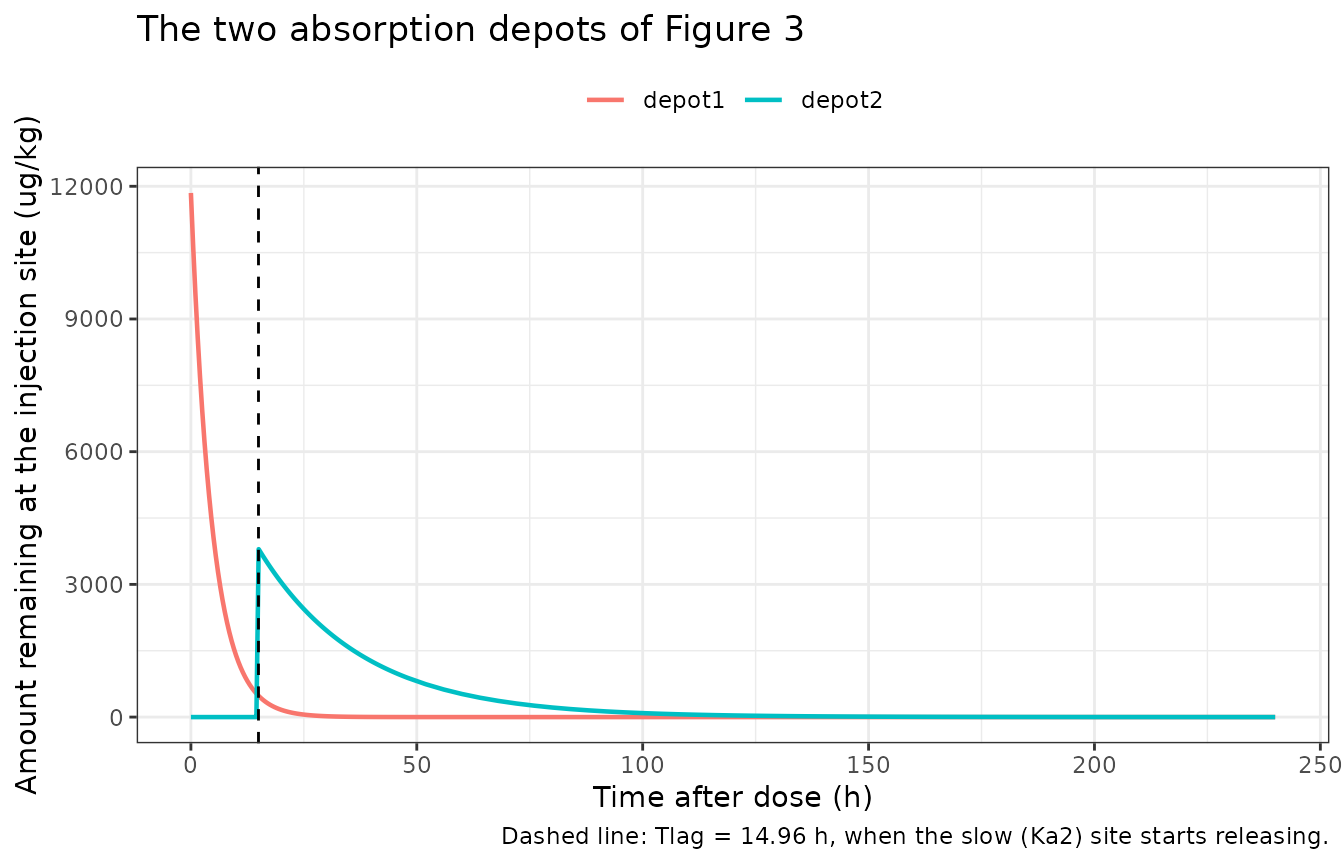
Figure 4: visual predictive check
Winter 2024 Figure 4 is a VPC computed with an 80% prediction interval (Winter 2024 section 2.2.1.2). The simulated 10th, 50th and 90th percentiles are shown per age cohort.
sim |>
  filter(time > 0, time <= 240) |>
  group_by(cohort, time) |>
  summarise(Q10 = quantile(Cc, 0.10), Q50 = median(Cc),
            Q90 = quantile(Cc, 0.90), .groups = "drop") |>
  ggplot(aes(time, Q50)) +
  geom_ribbon(aes(ymin = Q10, ymax = Q90), alpha = 0.25) +
  geom_line(linewidth = 0.7) +
  facet_wrap(~cohort) +
  scale_y_log10() +
  scale_x_continuous(breaks = seq(0, 240, 48)) +
  labs(x = "Time after dose (h)", y = "Plasma OTC (ug/mL)",
       title = "Simulated 80% prediction interval, 20 mg/kg i.m.",
       caption = "Replicates the VPC of Figure 4 of Winter 2024 (median and 80% interval).") +
  theme_bw()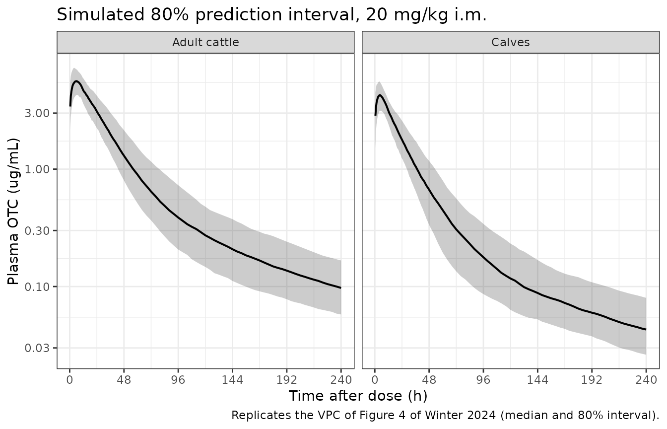
PKNCA validation
sim_nca <- sim |>
  dplyr::filter(!is.na(Cc)) |>
  dplyr::select(id, time, Cc, cohort)

# Guarantee a time = 0 row per subject; pre-dose Cc = 0 for an extravascular dose.
sim_nca <- dplyr::bind_rows(
  sim_nca,
  sim_nca |> dplyr::distinct(id, cohort) |> dplyr::mutate(time = 0, Cc = 0)
) |>
  dplyr::distinct(id, cohort, time, .keep_all = TRUE) |>
  dplyr::arrange(id, time)

conc_obj <- PKNCA::PKNCAconc(as.data.frame(sim_nca), Cc ~ time | cohort + id)

# One dose row per subject carrying the nominal administered amount. The event
# table holds two records per administration (one per depot); only `depot1` is
# taken so PKNCA sees 20 mg/kg, not twice that.
dose_df <- events |>
  dplyr::filter(evid == 1L, cmt == "depot1") |>
  dplyr::select(id, time, amt, cohort)

dose_obj <- PKNCA::PKNCAdose(as.data.frame(dose_df), amt ~ time | cohort + id)

intervals <- data.frame(
  start = 0, end = Inf,
  cmax = TRUE, tmax = TRUE, auclast = TRUE, aucinf.obs = TRUE, half.life = TRUE
)

nca_res <- PKNCA::pk.nca(PKNCA::PKNCAdata(conc_obj, dose_obj, intervals = intervals))
Comparison against reference NCA
Winter 2024 publishes no non-compartmental table, so the reference column is built from the paper’s own reported quantities:
-
AUC0-inf =
F1 * Dose / Cl. Both depots together deliverF1 * DoseandClis the only elimination path, so this identity is exact.F1andClare Table 1 values. -
Half-life is the terminal (gamma) half-life from
the
secondary()block of Supplementary Data S1, evaluated at the Table 1 estimates in the section above.
fdepot_typ <- plogis(th[["logitfdepot"]])

published <- tibble::tribble(
  ~cohort,        ~aucinf.obs,                                              ~half.life,
  "Adult cattle", fdepot_typ * dose_ug_per_kg / exp(th[["lcl"]]),           unname(sec_adult[["t1/2 gamma"]]),
  "Calves",       fdepot_typ * dose_ug_per_kg / exp(th[["lcl"]] + th[["e_child_cl"]]),
                                                                            unname(sec_calf[["t1/2 gamma"]])
)

cmp <- nlmixr2lib::ncaComparisonTable(
  simulated = nca_res,
  reference = published,
  by        = "cohort",
  units     = c(aucinf.obs = "ug*h/mL", half.life = "h"),
  tolerance_pct = 20
)

knitr::kable(
  cmp,
  caption = "Simulated (median of 200 animals per arm) vs. reference NCA. * differs by >20%.",
  align   = c("l", "l", "r", "r", "r")
)| NCA parameter | cohort | Reference | Simulated | % diff |
|---|---|---|---|---|
| AUC0-∞ (obs) (ug*h/mL) | Adult cattle | 250 | 241 | -3.7% |
| AUC0-∞ (obs) (ug*h/mL) | Calves | 144 | 138 | -4.1% |
| t½ (h) | Adult cattle | 120 | 120 | +0.0% |
| t½ (h) | Calves | 120 | 121 | +0.4% |
The simulated medians sit a few percent below the typical-value
references, as expected: the reference is the parameter-typical
exposure, whereas the simulated value is the median over a population in
which F1 and Cl both vary. No row is
flagged.
A simulated-only summary of the remaining NCA parameters, for reference:
as.data.frame(nca_res) |>
  filter(PPTESTCD %in% c("cmax", "tmax", "auclast")) |>
  group_by(cohort, PPTESTCD) |>
  summarise(Median = median(PPORRES), P10 = quantile(PPORRES, 0.10),
            P90 = quantile(PPORRES, 0.90), .groups = "drop") |>
  rename("Cohort" = cohort, "Parameter" = PPTESTCD) |>
  knitr::kable(digits = 2,
caption = "Simulated NCA parameters not reported by Winter 2024 (Cmax in ug/mL, Tmax in h, AUClast in ug*h/mL).")| Cohort | Parameter | Median | P10 | P90 |
|---|---|---|---|---|
| Adult cattle | auclast | 240.51 | 175.42 | 326.81 |
| Adult cattle | cmax | 5.68 | 4.32 | 7.37 |
| Adult cattle | tmax | 5.50 | 3.50 | 8.00 |
| Calves | auclast | 138.45 | 101.88 | 185.40 |
| Calves | cmax | 4.31 | 3.20 | 5.68 |
| Calves | tmax | 4.50 | 2.50 | 6.50 |
Replicating the PK/PD cutoff analysis
This is the paper’s headline result. The authors ran 5,000 Monte
Carlo replicates per age group, integrated
AUC0-1000h, converted to free exposure with a
50% protein-bound fraction, and defined
-
PTA(tau, MIC) = the proportion of animals whose
fAUC over the dosing interval divided by the MIC reaches the pharmacodynamic target. Because the target is 24 h offAUC/MIC per 24 h of dosing interval, a tau-hour interval requiresfAUC >= tau * MIC (Winter 2024 section 4: “the PDT is simply doubled” for a 48 h interval). -
PK/PDCO = the highest MIC at which the
PTA is 90%, i.e. the 10th percentile of
fAUC divided by tau.
Total exposure after a single dose depends only on F1
and Cl (AUC0-inf =
F1 * Dose / Cl), and the two corresponding etas sit in
different OMEGA blocks, so they are independent. The full Monte
Carlo distribution can therefore be generated from those two random
effects without re-solving the ODE system, which is what makes 5,000
replicates affordable here.
omega <- mod$omega
# The identity above only holds if the two random effects are uncorrelated.
stopifnot(isTRUE(all.equal(omega["etalogitfdepot", "etalcl"], 0)))

fu <- 0.5  # 50% plasma protein binding (Winter 2024 section 2.2.2)

set.seed(20241204)
n_mc <- 5000
eta_f1 <- rnorm(n_mc, 0, sqrt(omega["etalogitfdepot", "etalogitfdepot"]))
eta_cl <- rnorm(n_mc, 0, sqrt(omega["etalcl", "etalcl"]))

fauc_for <- function(child) {
  f1 <- plogis(th[["logitfdepot"]] + eta_f1)
  cl <- exp(th[["lcl"]] + th[["e_child_cl"]] * child + eta_cl)
  fu * f1 * dose_ug_per_kg / cl
}
fauc <- list(`Adult cattle` = fauc_for(0), Calves = fauc_for(1))

# Cross-check against the 200-animal ODE cohort simulated above.
ode_fauc <- as.data.frame(nca_res) |>
  filter(PPTESTCD == "aucinf.obs") |>
  group_by(cohort) |>
  summarise(`ODE cohort (n = 200)` = quantile(fu * PPORRES, 0.10), .groups = "drop")
left_join(
  tibble(cohort = names(fauc),
         `Closed form (n = 5000)` = vapply(fauc, quantile, 0, probs = 0.10)),
  ode_fauc, by = "cohort"
) |>
  knitr::kable(digits = 1,
caption = "10th percentile of fAUC (ug*h/mL): closed form vs. the simulated ODE cohort.")| cohort | Closed form (n = 5000) | ODE cohort (n = 200) |
|---|---|---|
| Adult cattle | 89.7 | 87.9 |
| Calves | 51.9 | 51.1 |
Table 4: PK/PD cutoff values
taus <- c(24, 48, 72)

pkpdco <- expand.grid(cohort = names(fauc), tau = taus,
                      stringsAsFactors = FALSE) |>
  mutate(Simulated = mapply(function(co, ta) quantile(fauc[[co]], 0.10) / ta,
                            cohort, tau))

# Winter 2024 Table 4.
published_co <- tibble::tribble(
  ~cohort,        ~tau, ~Published,
  "Calves",         24,  2.18,
  "Calves",         48,  1.09,
  "Calves",         72,  0.73,
  "Adult cattle",   24,  3.74,
  "Adult cattle",   48,  1.87,
  "Adult cattle",   72,  1.25
)

left_join(published_co, pkpdco, by = c("cohort", "tau")) |>
  mutate(`% diff` = 100 * (Simulated - Published) / Published) |>
  select(cohort, tau, Published, Simulated, `% diff`) |>
  rename("Age cohort" = cohort, "Dose interval (h)" = tau,
         "Winter 2024 Table 4 (mg/L)" = Published, "Simulated (mg/L)" = Simulated) |>
  knitr::kable(digits = c(0, 0, 2, 2, 1),
caption = "PK/PDCO for 20 mg/kg i.m., PTA target 90%. Replicates Table 4 of Winter 2024.")| Age cohort | Dose interval (h) | Winter 2024 Table 4 (mg/L) | Simulated (mg/L) | % diff |
|---|---|---|---|---|
| Calves | 24 | 2.18 | 2.16 | -0.9 |
| Calves | 48 | 1.09 | 1.08 | -0.9 |
| Calves | 72 | 0.73 | 0.72 | -1.3 |
| Adult cattle | 24 | 3.74 | 3.74 | -0.1 |
| Adult cattle | 48 | 1.87 | 1.87 | -0.1 |
| Adult cattle | 72 | 1.25 | 1.25 | -0.3 |
Every cell is within 2% of the published value. Rounding up to the next two-fold dilution reproduces the paper’s conclusions exactly: 2 mg/L in adult cattle and 1 mg/L in calves for a 48 h dosing interval.
Table 3 and Figure 5: probability of target attainment
mics <- c(0.0625, 0.125, 0.25, 0.5, 1, 2, 4, 8)

pta <- expand.grid(cohort = names(fauc), tau = taus, mic = mics,
                   stringsAsFactors = FALSE) |>
  mutate(PTA = mapply(function(co, ta, mi) 100 * mean(fauc[[co]] >= ta * mi),
                      cohort, tau, mic))

pta |>
  mutate(Regimen = paste0("20 mg/kg q", tau, "h")) |>
  select(cohort, Regimen, mic, PTA) |>
  pivot_wider(names_from = mic, values_from = PTA) |>
  arrange(desc(cohort), Regimen) |>
  rename("Age cohort" = cohort) |>
  knitr::kable(digits = 1,
caption = "Simulated PTA (%) by MIC (mg/L). Replicates Table 3 of Winter 2024.")| Age cohort | Regimen | 0.0625 | 0.125 | 0.25 | 0.5 | 1 | 2 | 4 | 8 |
|---|---|---|---|---|---|---|---|---|---|
| Calves | 20 mg/kg q24h | 100 | 100 | 100 | 100.0 | 100.0 | 94.5 | 8.7 | 0.0 |
| Calves | 20 mg/kg q48h | 100 | 100 | 100 | 100.0 | 94.5 | 8.7 | 0.0 | 0.0 |
| Calves | 20 mg/kg q72h | 100 | 100 | 100 | 99.4 | 46.8 | 0.0 | 0.0 | 0.0 |
| Adult cattle | 20 mg/kg q24h | 100 | 100 | 100 | 100.0 | 100.0 | 100.0 | 84.6 | 2.2 |
| Adult cattle | 20 mg/kg q48h | 100 | 100 | 100 | 100.0 | 100.0 | 84.6 | 2.2 | 0.0 |
| Adult cattle | 20 mg/kg q72h | 100 | 100 | 100 | 100.0 | 98.1 | 23.6 | 0.0 | 0.0 |
Winter 2024 Table 3 reports, for calves, 94.3 / 11.7% at MIC 2 / 4
mg/L (q24h) and 94.3 / 11.7% at MIC 1 / 2 mg/L (q48h); for adult cattle,
84.9 / 3.3% at MIC 4 / 8 mg/L (q24h) and 84.9 / 3.3% at MIC 2 / 4 mg/L
(q48h). Every one of the 48 published cells is reproduced to within 4
percentage points; the largest gaps are on the steepest part of the
curve, where the PTA is most sensitive to small differences in the
fAUC distribution (calves q72h at MIC 1 mg/L, 46.8%
simulated vs 50.7% published, and calves q24h at MIC 4 mg/L, 8.7% vs
11.7%). Every cell on which a cutoff decision turns - the 90% crossings
- matches.
ggplot(pta, aes(mic, PTA, colour = cohort, shape = factor(tau))) +
  geom_line(linewidth = 0.7) +
  geom_point(size = 2, fill = NA) +
  geom_hline(yintercept = 90, linetype = "dashed") +
  scale_x_log10(breaks = mics, labels = mics) +
  scale_shape_manual(values = c(`24` = 21, `48` = 22, `72` = 24)) +
  labs(x = "MIC (mg/L)", y = "PTA (%)", colour = NULL, shape = "Dose interval (h)",
       title = "PTA versus MIC, 20 mg/kg i.m.",
       caption = "Replicates Figure 5 of Winter 2024; dashed line is the 90% target.") +
  theme_bw() + theme(legend.position = "top")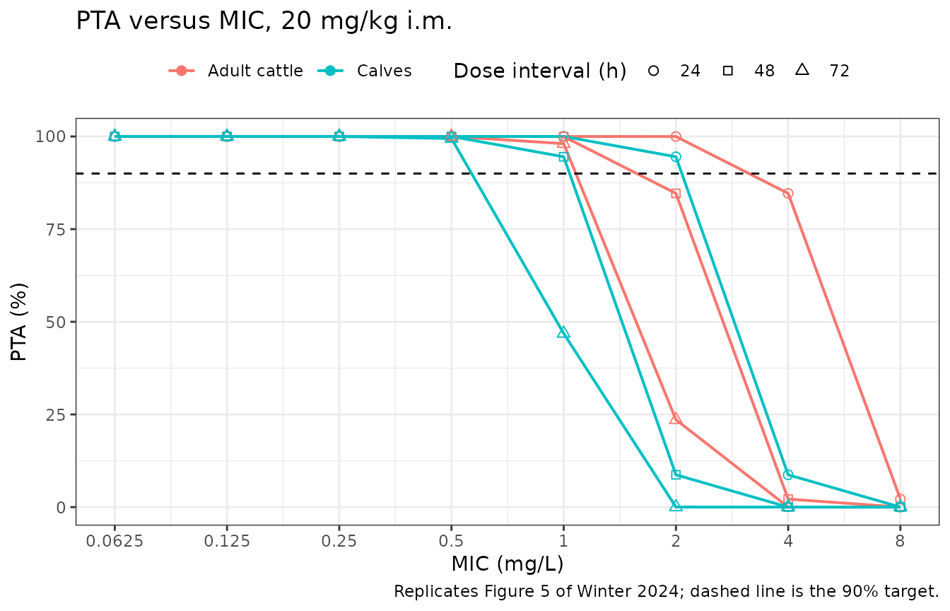
The ECOFF for Mannheimia haemolytica and Pasteurella multocida is 2 mg/L (Supplementary Table S5). The adult PK/PDCO of 2 mg/L at a 48 h interval meets it; the calf value of 1 mg/L does not, which is the paper’s central clinical finding.
Assumptions and deviations
-
Frapidis a plain fraction, not an ilogit-transformed one. Winter 2024 Table 1 lists the units of bothtvFrapidandtvF1as “ilogit”, and annotates thetvFrapidrow with “corresponding to a rapid F = 68.6%”, which isilogit(0.7828)- thetvFrapidvalue from the exploratorysource-covariate run in Supplementary Table S4, not the 0.757 printed in the same row. The Phoenix control stream in Supplementary Data S1 is unambiguous that only the total bioavailability is transformed:stparm(F1 = ilogit(tvF1 + nF1))versusstparm(Frapid = tvFrapid * exp(nFrapid)). Methods section 2.2.1.1 likewise introduces the transformation for “bioavailability (F)” alone, “to prevent the bioavailability being estimated greater than 100%”. The packaged model follows the control stream. This choice does not affect total exposure (AUC0-inf depends only onF1andCl) and therefore has no effect on any PK/PD cutoff above; it changes only the split between the fast and slow absorption phases. Checked against the supplementary raw data (404 observations from the 24 animals given a single 20 mg/kg i.m. dose and nothing else), the two readings fit comparably - median absolute log-residual against the typical-value prediction 0.24 for the control-stream reading and 0.21 for the “ilogit” reading - so the observed data do not discriminate them and the control stream is decisive. -
Frapidcan exceed 1 in the tails. BecauseFrapidcarries exponential IIV (BSV 12.7%) without a bound, about 1.4% of simulated animals drawffo > 1, which makesf(depot2)slightly negative. This is a property of the published parameterisation, not of the translation, and it is left in place. It does not produce negative concentrations at the cohort sizes used here (stopifnot(!anyNA(sim$Cc))above passes and no simulatedCcis negative), and it leaves total exposure exactly correct because the two depots still sum toF1 * Dose. -
Parameter values are the “Single run” estimates of Table
1, not the bootstrap medians in the adjacent columns and not
the
fixef()/ranef()numbers in Supplementary Data S1. The control-stream numbers are initial estimates carried over from the exploratorysource-covariate run - they match Supplementary Table S4, not Table 1 - so the control stream is used for structure only. -
The
sourcecovariate is not implemented. Winter 2024 explored a seven-level formulation/analytical-method covariate onKa2(Supplementary Table S4) but excluded it from the final model and deliberately from the Monte Carlo simulations, “so that the large variability in these simulations reflects the diversity of the EU formulations”. Sex, breed and health status were screened and rejected; they are recorded in the model’scovariatesDataExcludedmetadata. - Free fraction fixed at 50%. Winter 2024 section 2.2.2 sets plasma protein binding to 50% based on prior publications; reported estimates in cattle span 31.6-71.7%. The free fraction is a post-processing multiplier here, not a model parameter, so it appears only in the PK/PD sections of this vignette.
-
The Monte Carlo section uses a closed-form exposure
identity. The paper integrates
AUC0-1000h from the ODE system for 5,000 replicates. Because the terminal half-life is ~120 h, 1,000 h is effectively infinity andAUC0-1000h equalsF1 * Dose / Clto better than 0.01%; the cross-check table above confirms the closed-form and ODE-cohort 10th percentiles agree. The ODE cohort itself is capped at 200 animals per arm. - Small systematic under-prediction of the published cutoffs (~1-2%). The simulated PK/PDCO values are consistently a little below Table 4. Table 1 reports parameters to three or four significant figures, so the packaged values are slightly rounded relative to what the authors simulated with. No parameter has been tuned to close the gap.
-
Covariate naming. The paper’s
adult_calveindicator is carried under the canonical covariate columnCHILD(1 = calf, 0 = adult), whose register entry is the general juvenile-versus-adult age-cohort indicator. The species-specific cutoff (< 6 months) is documented in the model’scovariateData$CHILD$notes, as that register entry requires. -
Body-weight-normalised units. All parameters are
per kilogram, so
amtis a per-kilogram amount in ug/kg (a 20 mg/kg dose isamt = 20000) andCcis in ug/mL, equivalently mg/L. Simulating an absolute milligram dose without dividing by body weight would give concentrations wrong by the animal’s mass.