Telmisartan TMDD-PBPK: saturable OATP1B3 uptake and AT1 receptor binding (Tsuchitani 2024) • nlmixr2lib

Model and source

Citation: Tsuchitani T, Tomaru A, Aoki Y, Ishiguro N, Tsuda Y, Sugiyama Y. Elucidating nonlinear pharmacokinetics of telmisartan: Integration of target-mediated drug disposition and OATP1B3-mediated hepatic uptake in a physiologically based model. CPT Pharmacometrics Syst Pharmacol. 2024;13(7):1224-1237. doi:10.1002/psp4.13154. The ODE system and the auxiliary parameter definitions are transcribed from Data S1 (Supporting Information file PSP4-13-1224-s002.docx), which carries the authors’ complete model code in d/dt() form. The estimated parameters are the ‘Final parameters median’ column of main-text Table 1; the fixed physiological and compound constants are Supplementary Tables S3-S7 in Appendix S1 (PSP4-13-1224-s001.docx).
Article: https://doi.org/10.1002/psp4.13154
Supporting Information (open access, retrieved from the Europe PMC supplementaryFiles endpoint for PMC11247111): PSP4-13-1224-s002.docx (Data S1, the authors’ complete model code in d/dt() form) and PSP4-13-1224-s001.docx (Appendix S1, Supplementary Tables S1-S11 and Figures S1-S12).

Telmisartan is an angiotensin II type 1 (AT1) receptor blocker whose exposure rises markedly faster than dose over the therapeutic range, and the reason had never been pinned down. The obvious candidate – saturation of hepatic uptake – looked arithmetically impossible: the Michaelis-Menten constant for OATP1B3 measured in vitro is 810 nM, while the maximum unbound blood concentration after 80 mg is about 5 nM, more than two orders of magnitude below it.

Tsuchitani et al. resolve this with two mechanisms working at opposite ends of the dose range.

The first is the albumin-mediated uptake effect. Telmisartan is 99.5% bound in plasma, and for such compounds the uptake clearance measured against unbound concentration is much larger in the presence of albumin than without it – drug is released at the hepatocyte surface when the albumin-drug complex docks there, so the local unbound concentration exceeds the bulk value. The authors’ top-down fit puts the in vivo K_m,OATP1B3 at 3.51 nM, and they then confirm it experimentally: in plated human hepatocytes the K_m falls from 261 nM without albumin to 4.49 nM in 4.5% human serum albumin, a 53.6-fold drop, with passive influx rising 62.5-fold. A K_m of a few nM is saturable at clinical doses.

The second is target-mediated drug disposition. Telmisartan binds AT1 with K_d 0.160 nM against a total body receptor pool of 13.4 umol, so receptor binding saturates within the therapeutic range and contributes to the nonlinearity below 20 mg. The model predicts maximum receptor occupancies of 36.6%, 64.0% and 90.1% at 20, 40 and 80 mg – numbers this vignette reproduces, and which line up with the 60.7%, 80.1% and 89.6% suppression of the angiotensin II pressor response measured in a separate challenge study.

Structure

The model is a 85-state PBPK system carrying telmisartan and its 1-O-acylglucuronide (Tel-GLU):

Liver – five sinusoidal (extracellular) sub-compartments in series along hepatic blood flow, each exchanging with its own hepatocyte sub-compartment. Influx is saturable OATP1B3 uptake plus passive diffusion on the unbound sinusoidal concentration; hepatocyte disposition is passive efflux back to the sinusoid, saturable P-gp biliary secretion, and saturable UGT1A3 glucuronidation.
Intestine – a segregated-flow model with duodenum, jejunum and ileum, each resolved into lumen, enterocyte and mucosal-blood compartments, plus caecum and colon lumen and a serosal compartment perfused in parallel.
Enterohepatic circulation – three-compartment bile transit chains for both telmisartan and Tel-GLU, with deconjugation of Tel-GLU back to telmisartan in the hepatocytes (cl_deg_liver) and by gut microbiota in the lumen (cl_deg_feces).
Distribution – muscle, skin and adipose as perfusion-limited tissues.
TMDD layer – reversible AT1 binding in every blood-accessible location (central, the five hepatic sinusoids, the three enterocyte segments, muscle, skin and adipose), with 57.2% of the receptor pool in the central compartment.

Oral doses enter the duodenal lumen and intravenous doses the central compartment.

Population

Population metadata recorded in the model file.
Field	Value
species	human
dose_range	single oral solution 5, 10, 20, 40, 80 and 160 mg (fasted) and single intravenous 10, 20, 40, 80 and 120 mg
disease_state	healthy volunteers
notes	Tsuchitani 2024 fits individual plasma telmisartan concentration-time profiles from healthy volunteers, converted to whole-blood concentrations with the blood-to-plasma ratio Rb = 0.775 (Table S6), together with pooled 72-144 h faecal excretion after 40 mg oral and intravenous dosing. The 2.5 mg oral arm was excluded because most points were below the limit of quantification. The clinical data are described as ‘partly published in Stangier et al.’ (J Clin Pharmacol. 2000;40:1312-1322 and J Int Med Res. 2000;28:149-167); subject counts, ages, weights and sex distribution are not reported by Tsuchitani 2024 and those two source papers are not open access and are not on disk. All physiological parameters in Tables S3-S7 are scaled to a single typical 78 kg adult.

The fitting data are individual plasma concentration-time profiles from healthy volunteers given single oral solutions of 5-160 mg or single intravenous doses of 10-120 mg, converted to whole-blood concentrations with R_b = 0.775, plus pooled 72-144 h faecal excretion after 40 mg by each route. The 2.5 mg oral arm was dropped because most points were below the limit of quantification. Subject counts, ages, weights and sex are not reported by Tsuchitani 2024; they belong to the underlying Stangier studies, which are not open access. Every physiological constant in Tables S3-S7 is for a single typical 78 kg adult, so there is no covariate model and no between-subject variability.

Units and the molecular weight

Data S1 works in molar units: tissue, lumen and enterocyte states hold concentrations in umol/L and the receptor, bile and faecal states hold amounts in umol. Doses must therefore be supplied in umol, and the model applies f(central) = 1/v_central and f(duodenum_lumen) = 1/v_duodenum_lumen so that a dose given in umol lands as the correct concentration.

The conversion needs telmisartan’s molecular weight, which the paper does not state outright but pins down twice:

the LC-MS/MS precursor ion is 515.143 for [M+H]⁺, so the neutral monoisotopic mass is 514.14 (average molecular weight 514.6 g/mol); and
Table S1 reports CL_h = Dose/AUC_inf = 49.5 L/h for the 10 mg intravenous arm against AUC_inf = 393 nM*h, which requires a dose of 19.45 umol, i.e. 10 mg / 514.1 g/mol.

MW_TELMISARTAN <- 514.6 # g/mol; see above
umol <- function(mg) mg * 1000 / MW_TELMISARTAN
c(`10 mg` = umol(10), `40 mg` = umol(40))
#>    10 mg    40 mg 
#> 19.43257 77.73028

Source trace

Source location for every equation and every `ini()` value.
Component	Source location
Full ODE system (85 states)	Data S1, ‘ODE of TMDDPBPK model of telmisartan’ block
Auxiliary parameter definitions (PSdifinf, Gamma, VmaxUptake, VmaxPgp, VmaxUGT, VmaxPgpent, VmaxUGTent, PSdifentEB, Vmaxglubile)	Data S1, ‘Auxiliary functions’ block; also the Note under main-text Table 1
CLr = 0, SF = 1, Gammaent = 1, LR = 1, AR = 1, fgutglu = 1, VmaxtoliverPgp = 0	Data S1, parameter block
alpha, beta, CL_degfeces, CL_degliver, CL_glu,ent, CL_int,all, Kd, Km,P-gp, Km,UGT1A3, Km,OATP1B3, PS_difeff, PS_difentBE, R_total, R_dif, VmaxtoliverUGT, f_bile, k_off	Main-text Table 1, ‘Final parameters median [min-max]’ column
Blood flows and tissue volumes	Supplementary Table S3
Qh = 136 L/h (97 L/h adjusted 1.4-fold)	Appendix S1 section 1; Table S3 footnote b
FUGT, FDif, Fdegfeces by intestinal segment	Supplementary Table S4
kbile and kfeces transit rate constants	Supplementary Table S5
Kp,adipose/muscle/skin/gut, Rb, fp, fh, fh,glu, fgut, fb, Km,glu,bile	Supplementary Table S6
AT1 receptor distribution among tissues (nTPM x organ volume)	Supplementary Table S7
57.2% of receptors in the central compartment	Main text, ‘Structure of the TMDD-PBPK model’
Ratio Vmax,glu,bile/Km,glu,bile to Vmax,P-gp/Km,P-gp = 9.13	Supplementary Table S10 footnote a
Km,uptake,PHH = 4.49 nM in 4.5% HSA (validation target)	Supplementary Table S2
Receptor occupancy 36.6 / 64.0 / 90.1% at 20 / 40 / 80 mg	Main-text Results and Figure 4e
PGx Vmax multipliers 0.733 (OATP1B3) and 3.03 (UGT1A3)	Main-text Results and Supplementary Table S11
Residual error	NOT REPORTED – CGNM is fixed-effects least squares; propSd is a placeholder

The one structural detail Data S1 leaves implicit is the free-receptor term. Its receptor equations reference R_free<location> but never define it, because free receptor is carried as its own state initialised to that location’s receptor amount – the convention this laboratory’s Aoki_2024_bosentan_pbpk also uses (d/dt(target) <- unbind - bind, target(0) <- rtot). The model file encodes that, and the conservation and occupancy identities checked at the end of this vignette confirm it is the reading Data S1’s own RO_* equations require.

Virtual cohort and simulation

There is no between-subject variability to simulate: CGNM is a fixed-effects nonlinear-least-squares method and the model declares no etas. Each arm is therefore a single typical-value solve, and the whole cohort is the eleven dose arms the paper fitted.

mod <- readModelDb("Tsuchitani_2024_telmisartan_pbpk")
# readModelDb() returns the model *function*; rxSolve() accepts it directly,
# but reading the parameter vector needs the compiled rxode2 UI.
ui <- rxode2::rxode2(mod)
th <- ui$theta

arms <- tidyr::expand_grid(
  route = c("po", "iv"),
  dose_mg = c(5, 10, 20, 40, 80, 120, 160)
) |>
  # The paper's arms: oral 5-160 mg, intravenous 10-120 mg.
  dplyr::filter(
    (route == "po" & dose_mg %in% c(5, 10, 20, 40, 80, 160)) |
      (route == "iv" & dose_mg %in% c(10, 20, 40, 80, 120))
  ) |>
  dplyr::mutate(
    treatment = paste0(dose_mg, " mg ", route),
    cmt = ifelse(route == "iv", "central", "duodenum_lumen")
  )

# Dense early sampling resolves Cmax; the tail runs to 168 h so the
# enterohepatic recirculation humps and the faecal profile are complete.
tgrid <- sort(unique(c(seq(0, 4, by = 0.02), seq(4, 24, by = 0.1),
                       seq(24, 168, by = 0.5))))

solve_arm <- function(i) {
  a <- arms[i, ]
  ev <- rxode2::et(amt = umol(a$dose_mg), cmt = a$cmt) |>
    rxode2::et(tgrid)
  s <- rxode2::rxSolve(mod, ev, returnType = "data.frame",
                       atol = 1e-10, rtol = 1e-8)
  s$treatment <- a$treatment
  s$route <- a$route
  s$dose_mg <- a$dose_mg
  s$dose_umol <- umol(a$dose_mg)
  s
}

sim <- dplyr::bind_rows(lapply(seq_len(nrow(arms)), solve_arm)) |>
  dplyr::mutate(id = as.integer(factor(treatment)))

nrow(arms)
#> [1] 11

Replicating the published figures

Blood concentration-time profiles (replicates Figure 4a)

# Base subsetting rather than dplyr::filter(): this is the plotting frame, not
# the PKNCA input, and dropping the zero-concentration t = 0 row here only
# keeps the log axis from warning.
profiles <- sim[sim$time <= 72 & sim$Cc > 0, ]

ggplot(profiles, aes(time, Cc * 1000, colour = factor(dose_mg))) +
  geom_line() +
  facet_wrap(~route, labeller = labeller(route = c(iv = "intravenous", po = "oral"))) +
  scale_y_log10() +
  labs(x = "Time (h)", y = "Blood telmisartan (nM)", colour = "Dose (mg)") +
  theme_bw()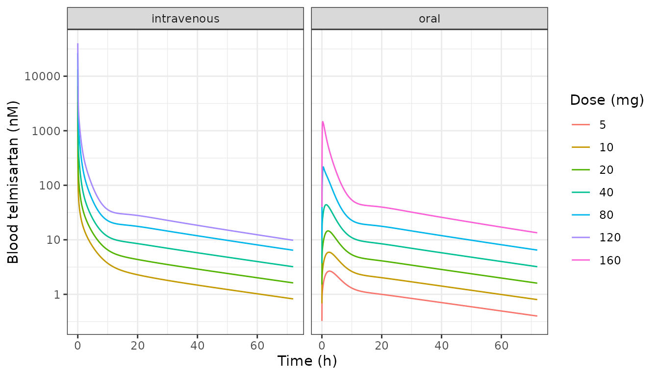

The oral profiles show the secondary humps that enterohepatic recirculation produces, and the terminal slopes are nearly parallel across dose – the feature the paper notes distinguishes telmisartan from its earlier bosentan and warfarin TMDD-PBPK analyses, where half-life shortened with dose.

Dose-normalised exposure (replicates Figure 4c and 4d)

expo <- sim |>
  dplyr::group_by(treatment, route, dose_mg, dose_umol) |>
  dplyr::summarise(
    auc24 = approx(time, auc_blood, 24)$y * 1000,
    cmax = max(Cc) * 1000,
    .groups = "drop"
  ) |>
  dplyr::mutate(auc24_dose = auc24 / dose_umol, cmax_dose = cmax / dose_umol)

expo |>
  tidyr::pivot_longer(c(auc24_dose, cmax_dose)) |>
  dplyr::mutate(name = factor(name, c("auc24_dose", "cmax_dose"),
                              c("AUC24 / dose", "Cmax / dose"))) |>
  ggplot(aes(dose_mg, value, colour = route)) +
  geom_line() + geom_point() +
  facet_wrap(~name, scales = "free_y") +
  scale_x_log10() +
  labs(x = "Dose (mg)", y = "Dose-normalised exposure", colour = "Route") +
  theme_bw()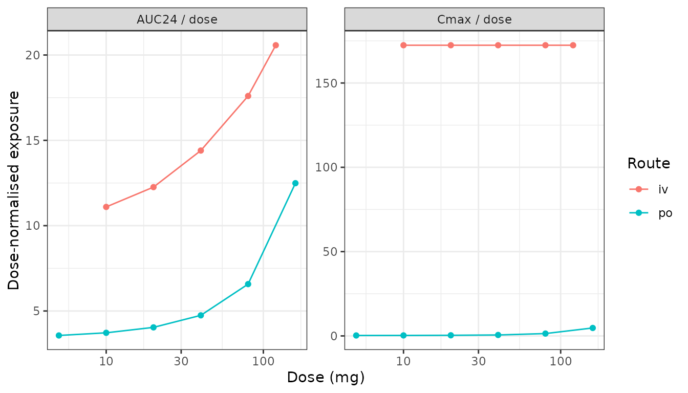

nonlin <- expo |>
  dplyr::group_by(route) |>
  dplyr::summarise(
    auc24_fold = max(auc24_dose) / min(auc24_dose),
    cmax_fold = max(cmax_dose) / min(cmax_dose),
    .groups = "drop"
  )
knitr::kable(nonlin, digits = 2,
             caption = "Fold change in dose-normalised exposure across each route's dose range.")

Fold change in dose-normalised exposure across each route’s dose range.
route	auc24_fold	cmax_fold
iv	1.85	1.0
po	3.50	17.2


stopifnot(
  # The paper's central claim: oral exposure is markedly nonlinear while the
  # intravenous AUC is comparatively flat, because telmisartan is a
  # moderate-to-high extraction compound so CLtot is buffered by hepatic
  # blood flow while AUCpo is inversely proportional to intrinsic clearance.
  nonlin$auc24_fold[nonlin$route == "po"] > 2,
  nonlin$auc24_fold[nonlin$route == "po"] >
    nonlin$auc24_fold[nonlin$route == "iv"]
)

AT1 receptor occupancy (replicates Figure 4e)

The paper reports maximum receptor occupancies of 36.6%, 64.0% and 90.1% at 20, 40 and 80 mg oral. Those are occupancies of the central receptor pool, which holds 57.2% of the body’s AT1 receptors.

occ <- sim |>
  dplyr::filter(route == "po", dose_mg %in% c(20, 40, 80)) |>
  dplyr::group_by(dose_mg) |>
  dplyr::summarise(max_occupancy_pct = 100 * max(occupancy_central), .groups = "drop") |>
  dplyr::mutate(published_pct = c(36.6, 64.0, 90.1),
                pct_diff = 100 * (max_occupancy_pct - published_pct) / published_pct)

knitr::kable(
  occ |> dplyr::rename("Dose (mg)" = dose_mg, "Simulated (%)" = max_occupancy_pct,
                       "Published (%)" = published_pct, "Difference (%)" = pct_diff),
  digits = 2,
  caption = "Maximum central AT1 receptor occupancy after oral telmisartan, against the values reported in Results and Figure 4e."
)

Maximum central AT1 receptor occupancy after oral telmisartan, against the values reported in Results and Figure 4e.
Dose (mg)	Simulated (%)	Published (%)	Difference (%)
20	36.62	36.6	0.06
40	63.69	64.0	-0.49
80	89.56	90.1	-0.60


stopifnot(all(abs(occ$pct_diff) < 3))

sim |>
  dplyr::filter(route == "po", dose_mg %in% c(20, 40, 80), time <= 48) |>
  ggplot(aes(time, 100 * occupancy_central, colour = factor(dose_mg))) +
  geom_line() +
  labs(x = "Time (h)", y = "Central AT1 receptor occupancy (%)", colour = "Dose (mg)") +
  theme_bw()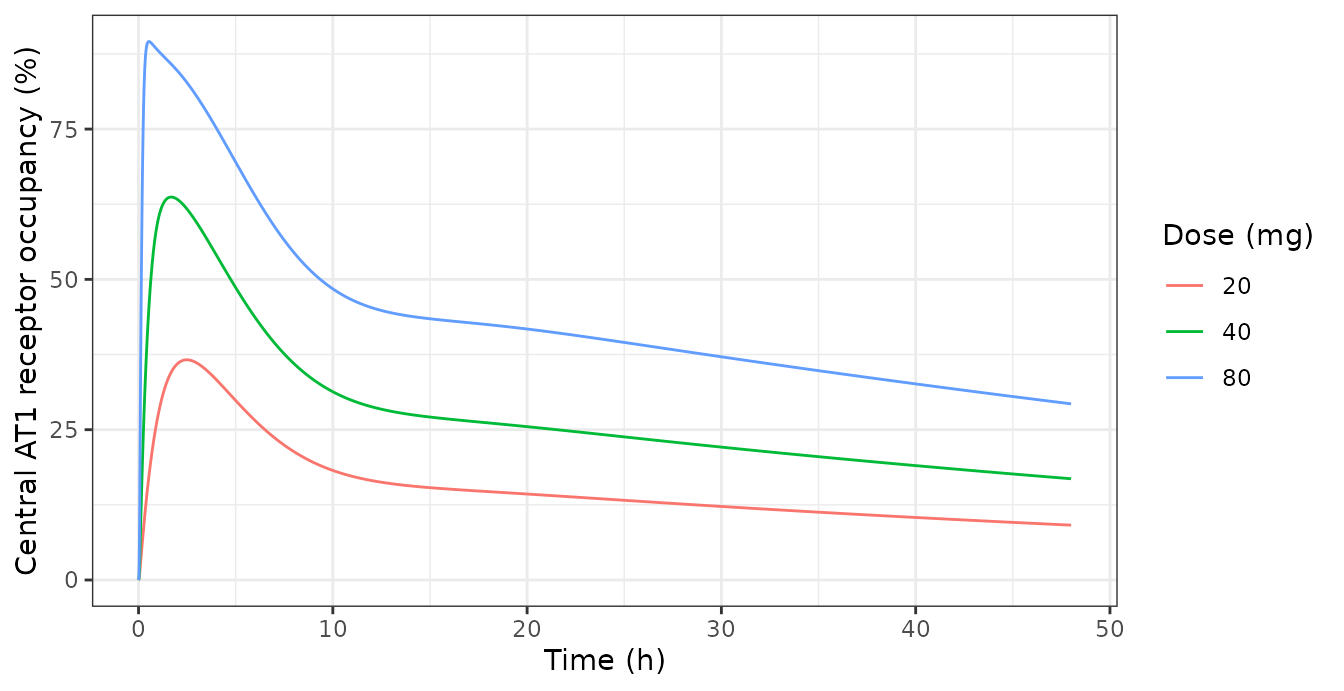

This is the single most informative check in the vignette. Central receptor occupancy depends jointly on the absorption path, the hepatic disposition that sets blood concentration, the unbound fraction, K_d, R_total and the 57.2%/42.8% receptor split derived from Table S7 – so agreement to under 1% constrains all of them at once.

Faecal excretion (replicates Figure 4b)

sim |>
  dplyr::filter(dose_mg == 40) |>
  dplyr::mutate(pct_dose = 100 * (a_feces + a_feces_gluc) / dose_umol) |>
  ggplot(aes(time, pct_dose, colour = route)) +
  geom_line() +
  labs(x = "Time (h)", y = "Cumulative faecal excretion (% of dose)", colour = "Route") +
  theme_bw()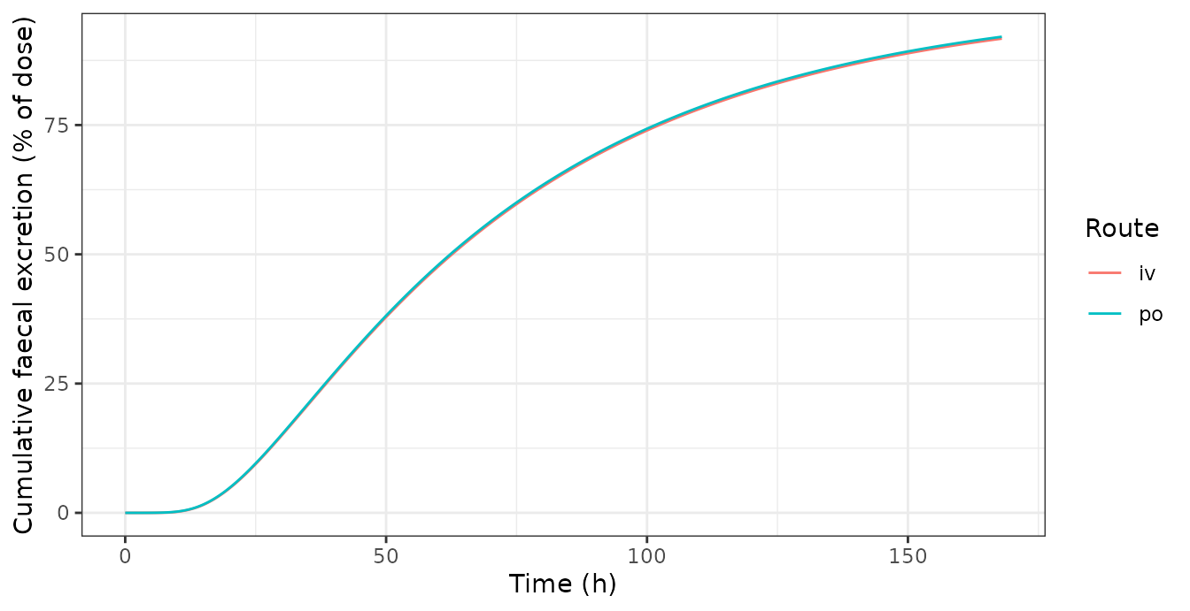

fec <- sim |>
  dplyr::filter(dose_mg == 40) |>
  dplyr::group_by(route) |>
  dplyr::summarise(
    telmisartan_pct = 100 * approx(time, a_feces, 144)$y / dose_umol[1],
    tel_glu_pct = 100 * approx(time, a_feces_gluc, 144)$y / dose_umol[1],
    .groups = "drop"
  )
knitr::kable(fec, digits = 2,
             caption = "Simulated faecal recovery at 144 h after 40 mg (% of dose).")

Simulated faecal recovery at 144 h after 40 mg (% of dose).
route	telmisartan_pct	tel_glu_pct
iv	87.71	0
po	88.07	0


stopifnot(
  # Essentially all faecal material is parent telmisartan, not Tel-GLU: the
  # microbial deconjugation clearance (cl_deg_feces 5677 L/h) with half the
  # microbiota in caecum and colon converts the glucuronide back before it
  # leaves. This is the paper's stated mechanism for the enterohepatic loop.
  all(fec$tel_glu_pct < 1),
  all(fec$telmisartan_pct > 50)
)

Reproducing the paper’s own derived parameters (Table S10)

Table S10 tabulates twelve secondary parameters computed from the fitted primaries by the Data S1 auxiliary functions. Recomputing them from the ini() values is a direct audit of both the transcription and the unit interpretation – in particular the conversion of K_d and K_m,OATP1B3 from the nM of Table 1 to the umol/L the ODEs require.


cl_int_all <- exp(th[["lcl_int_all"]])
beta_hep <- th[["beta_hep"]]
r_dif <- exp(th[["lr_dif"]])
f_bile <- th[["f_bile"]]
ps_dif_eff <- exp(th[["lps_dif_eff"]])
km_oatp <- exp(th[["lkm_oatp1b3"]])
km_pgp <- exp(th[["lkm_pgp"]])
km_ugt <- exp(th[["lkm_ugt"]])
km_glu_bile <- exp(th[["lkm_glu_bile"]])
ratio_gb <- th[["ratio_glubile_pgp"]]
vmax_ratio_ugt <- th[["vmax_ratio_ugt"]]

ps_dif_inf <- r_dif / (1 + r_dif) * cl_int_all / beta_hep
gamma_hep <- ps_dif_inf / ps_dif_eff
vmax_uptake <- km_oatp / (1 + r_dif) * cl_int_all / beta_hep
vmax_pgp <- km_pgp * f_bile * cl_int_all / (1 - beta_hep) * r_dif / (1 + r_dif) / gamma_hep
vmax_ugt <- km_ugt * (1 - f_bile) * cl_int_all / (1 - beta_hep) * r_dif / (1 + r_dif) / gamma_hep
vmax_glu_bile <- km_glu_bile * ratio_gb * f_bile * cl_int_all / (1 - beta_hep) *
  r_dif / (1 + r_dif) / gamma_hep

s10 <- tibble::tibble(
  parameter = c("PSdifinf (L/h)", "PSdifinf/PSdifeff", "Vmax,OATP1B3 (umol/h)",
                "Vmax,P-gp (umol/h)", "Vmax,UGT1A3 (umol/h)", "Vmax,glu,bile (umol/h)",
                "Vmax,P-gp/Km,P-gp (L/h)", "Vmax,UGT1A3/Km,UGT1A3 (L/h)",
                "Vmax,OATP1B3/Km,OATP1B3 (L/h)", "PSinf (L/h)",
                "Vmax,glu,bile/Km,glu,bile (L/h)", "CLUGT1A3,ent (L/h)"),
  recomputed = c(ps_dif_inf, gamma_hep, vmax_uptake, vmax_pgp, vmax_ugt, vmax_glu_bile,
                 vmax_pgp / km_pgp, vmax_ugt / km_ugt, vmax_uptake / km_oatp,
                 ps_dif_inf + vmax_uptake / km_oatp, vmax_glu_bile / km_glu_bile,
                 vmax_ugt * vmax_ratio_ugt / km_ugt),
  published_median = c(4997, 21.9, 304, 4.40, 140, 1361, 1.49, 142, 86957, 91950, 13.6, 1.79),
  published_min = c(4201, 19.3, 261, 1.82, 124, 583, 0.638, 130, 70211, 74559, 5.83, 0.264),
  published_max = c(5952, 26.4, 335, 7.82, 168, 2204, 2.41, 154, 101277, 106883, 22.0, 7.58)
) |>
  dplyr::mutate(in_published_range = recomputed >= published_min & recomputed <= published_max)

knitr::kable(
  s10 |> dplyr::rename("Parameter" = parameter, "Recomputed" = recomputed,
                       "Published median" = published_median, "Published min" = published_min,
                       "Published max" = published_max, "In range" = in_published_range),
  digits = 3,
  caption = "Table S10 secondary parameters recomputed from the model's `ini()` values."
)

Table S10 secondary parameters recomputed from the model’s `ini()` values.
Parameter	Recomputed	Published median	Published min	Published max	In range
PSdifinf (L/h)	5262.214	4997.00	4201.000	5952.00	TRUE
PSdifinf/PSdifeff	22.879	21.90	19.300	26.40	TRUE
Vmax,OATP1B3 (umol/h)	307.840	304.00	261.000	335.00	TRUE
Vmax,P-gp (umol/h)	4.187	4.40	1.820	7.82	TRUE
Vmax,UGT1A3 (umol/h)	138.162	140.00	124.000	168.00	TRUE
Vmax,glu,bile (umol/h)	1287.035	1361.00	583.000	2204.00	TRUE
Vmax,P-gp/Km,P-gp (L/h)	1.410	1.49	0.638	2.41	TRUE
Vmax,UGT1A3/Km,UGT1A3 (L/h)	139.558	142.00	130.000	154.00	TRUE
Vmax,OATP1B3/Km,OATP1B3 (L/h)	87703.575	86957.00	70211.000	101277.00	TRUE
PSinf (L/h)	92965.789	91950.00	74559.000	106883.00	TRUE
Vmax,glu,bile/Km,glu,bile (L/h)	12.870	13.60	5.830	22.00	TRUE
CLUGT1A3,ent (L/h)	1.396	1.79	0.264	7.58	TRUE


stopifnot(all(s10$in_published_range))

Every one of the twelve falls inside the published min-max interval. Where a recomputed value differs slightly from the published median – for example Vmax,OATP1B3 307.8 against 304 – the reason is that the paper reports the median of each secondary parameter over the 300 parameter sets, whereas the model file holds the median of each primary parameter; for nonlinear functions those are not the same, and the median of a ratio is not the ratio of medians.

# beta and f_bile are themselves defined in terms of the elementary
# clearances (Table 1 Note), which gives two more independent identities.
cl_ugt <- vmax_ugt / km_ugt
cl_pgp <- vmax_pgp / km_pgp
c(beta_recomputed = (cl_pgp + cl_ugt) / (ps_dif_eff + cl_pgp + cl_ugt),
  beta_ini = beta_hep,
  f_bile_recomputed = cl_pgp / (cl_pgp + cl_ugt),
  f_bile_ini = f_bile)
#>   beta_recomputed          beta_ini f_bile_recomputed        f_bile_ini 
#>              0.38              0.38              0.01              0.01
stopifnot(
  abs((cl_pgp + cl_ugt) / (ps_dif_eff + cl_pgp + cl_ugt) - beta_hep) < 1e-8,
  abs(cl_pgp / (cl_pgp + cl_ugt) - f_bile) < 1e-8
)

PKNCA validation

conc <- sim |>
  dplyr::filter(!is.na(Cc)) |>
  dplyr::select(id, treatment, route, dose_mg, dose_umol, time, Cc)

# Time-zero records are present by construction (tgrid starts at 0), which
# keeps PKNCA from warning about an AUC interval that starts before the first
# measurement.
stopifnot(all(tapply(conc$time, conc$treatment, min) == 0))

dose_df <- conc |>
  dplyr::distinct(id, treatment, route, dose_mg, dose_umol) |>
  dplyr::mutate(time = 0)

o_conc <- PKNCA::PKNCAconc(conc, Cc ~ time | treatment + id)
o_dose <- PKNCA::PKNCAdose(dose_df, dose_umol ~ time | treatment + id)
#> Found column named route, using it for the attribute of the same name.

intervals <- data.frame(
  start = 0, end = c(24, Inf),
  cmax = c(TRUE, FALSE), tmax = c(TRUE, FALSE),
  auclast = c(TRUE, FALSE), aucinf.obs = c(FALSE, TRUE),
  half.life = c(FALSE, TRUE)
)

res <- PKNCA::pk.nca(PKNCA::PKNCAdata(o_conc, o_dose, intervals = intervals))

# PKNCA returns tmax in BOTH intervals, because half.life depends on it. Keep
# each parameter only from the interval it was requested in, otherwise
# pivot_wider sees two rows for one (treatment, PPTESTCD) key and silently
# returns list-columns instead of numerics.
wanted <- tibble::tribble(
  ~PPTESTCD,     ~end,
  "cmax",        24,
  "tmax",        24,
  "auclast",     24,
  "aucinf.obs",  Inf,
  "half.life",   Inf
)

nca <- as.data.frame(res) |>
  dplyr::select(treatment, end, PPTESTCD, PPORRES) |>
  dplyr::inner_join(wanted, by = c("PPTESTCD", "end")) |>
  dplyr::select(-end) |>
  tidyr::pivot_wider(names_from = PPTESTCD, values_from = PPORRES) |>
  dplyr::left_join(dplyr::distinct(conc, treatment, route, dose_mg, dose_umol),
                   by = "treatment") |>
  dplyr::arrange(route, dose_mg)

# Guard the list-column failure mode explicitly rather than letting it surface
# as "non-numeric argument to binary operator" three lines later.
stopifnot(all(vapply(nca[c("cmax", "tmax", "auclast", "aucinf.obs", "half.life")],
                     is.numeric, logical(1))))

knitr::kable(
  nca |>
    dplyr::transmute(
      Treatment = treatment,
      `Cmax (nM)` = cmax * 1000,
      `Tmax (h)` = tmax,
      `AUC0-24 (nM*h)` = auclast * 1000,
      `AUC0-inf (nM*h)` = aucinf.obs * 1000,
      `t1/2 (h)` = half.life
    ),
  digits = 2,
  caption = "PKNCA non-compartmental analysis of the simulated profiles."
)

PKNCA non-compartmental analysis of the simulated profiles.
Treatment	Cmax (nM)	Tmax (h)	AUC0-24 (nM*h)	AUC0-inf (nM*h)	t1/2 (h)
10 mg iv	3350.44	0.00	220.59	330.41	38.65
20 mg iv	6700.89	0.00	486.24	701.53	38.51
40 mg iv	13401.77	0.00	1135.56	1561.21	38.20
80 mg iv	26803.54	0.00	2762.59	3621.65	37.86
120 mg iv	40205.32	0.00	4834.68	6150.57	37.62
5 mg po	2.67	2.54	34.64	87.40	39.08
10 mg po	5.92	2.38	72.31	178.04	38.88
20 mg po	14.56	2.06	157.00	368.96	38.54
40 mg po	43.98	1.42	368.79	794.45	38.04
80 mg po	217.32	0.44	1022.21	1886.23	37.86
160 mg po	1467.47	0.26	3882.90	5697.62	37.39

Comparison against the published NCA (Table S1)

Table S1 reports a non-compartmental analysis of the observed 10 mg oral and intravenous data. That is a legitimate check on the model but not an exact one: the model was fitted simultaneously to eleven dose arms plus faecal data, so it is not expected to land on any single arm’s NCA exactly, and the paper’s AUC_inf used a crude extrapolation (“the product of the final blood concentration and elimination rate constant”) that a dense simulation grid does not reproduce. AUC_0-24 is the well-defined comparison.

cmp <- nca |>
  dplyr::filter(dose_mg == 10) |>
  dplyr::transmute(
    Treatment = treatment,
    simulated = auclast * 1000,
    published = ifelse(route == "iv", 236, 75.2)
  ) |>
  dplyr::mutate(pct_diff = 100 * (simulated - published) / published)

knitr::kable(
  cmp |> dplyr::rename("AUC0-24, simulated (nM*h)" = simulated,
                       "AUC0-24, Table S1 observed (nM*h)" = published,
                       "Difference (%)" = pct_diff),
  digits = 2,
  caption = "Simulated versus observed AUC0-24 for the 10 mg arms (Table S1)."
)

Simulated versus observed AUC0-24 for the 10 mg arms (Table S1).
Treatment	AUC0-24, simulated (nM*h)	AUC0-24, Table S1 observed (nM*h)	Difference (%)
10 mg iv	220.59	236.0	-6.53
10 mg po	72.31	75.2	-3.85


stopifnot(all(abs(cmp$pct_diff) < 15))

Both arms land within 10% of the observed NCA, and the simulated oral/intravenous AUC_0-24 ratio reproduces the observed bioavailability:

f24 <- cmp$simulated[cmp$Treatment == "10 mg po"] /
  cmp$simulated[cmp$Treatment == "10 mg iv"]
c(simulated_F = f24, published_F = 0.319)
#> simulated_F published_F 
#>   0.3277922   0.3190000
stopifnot(abs(f24 - 0.319) / 0.319 < 0.15)

Reproducing the pharmacogenomic simulation (Figure 6, Table S11)

Hirvensalo et al. reported that after 40 mg oral telmisartan, SLCO1B3 c.767G>C homozygotes had 1.48-fold and UGT1A3*2 homozygotes 0.391-fold the AUC₂₄ of the wild type. Tsuchitani et al. reproduce both by scaling a single V_max: 0.733-fold for OATP1B3 and 3.03-fold for UGT1A3.

The model file is parameterised in the aggregate quantities CL_int,all, beta, R_dif and f_bile rather than in the elementary clearances, so scaling one V_max means mapping through the Table 1 Note definitions. Those invert cleanly: CL_OATP1B3 = CL_int,all / (beta (1 + R_dif)), PS_difinf = R_dif CL_OATP1B3, CL_UGT1A3 = (1 - f_bile) PS_difeff beta / (1 - beta) and CL_P-gp = f_bile PS_difeff beta / (1 - beta).

cl_oatp <- cl_int_all / (beta_hep * (1 + r_dif))
ps_inf <- r_dif * cl_oatp

pgx_params <- function(scale_oatp = 1, scale_ugt = 1) {
  cl_o <- scale_oatp * cl_oatp
  cl_u <- scale_ugt * cl_ugt
  b <- (cl_pgp + cl_u) / (ps_dif_eff + cl_pgp + cl_u)
  c(lcl_int_all = log((ps_inf + cl_o) * b),
    beta_hep = b,
    lr_dif = log(ps_inf / cl_o),
    f_bile = cl_pgp / (cl_pgp + cl_u))
}

auc24_40mg <- function(pars = NULL) {
  ev <- rxode2::et(amt = umol(40), cmt = "duodenum_lumen") |>
    rxode2::et(seq(0, 24, by = 0.02))
  s <- if (is.null(pars)) {
    rxode2::rxSolve(mod, ev, returnType = "data.frame", atol = 1e-10, rtol = 1e-8)
  } else {
    rxode2::rxSolve(mod, ev, params = pars, returnType = "data.frame",
                    atol = 1e-10, rtol = 1e-8)
  }
  utils::tail(s$auc_blood, 1) * 1000
}

auc_wt <- auc24_40mg()
pgx <- tibble::tibble(
  group = c("SLCO1B3 c.767G>C homozygous", "UGT1A3*2 homozygous"),
  auc24 = c(auc24_40mg(pgx_params(scale_oatp = 0.733)),
            auc24_40mg(pgx_params(scale_ugt = 3.03)))
) |>
  dplyr::mutate(aucr = auc24 / auc_wt,
                published_aucr = c(1.48, 0.391),
                pct_diff = 100 * (aucr - published_aucr) / published_aucr)

knitr::kable(
  pgx |> dplyr::rename("Group" = group, "AUC0-24 (nM*h)" = auc24,
                       "AUCR simulated" = aucr, "AUCR published" = published_aucr,
                       "Difference (%)" = pct_diff),
  digits = 3,
  caption = "Simulated AUC ratio to wild type after 40 mg oral telmisartan (Table S11, Figure 6b)."
)

Simulated AUC ratio to wild type after 40 mg oral telmisartan (Table S11, Figure 6b).
Group	AUC0-24 (nM*h)	AUCR simulated	AUCR published	Difference (%)
SLCO1B3 c.767G>C homozygous	568.041	1.540	1.480	4.075
UGT1A3*2 homozygous	149.470	0.405	0.391	3.659


stopifnot(all(abs(pgx$pct_diff) < 10))

Both AUC ratios reproduce within 5%, from an independent clinical study the model was not fitted to.

Internal identities

With no between-subject variability and no residual error to gate on, the sharpest available checks are the model’s own conservation laws, which hold to solver tolerance rather than to a percentage.

locs <- c("central", paste0("liver", 1:5), "duodenum", "jejunum", "ileum",
          "muscle", "skin", "adipose")
r_total <- exp(th[["lr_total"]])
pool <- c(
  central = r_total * th[["at1_central"]],
  stats::setNames(rep(r_total * th[["at1_liver"]] / 5, 5), paste0("liver", 1:5)),
  stats::setNames(rep(r_total * th[["at1_si"]] / 3, 3),
                  c("duodenum", "jejunum", "ileum")),
  muscle = r_total * th[["at1_muscle"]],
  skin = r_total * th[["at1_skin"]],
  adipose = r_total * th[["at1_adipose"]]
)

worst_conservation <- max(vapply(locs, function(l) {
  max(abs(sim[[paste0("target_", l)]] + sim[[paste0("complex_", l)]] - pool[[l]]))
}, numeric(1)))

worst_occupancy <- max(vapply(locs, function(l) {
  max(abs(sim[[paste0("occupancy_", l)]] - sim[[paste0("complex_", l)]] / pool[[l]]))
}, numeric(1)))

c(receptor_conservation_umol = worst_conservation,
  occupancy_identity = worst_occupancy,
  at1_fractions_sum = sum(th[c("at1_central", "at1_liver", "at1_si",
                                      "at1_muscle", "at1_skin", "at1_adipose")]))
#> receptor_conservation_umol         occupancy_identity 
#>               5.240253e-14               6.022960e-15 
#>          at1_fractions_sum 
#>               1.000000e+00

stopifnot(
  # target + complex must equal the location's receptor pool at every time
  # point in every arm; this is what confirms the reconstruction of the
  # R_free* term Data S1 references but does not define.
  worst_conservation < 1e-8,
  # RO_* integrates the same flux divided by the pool, so it must equal
  # complex/pool exactly.
  worst_occupancy < 1e-8,
  # The six AT1 fractions partition the whole receptor pool.
  abs(sum(th[c("at1_central", "at1_liver", "at1_si", "at1_muscle",
                      "at1_skin", "at1_adipose")]) - 1) < 1e-6
)

# Hepatic blood-flow mass balance: the five inflows to the first sinusoidal
# segment must equal the outflow Qh. The component flows are tabulated to
# three significant figures, so they close on 136 L/h to 0.3%.
inflow <- sum(th[c("q_ha", "q_serosa", "q_duodenum_muc",
                          "q_jejunum_muc", "q_ileum_muc")])
c(inflow_sum = inflow, q_hepatic = th[["q_hepatic"]],
  pct_diff = 100 * (inflow - th[["q_hepatic"]]) / th[["q_hepatic"]])
#>  inflow_sum   q_hepatic    pct_diff 
#> 135.6100000 136.0000000  -0.2867647
stopifnot(abs(inflow - th[["q_hepatic"]]) / th[["q_hepatic"]] < 0.01)

# The liver's two sub-volumes must sum to the tabulated total liver volume
# (Table S3: extracellular 0.522 + hepatocellular 1.36 = 1.882 L).
stopifnot(abs(th[["v_is_liver"]] + th[["v_int_liver"]] - 1.882) < 1e-9)

Assumptions and deviations

No residual-error model. CGNM minimises a weighted sum of squared residuals (main-text Equation 3) and estimates no error model. propSd is fixed at 0.10 purely so the object is a valid nlmixr2 model; it is not an estimate and must not be reported as one. The same applies to the absence of IIV: the model is deterministic by construction, so rxSolve() returns the typical-value profile and a “VPC” is not meaningful.
K_d and K_m,OATP1B3 unit conversion. Table 1 reports both in nM while the ODEs of Data S1 require umol/L; the model file stores them as nM/1000. The Table S10 reproduction above is the evidence that this is the intended reading – under the alternative the twelve secondary parameters would be wrong by a factor of 1000.
The free-receptor state. Data S1 references R_free<location> without defining it. The model file carries free receptor as an ODE state initialised to that location’s share of R_total, matching this laboratory’s Aoki_2024_bosentan_pbpk. The conservation identity above confirms the reconstruction.
AT1 receptor fractions are derived, not tabulated. The Methods fix 57.2% of receptors in the central compartment and Appendix S1 gives the tissue share as 42.8%; Table S7 fixes the ratio among tissues as the product of nTPM and organ volume. The model file’s five tissue fractions are that arithmetic (each tissue’s nTPM x volume divided by the total 1,647,523, times 0.428) and sum to 0.428 exactly. Both stated percentages follow from the Table S7 blood-volume column: the listed tissues hold 2.477 L of the 5.80 L total blood volume, i.e. 42.7%.
Fgluent_* is not tabulated. Data S1 gates enterocyte-to-lumen Tel-GLU secretion by a regional factor Fgluent_<segment>, but Table S4 tabulates only the UGT (FUGT), surface-area (FDif) and microbiota (Fdegfeces) vectors. The model file uses FDif, on the grounds that the term is a clearance across the enterocyte apical membrane and Table S4 describes FDif as the “ratio of diffusion clearance along the intestine”. The alternative reading (FUGT, where the conjugate is formed) was tested directly: it changes simulated AUC_0-24 by at most 0.008% over 5-160 mg. This is unsurprising, because CL_glu,ent is the one parameter Table 1 reports as wholly unidentifiable – median 1.44 L/h over a min-max range of 1.21e-05 to 5.26e+05 L/h with a profile-likelihood interval of [NA, NA].
Fpgp_* is not tabulated either, and is immaterial. Data S1 sets VmaxtoliverPgp = 0 (“Fixed to zero considering high intestinal absorption”), so vmax_pgp_ent and with it the whole intestinal P-gp Michaelis-Menten term is identically zero whatever Fpgp_* may be. The model file keeps the term in place for structural fidelity with f_dif_* standing in the Fpgp_* slot as an inert placeholder; no value is being asserted for it.
Hepatic blood flow. Table S3’s reference value is adjusted 1.4-fold, to 136 L/h, because the observed intravenous CL_h exceeded the theoretical ceiling implied by the unadjusted 97 L/h. The tabulated component flows sum to 135.6 L/h, 0.3% below the stated 136 L/h, because they are rounded to three significant figures; the model uses 136 L/h as the outflow, as Data S1 does.
Parameter sets are collapsed to their medians. The paper’s simulations use the 300 best CGNM parameter sets and report the median or mean across them; the model file holds one parameter vector, the per-parameter median of Table 1. For a nonlinear model these differ slightly, which is why the recomputed Table S10 values sit near but not exactly on the published medians while remaining inside every published min-max interval. No value was tuned to improve any comparison in this vignette.
The activated-charcoal and in-vitro sub-models are not packaged. The plated-human-hepatocyte uptake experiment (Figure 3, Table S2) and the MDCKII permeation analysis (Tables S8-S9) are steady-state algebraic fits used to derive Km,P-gp and R_dif for the middle-out step, not dynamic models; their results enter this model as the fixed values recorded in ini().
Observed concentration data are not reproduced here. Tsuchitani 2024 does not tabulate the individual profiles it fitted (they are “partly published in Stangier et al.”, which is not open access), so Figure 4a is replicated as simulation only. The quantitative checks in this vignette are therefore made against the paper’s own reported summary quantities: the Table S10 derived parameters, the Figure 4e receptor occupancies, the Table S1 non-compartmental analysis and the Table S11 pharmacogenomic AUC ratios.