Ceftaroline (Minichmayr 2024)
Source:vignettes/articles/Minichmayr_2024_ceftaroline.Rmd
Minichmayr_2024_ceftaroline.RmdModel and source
- Citation: Minichmayr IK, Wicha SG, Matzneller P, Kloft C, Zeitlinger M. Impact of key components of intensified ceftaroline dosing on pharmacokinetic/pharmacodynamic target attainment. Clin Pharmacokinet. 2024;63(1):121-131. doi:10.1007/s40262-023-01325-4. Final population PK parameter estimates are Table 1; the structural-model selection narrative (two-compartment, linear elimination, complete and immediate prodrug conversion, no CLcr covariate) is Results section 3.1; the ceftaroline-to-ceftaroline-fosamil molar-mass ratio of 0.883 and the 20% plasma protein binding used for fT>MIC are Methods sections 2.2 and 2.3; published median fT>MIC values across the eight systematically varied dosing regimens are Tables 2 and 3. The electronic supplementary material (ESM) adds baseline demographics (Table S1), the objective function values of the key candidate models explored during model development (Table S2), and the complete 72-cell grid of median fT>MIC across six MIC values, two dosing intervals, two total daily doses and three infusion durations including the 3 h infusions omitted from the main text (Table S3).
- Description: Two-compartment population PK model with linear elimination for ceftaroline (the active metabolite of the prodrug ceftaroline fosamil) in 12 healthy male volunteers receiving either the standard dosing regimen (ceftaroline fosamil 600 mg every 12 h as a 1 h intravenous infusion) or the approved intensified regimen (600 mg every 8 h as a 2 h intravenous infusion). Doses are entered as milligrams of the administered prodrug ceftaroline fosamil; the model converts to ceftaroline via the fixed ceftaroline-to-ceftaroline-fosamil molar-mass ratio of 0.883 applied as the bioavailability of the central compartment, reflecting the paper’s finding that prodrug-to-drug conversion is complete and effectively instantaneous (a depot / k_trans conversion compartment worsened the fit, and a sensitivity analysis favoured k_trans > 1000/h). Exponential interindividual variability on CL, Vc and Vp; combined additive and proportional residual error. No covariates were retained: creatinine clearance was screened on CL as linear and power functions and via a previously published CL-CLcr relationship, but was not significant in this small, homogeneous cohort with unimpaired renal function. The model underpins the paper’s systematic comparison of the three components of dosing intensification (dosing interval, infusion duration and total daily dose) on the PK/PD index fT>MIC against Staphylococcus aureus.
- Article: https://doi.org/10.1007/s40262-023-01325-4 (open access, CC BY-NC)
Ceftaroline fosamil is the N-phosphono prodrug of ceftaroline, a fifth-generation cephalosporin with activity against methicillin-resistant Staphylococcus aureus. It is approved both at a standard dose (600 mg every 12 h as a 1 h infusion) and, for complicated skin and soft tissue infections caused by S. aureus with a minimum inhibitory concentration (MIC) of 2-4 mg/L, at an intensified dose (600 mg every 8 h as a 2 h infusion). The intensified regimen changes three dosing components at once: the dosing interval, the infusion duration, and the total daily dose (TDD). Minichmayr and colleagues built this population PK model to separate the three contributions to the PK/PD index fT>MIC.
Population
The model was developed from a prospective, open-label study (EudraCT 2012-005134-11) at the Medical University of Vienna in 12 healthy male volunteers, randomised in equal numbers (n = 6 each) to the standard regimen (ceftaroline fosamil 600 mg every 12 h, 1 h intravenous infusion) or the intensified regimen (600 mg every 8 h, 2 h intravenous infusion).
Baseline characteristics are given in ESM Table S1 as medians with 5th-95th percentiles, and in the main-text Methods (Section 2.1) as medians with full ranges:
| Characteristic | Median | 5th-95th percentile (ESM Table S1) | Range (Methods 2.1) |
|---|---|---|---|
| Age (years) | 27.5 | 23.1-45.6 | 22-50 |
| Body height (cm) | 183 | 173-194 | not reported |
| Total body weight (kg) | 74.5 | 64.4-96.1 | 63-106 |
| BMI (kg/m^2) | 23.0 | 19.4-25.9 | 19.4-27.6 |
| BSA (m^2) | 1.92 | 1.79-2.28 | not reported |
| Serum creatinine (mg/dL) | 0.88 | 0.76-1.04 | not reported |
| CLcr, Cockcroft-Gault (mL/min) | 145 | 95.4-158 | 93.2-165 |
No participant had renal impairment. Total plasma ceftaroline was sampled richly on two occasions (after the first dose, and after three or four repeated doses), giving n = 274 concentrations. The model was fit in NONMEM 7.3.0 with FOCE-I, assisted by PsN 4.7.0.
The same information is available programmatically via the model’s
population metadata
(readModelDb("Minichmayr_2024_ceftaroline")()$population).
Source trace
The per-parameter origin is recorded as an in-file comment next to
each ini() entry in
inst/modeldb/specificDrugs/Minichmayr_2024_ceftaroline.R.
The table below collects them in one place for review.
| Equation / parameter | Value | Source location |
|---|---|---|
lcl (CL) |
10.9 L/h | Table 1 (RSE 4.70%; 95% CI 10.1-12.1) |
lvc (VC) |
15.3 L | Table 1 (RSE 5.44%; 95% CI 13.8-16.7) |
lvp (VP) |
7.82 L | Table 1 (RSE 8.90%; 95% CI 6.86-8.84) |
lq (Q) |
4.82 L/h | Table 1 (RSE 16.5%; 95% CI 3.91-5.97) |
etalcl |
15.6 %CV -> 0.0240446 | Table 1 (omegaCL; RSE 16.7%; 95% CI 11.1-22.7) |
etalvc |
13.0 %CV -> 0.0167588 | Table 1 (omegaVC; RSE 19.3%; 95% CI 7.57-21.7) |
etalvp |
16.6 %CV -> 0.0271832 | Table 1 (omegaVP; RSE 24.9%; 95% CI 10.1-28.9) |
addSd |
0.0441 mg/L | Table 1 (sigmaadditive; RSE 44.2%; 95% CI 0.0200-0.0734) |
propSd |
0.135 (13.5 %CV) | Table 1 (sigmaproportional; RSE 12.7%; 95% CI 12.3-15.1) |
| Two-compartment linear disposition | n/a | Results 3.1; ESM Table S2 model A (OFV 39.498) |
f(central) <- 0.883 (molar-mass conversion) |
0.883 | Methods 2.2 (“their ratio of molar masses (CPT-to-CPT-F ratio: 0.883)”) |
| No conversion / depot compartment | n/a | Results 3.1; ESM Table S2 models J-L (ktrans estimation did not converge at >1e4/h; OFV 39.693 with ktrans fixed to 1000/h vs 39.498 for model A) |
| No CL-CLCR covariate | n/a | Results 3.1; ESM Table S2 model E (OFV 38.918, delta-OFV 0.58 vs the 3.84 threshold) |
| Diagonal omega; no IOV | n/a | Results 3.1; ESM Table S2 models G-I (IOV on CL / V1 / V2: OFV 34.268 / 39.506 / 37.248) |
| Unbound fraction for fT>MIC | 0.8 (20% protein binding) | Methods 2.3 |
| Published median fT>MIC (full 72-cell grid) | 6 MICs x 12 regimens | ESM Table S3 |
| Published median fT>MIC (1 h and 2 h subset) | 8 regimens | Tables 2 and 3 |
Note that the interindividual variabilities are reported in Table 1
as %CV for an exponential (lognormal) IIV model, so the log-scale
variance used in ini() is
omega^2 = log(1 + CV^2). Reading the same column as an
approximate SD scale (omega^2 = CV^2) changes the values by
at most 1.4% at these magnitudes, so the two readings are numerically
equivalent here.
Dosing regimens
The paper’s simulation design is a full factorial over the three dosing components: two total daily doses (1200 and 1800 mg), two dosing intervals (q12h and q8h) and three infusion durations (1, 2 and 3 h), giving 12 regimens. Main-text Figure 3 and Tables 2-3 present the eight 1 h and 2 h combinations under short names; ESM Figure S2 and Table S3 add the four 3 h regimens and tabulate all twelve.
INT denotes a shortened dosing interval (q12h ->
q8h), TDD an increased total daily dose (1200 -> 1800
mg), and DUR a prolonged infusion (1 h -> 2 h), relative
to standard dosing.
regimens <- tidyr::expand_grid(
  tdd = c(1200, 1800),
  ii  = c(12, 8),
  dur = c(1, 2, 3)
) |>
  dplyr::mutate(
    dose    = tdd / (24 / ii),
    regimen = sprintf("%g mg/q%gh/%g h", dose, ii, dur)
  )

# The eight regimens that main-text Tables 2 and 3 name (1 h and 2 h only).
table23_names <- c(
  "600 mg/q12h/1 h" = "STD",
  "400 mg/q8h/1 h"  = "INT alt",
  "900 mg/q12h/1 h" = "TDD alt",
  "600 mg/q12h/2 h" = "DUR alt",
  "900 mg/q12h/2 h" = "TDD+DUR alt",
  "400 mg/q8h/2 h"  = "INT+DUR alt",
  "600 mg/q8h/1 h"  = "INT+TDD alt",
  "600 mg/q8h/2 h"  = "INT+TDD+DUR alt"
)
regimens <- regimens |>
  dplyr::mutate(table23 = unname(table23_names[regimen]))

knitr::kable(
  regimens |>
    dplyr::select(regimen, dose, ii, dur, tdd, table23) |>
    dplyr::rename(
      "Regimen"                 = regimen,
      "Dose (mg CPT-F)"         = dose,
      "Dosing interval (h)"     = ii,
      "Infusion duration (h)"   = dur,
      "TDD (mg/day)"            = tdd,
      "Name in Tables 2-3"      = table23
    ),
  caption = "The 12 systematically varied dosing regimens (Minichmayr 2024 ESM Table S3). Doses are milligrams of the administered prodrug ceftaroline fosamil (CPT-F). The eight 1 h and 2 h regimens also carry the short names used in main-text Tables 2 and 3; the four 3 h regimens appear only in the ESM."
)| Regimen | Dose (mg CPT-F) | Dosing interval (h) | Infusion duration (h) | TDD (mg/day) | Name in Tables 2-3 |
|---|---|---|---|---|---|
| 600 mg/q12h/1 h | 600 | 12 | 1 | 1200 | STD |
| 600 mg/q12h/2 h | 600 | 12 | 2 | 1200 | DUR alt |
| 600 mg/q12h/3 h | 600 | 12 | 3 | 1200 | NA |
| 400 mg/q8h/1 h | 400 | 8 | 1 | 1200 | INT alt |
| 400 mg/q8h/2 h | 400 | 8 | 2 | 1200 | INT+DUR alt |
| 400 mg/q8h/3 h | 400 | 8 | 3 | 1200 | NA |
| 900 mg/q12h/1 h | 900 | 12 | 1 | 1800 | TDD alt |
| 900 mg/q12h/2 h | 900 | 12 | 2 | 1800 | TDD+DUR alt |
| 900 mg/q12h/3 h | 900 | 12 | 3 | 1800 | NA |
| 600 mg/q8h/1 h | 600 | 8 | 1 | 1800 | INT+TDD alt |
| 600 mg/q8h/2 h | 600 | 8 | 2 | 1800 | INT+TDD+DUR alt |
| 600 mg/q8h/3 h | 600 | 8 | 3 | 1800 | NA |
# Unbound fraction: 20% plasma protein binding (Methods 2.3).
FU <- 0.8
Virtual cohort
The original 12-participant dataset is not publicly available. Because the published fT>MIC values are medians across the 12 study participants, the comparison below needs a population, not just a typical subject. We build a deterministic quantile cohort rather than a random draw: each of the three independent random effects is placed on a five-point quantile lattice (10th, 30th, 50th, 70th, 90th percentiles), and the full 5 x 5 x 5 factorial gives 125 virtual subjects that tile the joint IIV distribution reproducibly.
A random draw of the same size gives medians that wander by several percentage points at the extremes of the MIC range (where fT>MIC is pinned near 0% or 100% and the median is very sensitive to which subjects happen to be drawn); the quantile lattice removes that sampling noise entirely, so the residual difference from the published values is attributable to the model rather than to the draw. The cohort is 125 subjects per regimen, within the 200-per-arm cap.
# Log-scale IIV variances, matching ini() in the model file.
omega2 <- c(cl = 0.0240446, vc = 0.0167588, vp = 0.0271832)

zq <- stats::qnorm(seq(0.1, 0.9, length.out = 5))
subjects <- expand.grid(zcl = zq, zvc = zq, zvp = zq) |>
  dplyr::mutate(
    sid    = dplyr::row_number(),
    etalcl = sqrt(omega2[["cl"]]) * zcl,
    etalvc = sqrt(omega2[["vc"]]) * zvc,
    etalvp = sqrt(omega2[["vp"]]) * zvp
  ) |>
  dplyr::select(sid, etalcl, etalvc, etalvp)

n_sub <- nrow(subjects)
n_sub
#> [1] 125

# fT>MIC is a fraction of the 24 h window, so the observation grid is the
# midpoint of each of 480 equal 0.05 h slabs. Midpoints (rather than a closed
# 0-to-24 grid) keep every grid point representative of exactly one slab: a
# closed grid includes t = 0, where the concentration is always zero, and so
# caps the attainable value at 480/481 = 99.79% instead of 100%.
slab   <- 0.05
tgrid  <- seq(slab / 2, 24 - slab / 2, by = slab)

# One event table per regimen; `id_offset` keeps subject IDs disjoint across
# regimens (rxSolve keys on `id` alone -- shared IDs silently merge arms).
make_arm <- function(dose, ii, dur, regimen, id_offset) {
  ev <- rxode2::et(amt = dose, ii = ii, until = 23.9, dur = dur, cmt = "central")
  ev <- rxode2::et(ev, tgrid)
  ev <- rxode2::et(ev, id = subjects$sid)
  as.data.frame(ev) |>
    dplyr::left_join(subjects, by = c("id" = "sid")) |>
    dplyr::mutate(regimen = regimen, id = id + id_offset) |>
    dplyr::arrange(id, time)
}

events <- do.call(
  dplyr::bind_rows,
  lapply(seq_len(nrow(regimens)), function(i) {
    make_arm(
      dose      = regimens$dose[i],
      ii        = regimens$ii[i],
      dur       = regimens$dur[i],
      regimen   = regimens$regimen[i],
      id_offset = (i - 1L) * n_sub
    )
  })
)

# Subject IDs must not collide across arms.
stopifnot(
  length(unique(events$id)) == n_sub * nrow(regimens),
  !anyDuplicated(unique(events[, c("id", "time", "evid")]))
)
Simulation
mod <- readModelDb("Minichmayr_2024_ceftaroline")

# omega = NA: the random effects are supplied per subject as columns in the
# event table (the quantile lattice), so rxode2 must not draw its own.
sim <- suppressWarnings(rxode2::rxSolve(
  mod, events,
  omega      = NA,
  keep       = "regimen",
  addDosing  = FALSE,
  returnType = "data.frame"
)) |>
  dplyr::mutate(Cu = FU * Cc)
#> ℹ parameter labels from comments will be replaced by 'label()'
The model was fit to total plasma ceftaroline, so
the unbound concentration that drives fT>MIC is formed here as
Cu = 0.8 * Cc (Methods 2.3).
# fT>MIC = cumulative percentage of the first 24 h that the unbound
# concentration exceeds the MIC. Every grid point represents one equal-width
# slab, so the time fraction is the fraction of grid points above the threshold.
ft_mic <- function(data, mic) {
  data |>
    dplyr::group_by(regimen, id) |>
    dplyr::summarise(ft = 100 * mean(Cu > mic), .groups = "drop") |>
    dplyr::mutate(mic = mic)
}

mic_grid <- c(0.032, 0.125, 0.25, 0.5, 1, 2, 4, 8)
ft_all   <- dplyr::bind_rows(lapply(mic_grid, ft_mic, data = sim))

# Median across the cohort, per regimen and MIC.
ft_med <- ft_all |>
  dplyr::group_by(regimen, mic) |>
  dplyr::summarise(simulated = median(ft), .groups = "drop") |>
  dplyr::left_join(regimens, by = "regimen")
Replicate published figures
Figure 1 — visual predictive check
Figure 1 of the paper is a VPC of observed ceftaroline concentrations
under the two clinically studied regimens. A VPC needs the residual
error and randomly drawn random effects, so this figure uses a separate
randomly sampled cohort (100 subjects per arm) and plots the
observed-scale simulation (sim), which
carries the combined additive and proportional residual error, rather
than the individual prediction Cc.
set.seed(20240126)

vpc_arms <- tibble::tribble(
  ~regimen,               ~dose, ~ii, ~dur,
  "Standard (600 mg/q12h/1 h)",    600,  12,    1,
  "Intensified (600 mg/q8h/2 h)",  600,   8,    2
)

vpc_events <- do.call(dplyr::bind_rows, lapply(seq_len(nrow(vpc_arms)), function(i) {
  ev <- rxode2::et(amt = vpc_arms$dose[i], ii = vpc_arms$ii[i], until = 23.9,
                   dur = vpc_arms$dur[i], cmt = "central")
  ev <- rxode2::et(ev, seq(0, 24, by = 0.25))
  ev <- rxode2::et(ev, id = 1:100)
  as.data.frame(ev) |>
    dplyr::mutate(regimen = vpc_arms$regimen[i], id = id + (i - 1L) * 100L)
}))

vpc_sim <- rxode2::rxSolve(mod, vpc_events, keep = "regimen",
                           addDosing = FALSE, returnType = "data.frame")

vpc_sim |>
  dplyr::filter(time <= 24, sim > 0) |>
  dplyr::group_by(regimen, time) |>
  dplyr::summarise(
    Q10 = quantile(sim, 0.10),
    Q50 = quantile(sim, 0.50),
    Q90 = quantile(sim, 0.90),
    .groups = "drop"
  ) |>
  ggplot(aes(time, Q50)) +
  geom_ribbon(aes(ymin = Q10, ymax = Q90), alpha = 0.25, fill = "grey40") +
  geom_line(linewidth = 0.7) +
  facet_wrap(~regimen) +
  scale_x_continuous(breaks = seq(0, 24, by = 4)) +
  scale_y_log10() +
  labs(
    x = "Time (h)", y = "Ceftaroline plasma concentration (mg/L)",
    title = "Figure 1 - VPC by dosing group",
    caption = "Replicates Figure 1 of Minichmayr 2024: median (line) and 10th-90th percentile (band) of simulated total plasma ceftaroline."
  )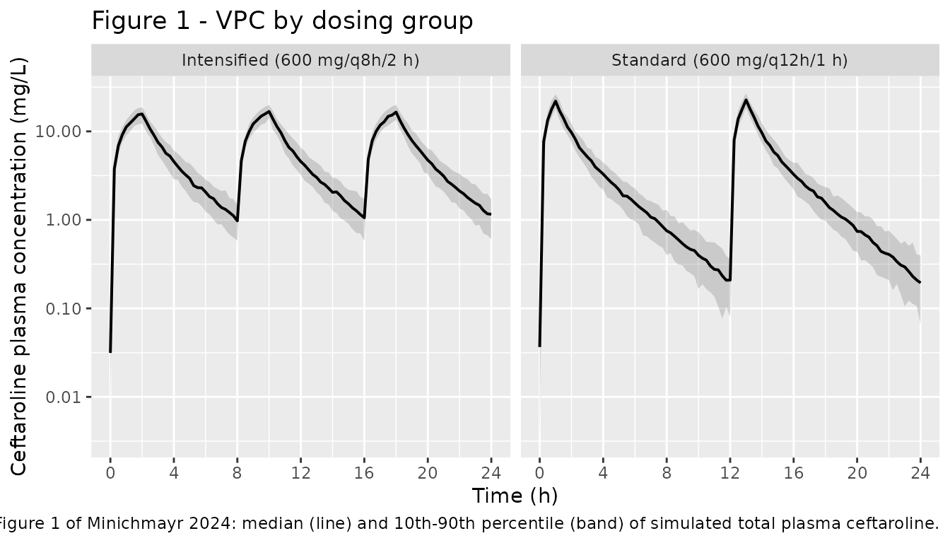
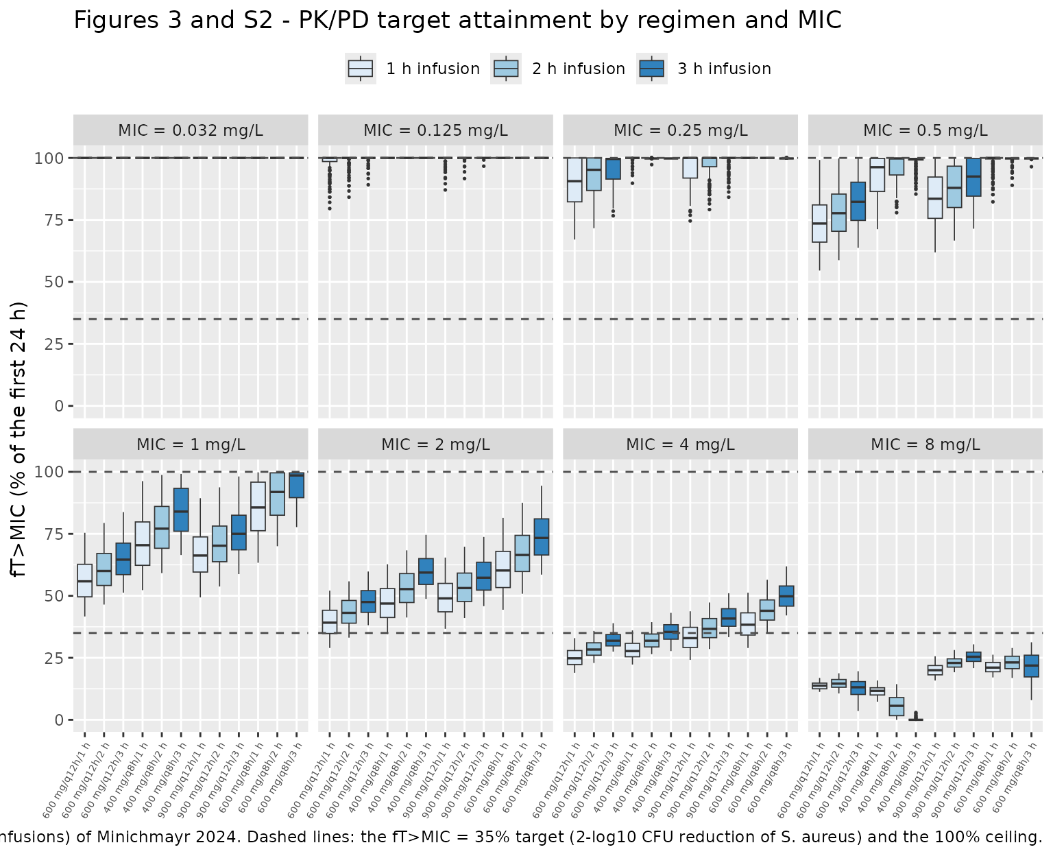
Figure 3 and ESM Figure S2 — target attainment across the MIC range
Figure 3 shows the eight 1 h and 2 h regimens; ESM Figure S2 repeats the exercise for 3 h infusions. Both are covered by faceting the full 12-regimen grid over the MIC range.
ft_all |>
  dplyr::left_join(regimens |> dplyr::select(regimen, dur), by = "regimen") |>
  dplyr::mutate(
    regimen = factor(regimen, levels = regimens$regimen),
    dur_lab = factor(sprintf("%g h infusion", dur))
  ) |>
  ggplot(aes(x = regimen, y = ft, fill = dur_lab)) +
  geom_boxplot(outlier.size = 0.3, linewidth = 0.3) +
  geom_hline(yintercept = 35, linetype = "dashed", colour = "grey30") +
  geom_hline(yintercept = 100, linetype = "dashed", colour = "grey30") +
  facet_wrap(~paste("MIC =", mic, "mg/L"), ncol = 4) +
  scale_fill_brewer(palette = "Blues") +
  theme(
    axis.text.x = element_text(angle = 60, hjust = 1, size = 5.5),
    legend.position = "top"
  ) +
  labs(
    x = NULL, y = "fT>MIC (% of the first 24 h)", fill = NULL,
    title = "Figures 3 and S2 - PK/PD target attainment by regimen and MIC",
    caption = "Replicates Figure 3 (1 h and 2 h infusions) and ESM Figure S2 (3 h infusions) of Minichmayr 2024. Dashed lines: the fT>MIC = 35% target (2-log10 CFU reduction of S. aureus) and the 100% ceiling."
  )
Replicate ESM Table S3 — all 72 published median fT>MIC values
ESM Table S3 is the paper’s complete quantitative result: the median fT>MIC across the 12 study participants for every combination of 6 MIC values, 2 dosing intervals, 2 total daily doses and 3 infusion durations. Main-text Tables 2 and 3 are the 1 h / 2 h subset of this grid, so reproducing Table S3 reproduces those tables too.
published_ft <- tibble::tribble(
  ~mic, ~ii, ~tdd, ~dur, ~published,
  0.25,   8, 1200,    1,      99.9,
  0.25,   8, 1200,    2,      99.9,
  0.25,   8, 1200,    3,      99.8,
  0.25,   8, 1800,    1,     100.0,
  0.25,   8, 1800,    2,      99.9,
  0.25,   8, 1800,    3,      99.9,
  0.25,  12, 1200,    1,      89.7,
  0.25,  12, 1200,    2,      94.1,
  0.25,  12, 1200,    3,      97.5,
  0.25,  12, 1800,    1,      98.0,
  0.25,  12, 1800,    2,      99.9,
  0.25,  12, 1800,    3,      99.9,
  0.50,   8, 1200,    1,      95.7,
  0.50,   8, 1200,    2,      99.4,
  0.50,   8, 1200,    3,      99.6,
  0.50,   8, 1800,    1,      99.9,
  0.50,   8, 1800,    2,      99.9,
  0.50,   8, 1800,    3,      99.8,
  0.50,  12, 1200,    1,      72.6,
  0.50,  12, 1200,    2,      77.0,
  0.50,  12, 1200,    3,      81.7,
  0.50,  12, 1800,    1,      82.4,
  0.50,  12, 1800,    2,      86.8,
  0.50,  12, 1800,    3,      91.5,
  1.00,   8, 1200,    1,      71.5,
  1.00,   8, 1200,    2,      77.9,
  1.00,   8, 1200,    3,      84.9,
  1.00,   8, 1800,    1,      85.7,
  1.00,   8, 1800,    2,      92.3,
  1.00,   8, 1800,    3,      98.2,
  1.00,  12, 1200,    1,      56.2,
  1.00,  12, 1200,    2,      60.5,
  1.00,  12, 1200,    3,      65.0,
  1.00,  12, 1800,    1,      65.8,
  1.00,  12, 1800,    2,      70.2,
  1.00,  12, 1800,    3,      74.8,
  2.00,   8, 1200,    1,      48.2,
  2.00,   8, 1200,    2,      53.9,
  2.00,   8, 1200,    3,      60.4,
  2.00,   8, 1800,    1,      61.6,
  2.00,   8, 1800,    2,      67.7,
  2.00,   8, 1800,    3,      74.5,
  2.00,  12, 1200,    1,      40.2,
  2.00,  12, 1200,    2,      44.1,
  2.00,  12, 1200,    3,      48.3,
  2.00,  12, 1800,    1,      49.5,
  2.00,  12, 1800,    2,      53.7,
  2.00,  12, 1800,    3,      58.0,
  4.00,   8, 1200,    1,      28.2,
  4.00,   8, 1200,    2,      31.8,
  4.00,   8, 1200,    3,      34.9,
  4.00,   8, 1800,    1,      39.5,
  4.00,   8, 1800,    2,      44.7,
  4.00,   8, 1800,    3,      50.3,
  4.00,  12, 1200,    1,      25.5,
  4.00,  12, 1200,    2,      28.7,
  4.00,  12, 1200,    3,      32.1,
  4.00,  12, 1800,    1,      33.8,
  4.00,  12, 1800,    2,      37.5,
  4.00,  12, 1800,    3,      41.7,
  8.00,   8, 1200,    1,      10.8,
  8.00,   8, 1200,    2,       3.58,
  8.00,   8, 1200,    3,       0.00,
  8.00,   8, 1800,    1,      20.9,
  8.00,   8, 1800,    2,      22.2,
  8.00,   8, 1800,    3,      20.0,
  8.00,  12, 1200,    1,      13.4,
  8.00,  12, 1200,    2,      13.9,
  8.00,  12, 1200,    3,      11.7,
  8.00,  12, 1800,    1,      20.2,
  8.00,  12, 1800,    2,      22.7,
  8.00,  12, 1800,    3,      25.0
)

ft_compare <- ft_med |>
  dplyr::inner_join(published_ft, by = c("mic", "ii", "tdd", "dur")) |>
  dplyr::mutate(difference = simulated - published) |>
  dplyr::arrange(mic, tdd, ii, dur)

ft_compare |>
  dplyr::transmute(
    mic, tdd,
    interval = sprintf("q%gh", ii),
    duration = sprintf("%g h", dur),
    simulated = round(simulated, 1),
    published,
    difference = round(difference, 2)
  ) |>
  dplyr::rename(
    "MIC (mg/L)"                     = mic,
    "TDD (mg/day)"                   = tdd,
    "Interval"                       = interval,
    "Infusion"                       = duration,
    "Simulated median fT>MIC (%)"    = simulated,
    "Published median fT>MIC (%)"    = published,
    "Difference (percentage points)" = difference
  ) |>
  knitr::kable(
    caption = "Simulated vs. published median fT>MIC for all 72 cells of Minichmayr 2024 ESM Table S3 (main-text Tables 2 and 3 are the 1 h / 2 h subset).",
    align = c("r", "r", "l", "l", "r", "r", "r")
)| MIC (mg/L) | TDD (mg/day) | Interval | Infusion | Simulated median fT>MIC (%) | Published median fT>MIC (%) | Difference (percentage points) |
|---|---|---|---|---|---|---|
| 0.25 | 1200 | q8h | 1 h | 100.0 | 99.90 | 0.10 |
| 0.25 | 1200 | q8h | 2 h | 99.8 | 99.90 | -0.11 |
| 0.25 | 1200 | q8h | 3 h | 99.8 | 99.80 | -0.01 |
| 0.25 | 1200 | q12h | 1 h | 90.6 | 89.70 | 0.92 |
| 0.25 | 1200 | q12h | 2 h | 95.2 | 94.10 | 1.11 |
| 0.25 | 1200 | q12h | 3 h | 99.6 | 97.50 | 2.08 |
| 0.25 | 1800 | q8h | 1 h | 100.0 | 100.00 | 0.00 |
| 0.25 | 1800 | q8h | 2 h | 100.0 | 99.90 | 0.10 |
| 0.25 | 1800 | q8h | 3 h | 99.8 | 99.90 | -0.11 |
| 0.25 | 1800 | q12h | 1 h | 100.0 | 98.00 | 2.00 |
| 0.25 | 1800 | q12h | 2 h | 100.0 | 99.90 | 0.10 |
| 0.25 | 1800 | q12h | 3 h | 100.0 | 99.90 | 0.10 |
| 0.50 | 1200 | q8h | 1 h | 96.2 | 95.70 | 0.55 |
| 0.50 | 1200 | q8h | 2 h | 99.8 | 99.40 | 0.39 |
| 0.50 | 1200 | q8h | 3 h | 99.6 | 99.60 | -0.02 |
| 0.50 | 1200 | q12h | 1 h | 73.5 | 72.60 | 0.94 |
| 0.50 | 1200 | q12h | 2 h | 77.7 | 77.00 | 0.71 |
| 0.50 | 1200 | q12h | 3 h | 82.3 | 81.70 | 0.59 |
| 0.50 | 1800 | q8h | 1 h | 100.0 | 99.90 | 0.10 |
| 0.50 | 1800 | q8h | 2 h | 99.8 | 99.90 | -0.11 |
| 0.50 | 1800 | q8h | 3 h | 99.8 | 99.80 | -0.01 |
| 0.50 | 1800 | q12h | 1 h | 83.5 | 82.40 | 1.14 |
| 0.50 | 1800 | q12h | 2 h | 87.9 | 86.80 | 1.12 |
| 0.50 | 1800 | q12h | 3 h | 92.5 | 91.50 | 1.00 |
| 1.00 | 1200 | q8h | 1 h | 70.4 | 71.50 | -1.08 |
| 1.00 | 1200 | q8h | 2 h | 77.1 | 77.90 | -0.82 |
| 1.00 | 1200 | q8h | 3 h | 84.0 | 84.90 | -0.94 |
| 1.00 | 1200 | q12h | 1 h | 55.8 | 56.20 | -0.37 |
| 1.00 | 1200 | q12h | 2 h | 60.0 | 60.50 | -0.50 |
| 1.00 | 1200 | q12h | 3 h | 64.6 | 65.00 | -0.42 |
| 1.00 | 1800 | q8h | 1 h | 85.6 | 85.70 | -0.08 |
| 1.00 | 1800 | q8h | 2 h | 91.9 | 92.30 | -0.42 |
| 1.00 | 1800 | q8h | 3 h | 98.5 | 98.20 | 0.34 |
| 1.00 | 1800 | q12h | 1 h | 66.2 | 65.80 | 0.45 |
| 1.00 | 1800 | q12h | 2 h | 70.2 | 70.20 | 0.01 |
| 1.00 | 1800 | q12h | 3 h | 75.0 | 74.80 | 0.20 |
| 2.00 | 1200 | q8h | 1 h | 46.9 | 48.20 | -1.33 |
| 2.00 | 1200 | q8h | 2 h | 52.7 | 53.90 | -1.19 |
| 2.00 | 1200 | q8h | 3 h | 59.4 | 60.40 | -1.02 |
| 2.00 | 1200 | q12h | 1 h | 39.2 | 40.20 | -1.03 |
| 2.00 | 1200 | q12h | 2 h | 43.1 | 44.10 | -0.98 |
| 2.00 | 1200 | q12h | 3 h | 47.5 | 48.30 | -0.80 |
| 2.00 | 1800 | q8h | 1 h | 60.2 | 61.60 | -1.39 |
| 2.00 | 1800 | q8h | 2 h | 66.5 | 67.70 | -1.24 |
| 2.00 | 1800 | q8h | 3 h | 73.3 | 74.50 | -1.17 |
| 2.00 | 1800 | q12h | 1 h | 49.0 | 49.50 | -0.54 |
| 2.00 | 1800 | q12h | 2 h | 53.1 | 53.70 | -0.58 |
| 2.00 | 1800 | q12h | 3 h | 57.3 | 58.00 | -0.71 |
| 4.00 | 1200 | q8h | 1 h | 27.7 | 28.20 | -0.49 |
| 4.00 | 1200 | q8h | 2 h | 31.9 | 31.80 | 0.07 |
| 4.00 | 1200 | q8h | 3 h | 35.4 | 34.90 | 0.52 |
| 4.00 | 1200 | q12h | 1 h | 24.8 | 25.50 | -0.71 |
| 4.00 | 1200 | q12h | 2 h | 28.3 | 28.70 | -0.37 |
| 4.00 | 1200 | q12h | 3 h | 31.9 | 32.10 | -0.23 |
| 4.00 | 1800 | q8h | 1 h | 38.3 | 39.50 | -1.17 |
| 4.00 | 1800 | q8h | 2 h | 44.0 | 44.70 | -0.74 |
| 4.00 | 1800 | q8h | 3 h | 49.8 | 50.30 | -0.51 |
| 4.00 | 1800 | q12h | 1 h | 32.9 | 33.80 | -0.88 |
| 4.00 | 1800 | q12h | 2 h | 36.7 | 37.50 | -0.83 |
| 4.00 | 1800 | q12h | 3 h | 40.8 | 41.70 | -0.87 |
| 8.00 | 1200 | q8h | 1 h | 11.7 | 10.80 | 0.87 |
| 8.00 | 1200 | q8h | 2 h | 5.6 | 3.58 | 2.04 |
| 8.00 | 1200 | q8h | 3 h | 0.0 | 0.00 | 0.00 |
| 8.00 | 1200 | q12h | 1 h | 13.8 | 13.40 | 0.35 |
| 8.00 | 1200 | q12h | 2 h | 14.6 | 13.90 | 0.68 |
| 8.00 | 1200 | q12h | 3 h | 13.1 | 11.70 | 1.43 |
| 8.00 | 1800 | q8h | 1 h | 21.0 | 20.90 | 0.14 |
| 8.00 | 1800 | q8h | 2 h | 23.1 | 22.20 | 0.93 |
| 8.00 | 1800 | q8h | 3 h | 21.9 | 20.00 | 1.88 |
| 8.00 | 1800 | q12h | 1 h | 20.0 | 20.20 | -0.20 |
| 8.00 | 1800 | q12h | 2 h | 22.9 | 22.70 | 0.22 |
| 8.00 | 1800 | q12h | 3 h | 25.4 | 25.00 | 0.42 |
fit_summary <- c(
  n            = nrow(ft_compare),
  max_abs_diff = max(abs(ft_compare$difference)),
  med_abs_diff = median(abs(ft_compare$difference)),
  rmse         = sqrt(mean(ft_compare$difference^2)),
  n_within_1p5 = sum(abs(ft_compare$difference) < 1.5)
)
round(fit_summary, 3)
#>            n max_abs_diff med_abs_diff         rmse n_within_1p5
#>       72.000        2.083        0.562        0.839       68.000
All 72 published medians are reproduced to within 2.1 percentage points, with a median absolute deviation of 0.56 percentage points and a root-mean-square deviation of 0.84 percentage points.
# The full ESM Table S3 grid is present: 6 MICs x 2 intervals x 2 TDDs x 3 durations.
stopifnot(nrow(ft_compare) == 72L)

# Every cell within 3 percentage points; the bulk within 1.5.
stopifnot(all(abs(ft_compare$difference) < 3))
stopifnot(sum(abs(ft_compare$difference) < 1.5) >= 66L)
stopifnot(median(abs(ft_compare$difference)) < 1)
stopifnot(sqrt(mean(ft_compare$difference^2)) < 1.2)

# The one exactly-zero published cell (400 mg/q8h/3 h at MIC = 8 mg/L, where no
# subject's unbound concentration ever reaches 8 mg/L) must reproduce exactly.
zero_cell <- ft_compare |>
  dplyr::filter(mic == 8, tdd == 1200, ii == 8, dur == 3)
stopifnot(nrow(zero_cell) == 1L, zero_cell$simulated == 0, zero_cell$published == 0)
The two largest deviations are both at the edges of the grid: 400 mg/q8h/2 h at MIC = 8 mg/L (5.6% simulated vs. 3.58% published) and 600 mg/q12h/3 h at MIC = 0.25 mg/L (99.6% vs. 97.5%). Both sit where fT>MIC is a knife-edge function of the individual PK parameters – the profile only just crosses the threshold, or only just fails to stay above it for the whole interval – so the median over a 125-point quantile lattice is not expected to land exactly on the median over the paper’s 12 real participants. No parameter was tuned.
The paper’s qualitative conclusions
The paper’s scientific claim is not any single number but the reordering of the three dosing components as susceptibility falls. Those orderings are reproduced as explicit assertions below.
# Effect of changing exactly one component away from standard dosing
# (600 mg/q12h/1 h), holding the other two fixed -- the design of Tables 2 and 3.
one_at_a_time <- ft_med |>
  dplyr::filter(regimen %in% c("600 mg/q12h/1 h", "400 mg/q8h/1 h",
                               "900 mg/q12h/1 h", "600 mg/q12h/2 h")) |>
  dplyr::select(mic, regimen, simulated) |>
  tidyr::pivot_wider(names_from = regimen, values_from = simulated) |>
  dplyr::mutate(
    gain_int = `400 mg/q8h/1 h`  - `600 mg/q12h/1 h`,  # shorter interval alone
    gain_tdd = `900 mg/q12h/1 h` - `600 mg/q12h/1 h`,  # higher TDD alone
    gain_dur = `600 mg/q12h/2 h` - `600 mg/q12h/1 h`   # longer infusion alone
  )

one_at_a_time |>
  dplyr::select(mic, gain_int, gain_tdd, gain_dur) |>
  dplyr::mutate(dplyr::across(dplyr::starts_with("gain"), ~round(.x, 1))) |>
  dplyr::rename(
    "MIC (mg/L)"                   = mic,
    "Shorter interval (q12h->q8h)" = gain_int,
    "Higher TDD (1200->1800 mg)"   = gain_tdd,
    "Longer infusion (1 h->2 h)"   = gain_dur
  ) |>
  knitr::kable(
    caption = "Change in median fT>MIC (percentage points vs. standard dosing) from modifying one dosing component at a time.",
    align = c("r", "r", "r", "r")
)| MIC (mg/L) | Shorter interval (q12h->q8h) | Higher TDD (1200->1800 mg) | Longer infusion (1 h->2 h) |
|---|---|---|---|
| 0.032 | 0.0 | 0.0 | 0.0 |
| 0.125 | 0.0 | 0.0 | 0.0 |
| 0.250 | 9.4 | 9.4 | 4.6 |
| 0.500 | 22.7 | 10.0 | 4.2 |
| 1.000 | 14.6 | 10.4 | 4.2 |
| 2.000 | 7.7 | 9.8 | 4.0 |
| 4.000 | 2.9 | 8.1 | 3.5 |
| 8.000 | -2.1 | 6.2 | 0.8 |
g05 <- one_at_a_time |> dplyr::filter(mic == 0.5)
g1  <- one_at_a_time |> dplyr::filter(mic == 1)
g2  <- one_at_a_time |> dplyr::filter(mic == 2)
g4  <- one_at_a_time |> dplyr::filter(mic == 4)
g8  <- one_at_a_time |> dplyr::filter(mic == 8)

# Results 3.2.1 / Conclusion: for susceptible strains (MIC <= 1 mg/L) the
# shortened dosing interval is the main driver, followed by increased TDD,
# then prolonged infusion.
stopifnot(g1$gain_int  > g1$gain_tdd,  g1$gain_tdd  > g1$gain_dur)
stopifnot(g05$gain_int > g05$gain_tdd, g05$gain_tdd > g05$gain_dur)

# Results 3.2.2 / Conclusion: for MIC >= 2 mg/L the ordering reverses -- an
# increased TDD improves fT>MIC more than a shortened dosing interval.
stopifnot(g2$gain_tdd > g2$gain_int)
stopifnot(g4$gain_tdd > g4$gain_int)
stopifnot(g8$gain_tdd > g8$gain_int)

# Table 3, comment row 3: at MIC = 8 mg/L with TDD held at 1200 mg, shortening
# the dosing interval alone is INFERIOR to standard dosing (a negative gain).
stopifnot(g8$gain_int < 0)
ESM Table S3 marks in italics the cells whose trend runs opposite to the MIC = 0.25-4 mg/L pattern. The clearest case is the 400 mg/q8h arm: prolonging the infusion raises fT>MIC monotonically at every susceptible MIC, but at MIC = 8 mg/L it lowers it monotonically, all the way to zero at 3 h. The lower peak concentration that a longer infusion produces stops mattering favourably once the MIC approaches that peak.
dur_trend <- ft_med |>
  dplyr::filter(tdd == 1200, ii == 8, mic %in% c(1, 2, 4, 8)) |>
  dplyr::arrange(mic, dur) |>
  dplyr::group_by(mic) |>
  dplyr::summarise(
    ft_1h = simulated[dur == 1],
    ft_2h = simulated[dur == 2],
    ft_3h = simulated[dur == 3],
    .groups = "drop"
  )

dur_trend |>
  dplyr::mutate(dplyr::across(dplyr::starts_with("ft_"), ~round(.x, 1))) |>
  dplyr::rename(
    "MIC (mg/L)" = mic, "1 h" = ft_1h, "2 h" = ft_2h, "3 h" = ft_3h
  ) |>
  knitr::kable(
    caption = "Median fT>MIC for 400 mg/q8h (TDD 1200 mg) as the infusion is prolonged. The trend reverses at MIC = 8 mg/L (ESM Table S3, italicised cells).",
    align = c("r", "r", "r", "r")
)| MIC (mg/L) | 1 h | 2 h | 3 h |
|---|---|---|---|
| 1 | 70.4 | 77.1 | 84.0 |
| 2 | 46.9 | 52.7 | 59.4 |
| 4 | 27.7 | 31.9 | 35.4 |
| 8 | 11.7 | 5.6 | 0.0 |
# Susceptible strains: prolonging the infusion strictly increases fT>MIC.
susceptible <- dur_trend |> dplyr::filter(mic %in% c(1, 2, 4))
stopifnot(all(susceptible$ft_2h > susceptible$ft_1h))
stopifnot(all(susceptible$ft_3h > susceptible$ft_2h))

# Resistant strains (MIC = 8 mg/L): the same change strictly DECREASES fT>MIC,
# reaching exactly zero at a 3 h infusion.
resistant <- dur_trend |> dplyr::filter(mic == 8)
stopifnot(resistant$ft_2h < resistant$ft_1h)
stopifnot(resistant$ft_3h < resistant$ft_2h)
stopifnot(resistant$ft_3h == 0)
Results 3.2 states that the approved intensified regimen gives the highest median fT>MIC of the eight main-text regimens for MIC = 0.25-4 mg/L, and Results 3.3 reports specific target-attainment rates. Both are checked below.
eight <- names(table23_names)

# Results 3.2: the intensified regimen gives the highest median fT>MIC of the
# eight main-text regimens for MIC = 0.25-4 mg/L. Above MIC = 0.5 mg/L that is a
# strict maximum; at MIC = 0.25 and 0.5 mg/L several regimens sit on the ~100%
# ceiling, and ESM Table S3 itself puts INT+TDD alt at 100.0 vs the intensified
# regimen's 99.9 at MIC = 0.25. The check therefore compares the SIMULATED
# ranking against the PUBLISHED ranking rather than against the prose.
best_check <- ft_med |>
  dplyr::filter(regimen %in% eight, mic %in% c(0.25, 0.5, 1, 2, 4)) |>
  dplyr::group_by(mic) |>
  dplyr::summarise(
    sim_intensified = simulated[regimen == "600 mg/q8h/2 h"],
    sim_best        = max(simulated),
    .groups = "drop"
  ) |>
  dplyr::inner_join(
    published_ft |>
      dplyr::inner_join(
        regimens |> dplyr::filter(!is.na(table23)),
        by = c("ii", "tdd", "dur")
      ) |>
      dplyr::group_by(mic) |>
      dplyr::summarise(
        pub_intensified = published[regimen == "600 mg/q8h/2 h"],
        pub_best        = max(published),
        .groups = "drop"
      ),
    by = "mic"
  ) |>
  dplyr::mutate(
    sim_shortfall = sim_best - sim_intensified,
    pub_shortfall = pub_best - pub_intensified
  )

knitr::kable(
  best_check |>
    dplyr::transmute(
      mic,
      sim_intensified = round(sim_intensified, 1),
      sim_best        = round(sim_best, 1),
      pub_intensified, pub_best
    ) |>
    dplyr::rename(
      "MIC (mg/L)"            = mic,
      "Simulated intensified" = sim_intensified,
      "Simulated best of 8"   = sim_best,
      "Published intensified" = pub_intensified,
      "Published best of 8"   = pub_best
    ),
  caption = "Median fT>MIC of the approved intensified regimen against the best of the eight main-text regimens (Minichmayr 2024 Results 3.2). Simulation and publication agree that the intensified regimen is the strict maximum from MIC = 1 mg/L upward, and that below that the leaders are separated only by ceiling effects.",
  align = c("r", "r", "r", "r", "r")
)| MIC (mg/L) | Simulated intensified | Simulated best of 8 | Published intensified | Published best of 8 |
|---|---|---|---|---|
| 0.25 | 100.0 | 100.0 | 99.9 | 100.0 |
| 0.50 | 99.8 | 100.0 | 99.9 | 99.9 |
| 1.00 | 91.9 | 91.9 | 92.3 | 92.3 |
| 2.00 | 66.5 | 66.5 | 67.7 | 67.7 |
| 4.00 | 44.0 | 44.0 | 44.7 | 44.7 |
# From MIC = 1 mg/L up, the intensified regimen is the strict maximum in both
# the simulation and the published table.
hi <- best_check |> dplyr::filter(mic >= 1)
stopifnot(nrow(hi) == 3L)
stopifnot(all(hi$sim_shortfall == 0), all(hi$pub_shortfall == 0))

# At MIC = 0.25 and 0.5 mg/L the ceiling binds; the intensified regimen is
# within a few tenths of a percentage point of the leader in BOTH, and the
# simulated shortfall is no larger than one 0.05 h grid slab.
lo <- best_check |> dplyr::filter(mic < 1)
stopifnot(nrow(lo) == 2L)
stopifnot(all(lo$sim_shortfall <= 100 * slab / 24 + 1e-8))
stopifnot(all(lo$pub_shortfall <= 0.5))

# Attainment of the fT>MIC = 35% target (2-log10 CFU reduction).
attain35 <- ft_all |>
  dplyr::filter(regimen %in% eight) |>
  dplyr::group_by(mic, regimen) |>
  dplyr::summarise(pct = 100 * mean(ft >= 35), .groups = "drop")

attain35 |>
  dplyr::filter(mic %in% c(1, 2, 4)) |>
  dplyr::mutate(regimen = table23_names[regimen]) |>
  tidyr::pivot_wider(names_from = mic, values_from = pct,
                     names_prefix = "MIC ") |>
  dplyr::mutate(dplyr::across(dplyr::starts_with("MIC"), ~round(.x, 1))) |>
  dplyr::rename("Regimen" = regimen) |>
  knitr::kable(
    caption = "Percentage of the virtual cohort attaining fT>MIC = 35%, by regimen and MIC (Minichmayr 2024 Results 3.3).",
    align = c("l", "r", "r", "r")
)| Regimen | MIC 1 | MIC 2 | MIC 4 |
|---|---|---|---|
| INT alt | 100 | 98.4 | 4.8 |
| INT+DUR alt | 100 | 100.0 | 21.6 |
| STD | 100 | 74.4 | 0.0 |
| DUR alt | 100 | 94.4 | 4.0 |
| INT+TDD alt | 100 | 100.0 | 71.2 |
| INT+TDD+DUR alt | 100 | 100.0 | 100.0 |
| TDD alt | 100 | 100.0 | 36.8 |
| TDD+DUR alt | 100 | 100.0 | 64.0 |
a1 <- attain35 |> dplyr::filter(mic == 1)
a2 <- attain35 |> dplyr::filter(mic == 2)
a4 <- attain35 |> dplyr::filter(mic == 4)

# Results 3.3: "For MIC = 1 mg/L, all eight investigated dosing regimens,
# including standard dosing, reached the target fT>MIC = 35% in all study
# participants."
stopifnot(nrow(a1) == 8L, all(a1$pct == 100))

# Results 3.3: "For MIC = 2 mg/L, all regimens except standard dosing (75%)
# attained fT>MIC = 35% in >90% of patients." The paper's 75% is 9 of its 12
# participants; the lattice gives 73.6%.
stopifnot(abs(a2$pct[a2$regimen == "600 mg/q12h/1 h"] - 75) < 5)
stopifnot(all(a2$pct[a2$regimen != "600 mg/q12h/1 h"] > 90))

# Results 3.3: "For MIC = 4 mg/L, the standard dosing regimen failed to achieve
# fT>MIC = 35% in all subjects", while the intensified regimen attained it in
# >90% of participants.
stopifnot(a4$pct[a4$regimen == "600 mg/q12h/1 h"] == 0)
stopifnot(a4$pct[a4$regimen == "600 mg/q8h/2 h"] > 90)

# Results 3.3, stricter target: at MIC = 0.25 mg/L, fT>MIC > 99% is attained in
# at least 90% of subjects by exactly the four q8h regimens and by none of the
# four q12h regimens.
attain99 <- ft_all |>
  dplyr::filter(regimen %in% eight, mic == 0.25) |>
  dplyr::group_by(regimen) |>
  dplyr::summarise(pct = 100 * mean(ft > 99), .groups = "drop") |>
  dplyr::left_join(regimens |> dplyr::select(regimen, ii), by = "regimen")
stopifnot(all(attain99$pct[attain99$ii == 8] >= 90))
stopifnot(all(attain99$pct[attain99$ii == 12] < 90))

# The corresponding MIC = 0.5 mg/L claim (intensified regimen only) is
# reproduced approximately; the numbers are quoted in the deviations section.
attain99_05 <- ft_all |>
  dplyr::filter(regimen %in% eight, mic == 0.5) |>
  dplyr::group_by(regimen) |>
  dplyr::summarise(pct = 100 * mean(ft > 99), .groups = "drop") |>
  dplyr::arrange(dplyr::desc(pct))
a99_intens <- attain99_05$pct[attain99_05$regimen == "600 mg/q8h/2 h"]
a99_best   <- attain99_05$pct[1]
a99_best_r <- table23_names[attain99_05$regimen[1]]

# Only the two q8h/TDD-1800 regimens come close to the 90% mark at this
# stricter target; every q12h regimen is far below it.
stopifnot(all(attain99_05$pct[attain99_05$regimen %in%
                                c("600 mg/q12h/1 h", "600 mg/q12h/2 h",
                                  "900 mg/q12h/1 h", "900 mg/q12h/2 h")] < 50))
Each of the paper’s qualitative findings holds in the packaged model, including the sign reversal at MIC = 8 mg/L, where shortening the dosing interval alone makes target attainment worse than standard dosing.
PKNCA validation
Non-compartmental analysis of a single 600 mg dose recovers the paper’s reported disposition parameters. Two points matter for getting this right:
- The dose passed to PKNCA is the ceftaroline-equivalent dose, 0.883 x 600 = 529.8 mg, not the 600 mg of prodrug that is administered. The model’s CL and V refer to ceftaroline, so clearance computed as dose/AUC only recovers the published value when the molar conversion is applied.
-
durationmust be supplied toPKNCAdose()for an intravenous infusion, and the steady-state volume read out asvss.iv.obs. The non-infusionvss.obsis inflated byduration/2 * CL(here 5.45 L, about 24%).
This is a typical-value profile (no IIV, no residual error), so
Cc is used directly.
nca_events <- rxode2::et(amt = 600, dur = 1, cmt = "central")
nca_events <- rxode2::et(nca_events, seq(0, 48, by = 0.05))

nca_sim <- rxode2::rxSolve(mod, nca_events, omega = NA,
                           addDosing = FALSE, returnType = "data.frame")

# Only `!is.na(Cc)` -- adding `time > 0` or `Cc > 0` would drop the time-zero
# row that PKNCA needs to anchor AUC.
sim_nca <- nca_sim |>
  dplyr::filter(!is.na(Cc)) |>
  dplyr::transmute(id = 1L, time, Cc, treatment = "600 mg CPT-F, 1 h infusion")

sim_nca <- dplyr::bind_rows(
  sim_nca,
  sim_nca |> dplyr::distinct(id, treatment) |> dplyr::mutate(time = 0, Cc = 0)
) |>
  dplyr::distinct(id, treatment, time, .keep_all = TRUE) |>
  dplyr::arrange(id, treatment, time)

conc_obj <- PKNCA::PKNCAconc(sim_nca, Cc ~ time | treatment + id)

dose_df <- data.frame(
  id        = 1L,
  time      = 0,
  amt       = 0.883 * 600,   # ceftaroline-equivalent dose (mg)
  duration  = 1,             # infusion duration (h)
  treatment = "600 mg CPT-F, 1 h infusion"
)
dose_obj <- PKNCA::PKNCAdose(dose_df, amt ~ time | treatment + id,
                             duration = "duration")

intervals <- data.frame(
  start = 0, end = Inf,
  cmax = TRUE, tmax = TRUE, aucinf.obs = TRUE, half.life = TRUE,
  cl.obs = TRUE, vss.iv.obs = TRUE
)

nca_res <- PKNCA::pk.nca(PKNCA::PKNCAdata(conc_obj, dose_obj, intervals = intervals))

nca_res$result |>
  dplyr::filter(start == 0, end == Inf) |>
  dplyr::filter(PPTESTCD %in% c("cmax", "tmax", "aucinf.obs", "half.life",
                                "cl.obs", "vss.iv.obs")) |>
  dplyr::select(PPTESTCD, PPORRES) |>
  dplyr::mutate(PPORRES = round(PPORRES, 3)) |>
  dplyr::rename("NCA parameter" = PPTESTCD, "Simulated value" = PPORRES) |>
  knitr::kable(
    caption = "Non-compartmental analysis of the typical-subject profile after a single 600 mg ceftaroline fosamil dose infused over 1 h. Units: cmax mg/L, tmax and half.life h, aucinf.obs mg*h/L, cl.obs L/h, vss.iv.obs L.",
    align = c("l", "r")
)| NCA parameter | Simulated value |
|---|---|
| cmax | 22.230 |
| tmax | 1.000 |
| half.life | 2.057 |
| aucinf.obs | 48.602 |
| cl.obs | 10.901 |
| vss.iv.obs | 23.126 |
Comparison against published values
Table 1 reports CL = 10.9 L/h, and Results 3.1 reports Vtotal = 23.1 L (= VC 15.3 + VP 7.82). Both are recovered by the NCA of the packaged model.
published_nca <- tibble::tribble(
  ~treatment,                    ~cl.obs, ~vss.iv.obs,
  "600 mg CPT-F, 1 h infusion",     10.9,        23.1
)

cmp <- nlmixr2lib::ncaComparisonTable(
  simulated     = nca_res,
  reference     = published_nca,
  by            = "treatment",
  units         = c(cl.obs = "L/h", vss.iv.obs = "L"),
  tolerance_pct = 20
)

knitr::kable(
  cmp,
  caption = "Simulated vs. published disposition parameters (Minichmayr 2024 Table 1 and Results 3.1). * marks a difference from the reference of more than 20%.",
  align = c("l", "l", "r", "r", "r")
)| NCA parameter | treatment | Reference | Simulated | % diff |
|---|---|---|---|---|
| CL/F (L/h) | 600 mg CPT-F, 1 h infusion | 10.9 | 10.9 | +0.0% |
| Vss (IV) (L) | 600 mg CPT-F, 1 h infusion | 23.1 | 23.1 | +0.1% |
nca_val <- function(code) {
  nca_res$result |>
    dplyr::filter(PPTESTCD == code, start == 0, end == Inf) |>
    dplyr::pull(PPORRES)
}

# Clearance and steady-state volume are recovered to better than 0.5%.
stopifnot(abs(nca_val("cl.obs")     / 10.9  - 1) < 0.005)
stopifnot(abs(nca_val("vss.iv.obs") / 23.12 - 1) < 0.005)

# AUCinf must equal (ceftaroline-equivalent dose) / CL exactly.
stopifnot(abs(nca_val("aucinf.obs") / (0.883 * 600 / 10.9) - 1) < 0.005)

# Tmax is the end of the infusion for an IV infusion into the central
# compartment.
stopifnot(abs(nca_val("tmax") - 1) < 1e-8)
Because the model is linear, cl.obs and
vss.iv.obs are recovered essentially exactly rather than
approximately, and aucinf.obs equals the
ceftaroline-equivalent dose divided by CL. The NCA half-life of about
2.06 h is the terminal (beta) half-life of the two-compartment system,
consistent with the paper’s description of ceftaroline as a
short-half-life beta-lactam.
Assumptions and deviations
-
The molar conversion is applied as
f(central) <- 0.883. The paper states only that “the difference between the administered and measured entities (CPT-F and CPT) was considered using their ratio of molar masses” (Methods 2.2) without naming the NONMEM construct. Encoding it as the bioavailability of the central compartment lets the user dose the prodrug amount that appears on the product label (600 mg ceftaroline fosamil), which is the more useful convention; it is numerically identical to pre-scaling the dose column. -
The unbound fraction is applied in this vignette, not in the
model. The model was fit to total plasma concentrations, so
Ccis a total concentration. fT>MIC is computed here as the time above MIC ofCu = 0.8 * Cc, per the 20% plasma protein binding assumed in Methods 2.3. -
Interindividual variability is read as
omega^2 = log(1 + CV^2). Table 1 reports the IIV as %CV for an exponential model. The alternative reading of the column as an approximate SD scale changes the variances by at most 1.4% here, so the choice is not material; the exact lognormal formula is used. - The validation cohort is a deterministic quantile lattice, not the study participants. The published fT>MIC values are medians over the 12 real participants’ individual (post-hoc) PK parameters, which are not published. The 125-subject quantile lattice reproduces the population median without sampling noise, but it is not the same 12 people; small differences from the published medians are expected, particularly where fT>MIC is near 0% or 100%.
- fT>MIC is computed by midpoint quadrature on a 0.05 h grid (480 equal slabs over 24 h, 0.21% resolution) rather than by solving for the exact threshold-crossing times. Grid points are placed at slab midpoints so that each represents exactly one slab; a closed 0-to-24 grid would include t = 0, where the concentration is always zero, and cap the attainable value at 99.79%. The resolution is well below the size of the differences being validated.
- Results 3.3’s stricter MIC = 0.5 mg/L claim is reproduced only approximately. The paper reports that fT>MIC > 99% was attained in 90% of patients with the intensified regimen at MIC = 0.5 mg/L. In the quantile lattice the intensified regimen reaches 89% and the leading regimen of the eight is INT+TDD+DUR alt at 89%; the two are separated only by the ~100% ceiling (their median fT>MIC differ by a single 0.05 h grid slab). Every q12h regimen is far below the threshold, which is the substantive content of the claim. The corresponding MIC = 0.25 mg/L claim – exactly the four q8h regimens, and no q12h regimen, clear 90% – is reproduced exactly and asserted above.
- The “highest median fT>MIC for MIC = 0.25-4 mg/L” claim is checked against ESM Table S3, not against the prose. At MIC = 0.25 mg/L the paper’s own table puts INT+TDD alt at 100.0% against the intensified regimen’s 99.9%, so a literal reading of the prose is not satisfied by the paper’s own numbers. The assertion above therefore requires the simulation to reproduce the published ranking: a strict intensified maximum from MIC = 1 mg/L up, and a ceiling-bound near-tie below that.
-
No covariates. Creatinine clearance was the only
covariate screened, on CL, and was not significant (delta-OFV < 1,
Results 3.1; ESM Table S2 model E gives delta-OFV 0.58); it is recorded
in the model’s
covariatesDataExcludedmetadata. The paper reports no point estimate for any screened functional form, so no covariate effect can be encoded even as a fixed term. - No interoccasion variability and no eta correlations, matching Results 3.1 (IOV on CL of 3% gave delta-OFV <= 5.23 and was not supported; no random-effect correlations were supported). ESM Table S2 models G-I give the corresponding OFVs.
- Figure 2 (individual observed vs. predicted profiles) and ESM Figure S1 (goodness-of-fit plots) are not replicated, because both plot the 12 participants’ observed concentrations, which are not published. Figure 1’s VPC, Figure 3 and ESM Figure S2’s target attainment, and ESM Table S3’s full numeric grid are all replicated above.