Nemtabrutinib (Kemal 2026)
Source:vignettes/articles/Kemal_2026_nemtabrutinib.Rmd
Kemal_2026_nemtabrutinib.RmdModel and source
- Citation: Kemal CC, Zweers TJ, Krekels EHJ, Chatterjee MS. Population Pharmacokinetic Modeling and Exposure-Response Analyses of Nemtabrutinib in Patients With Hematologic Malignancies. CPT Pharmacometrics Syst Pharmacol. 2026;15(5):e70257. doi:10.1002/psp4.70257.
- Description: Two-compartment population PK model for nemtabrutinib (oral BTK inhibitor) in adults with hematologic malignancies including CLL/SLL (Kemal 2026, full covariate model). This is the PK layer of the paper; it generates the individual average on-treatment concentration (Cavg) that drives the paper’s three exposure-response models. Sister model files from the same paper: modellib(‘Kemal_2026_nemtabrutinib_bor’) for exposure-efficacy (best overall response in CLL/SLL), and modellib(‘Kemal_2026_nemtabrutinib_ae’) / modellib(‘Kemal_2026_nemtabrutinib_hypertension’) for the two exposure-safety endpoints.
- Article: https://doi.org/10.1002/psp4.70257
This paper contributes four models to the library. The population PK model is the subject of the first half of this vignette; the three logistic exposure-response models it feeds are covered in the “Exposure-response models” section below.
| Model | What it describes |
|---|---|
Kemal_2026_nemtabrutinib |
Two-compartment population PK, full covariate model |
Kemal_2026_nemtabrutinib_bor |
Exposure-efficacy: best overall response in CLL/SLL |
Kemal_2026_nemtabrutinib_ae |
Exposure-safety: any-grade drug-related adverse events |
Kemal_2026_nemtabrutinib_hypertension |
Exposure-safety: any-grade hypertension |
Population
The pooled analysis population comprised 578 adults with hematologic malignancies enrolled in two Merck-sponsored trials of the oral non-covalent BTK inhibitor nemtabrutinib (also known as MK-1026 and formerly ARQ 531):
- BELLWAVE-001 (NCT03162536), a phase 1/2 dose-escalation study (n = 136, doses 5-75 mg qd), enrolled patients with relapsed / refractory CLL/SLL, B-cell non-Hodgkin lymphoma, and Waldenstrom’s macroglobulinemia.
- BELLWAVE-003 (NCT04728893), a phase 2 dose-escalation and confirmation study (n = 442, doses 45 / 65 / 80 mg qd), enrolled patients with CLL/SLL, marginal zone / follicular / mantle-cell lymphomas, Richter’s transformation, and Waldenstrom’s macroglobulinemia.
Baseline demographics (Table 1 of Kemal et al. 2026): median age 68 years (range 25-89), median body weight 74 kg (range 41-147), median baseline albumin 4.14 g/dL (i.e. 41.4 g/L), 34.1% female, 85.8% White, 7.8% Asian, 2.4% Black, 2.4% Other, 1.6% Missing. Primary diagnosis: 49.8% CLL/SLL, 30.6% other hematologic malignancies, 9.7% B-cell non-Hodgkin lymphoma, 9.7% Waldenstrom’s macroglobulinemia. Renal function: 29.2% normal, 38.6% mild impairment, 30.1% moderate impairment; hepatic function: 80.3% normal, 18.3% mild impairment, 1.4% moderate impairment. Concomitant medication exposure at any observation: 27.7% weak / 3.3% moderate / 2.0% strong CYP3A4 inhibitor; 46.6% weak / 2.8% moderate CYP3A4 inducer; 25.6% PPI; 6.8% H2 antagonist; 10.8% antacid (Table S3). Model development used 5669 non-BLQ observations.
The same information is available programmatically via
readModelDb("Kemal_2026_nemtabrutinib")$population.
Source trace
Every ini() value in
inst/modeldb/specificDrugs/Kemal_2026_nemtabrutinib.R
carries an in-file comment identifying its source location; the table
below collects the audit trail in one place. All final estimates come
from Table 2 of the main article; the reference values for continuous
covariates and the exact form of the multiplicative covariate
composition come from the NONMEM control stream in the supplement.
| Component | Value | Source |
|---|---|---|
| Two-compartment PK with first-order absorption + lag, first-order elimination | – | Kemal 2026 Methods 2.2.1 and NONMEM
$SUBROUTINES ADVAN4 TRANS4
|
| CL/F (typical) | 3.33 L/h | Table 2 |
| Vc/F (typical) | 120 L | Table 2 |
| Ka | 2.83 1/h | Table 2 |
| Q/F | 0.681 L/h | Table 2 |
| Vp/F | 66.9 L | Table 2 |
| Absorption lag | 0.494 h | Table 2 |
| Weight exponent on CL (fixed) | 0.331 | Table 2 (fixed after WT-only fit; Methods 2.2.2) |
| Weight exponent on Vc (fixed) | 0.807 | Table 2 (fixed after WT-only fit; Methods 2.2.2) |
| Reference weight | 73.5 kg | NONMEM supplement $PK (WT = 73.5 if
missing) |
| Reference age | 68 years | NONMEM supplement $PK (AGEM = 68 if
missing) |
| Reference albumin | 41.2 g/L | NONMEM supplement $PK (BALBM = 41.2 if
missing) |
| Age power exponent on CL | -0.503 | Table 2 |
| Albumin power exponent on CL | -0.395 | Table 2 |
| Sex effect on CL (female vs male ref) | -0.133 | Table 2 |
| Sex effect on Vc | -0.0901 | Table 2 |
| Race effect on CL (Black vs White ref) | 0.0533 | Table 2 |
| Race effect on CL (Asian vs White ref) | -0.117 | Table 2 |
| Race effect on Vc (Black) | 0.102 | Table 2 |
| Race effect on Vc (Asian) | -0.116 | Table 2 |
| Disease effect on CL (B-cell NHL vs CLL/SLL ref) | -0.166 | Table 2 |
| Disease effect on CL (WM vs CLL/SLL) | 0.0718 | Table 2 |
| Disease effect on CL (Other vs CLL/SLL) | -0.0244 | Table 2 |
| Disease effect on Vc (B-cell NHL) | 0.00224 | Table 2 |
| Disease effect on Vc (WM) | 0.152 | Table 2 |
| Disease effect on Vc (Other) | -0.0200 | Table 2 |
| Mild renal impairment effect on CL | 0.0537 | Table 2 |
| Moderate renal impairment effect on CL | -0.00186 | Table 2 |
| Mild hepatic impairment effect on CL | 0.00401 | Table 2 |
| Moderate CYP3A4 inducer effect on CL | 0.0220 | Table 2 |
| Strong CYP3A4 inhibitor effect on CL | -0.0119 | Table 2 |
| Low-dose (<30 mg) effect on F | -0.151 | Table 2 |
| PPI effect on F | 0.00232 | Table 2 |
| H2 antagonist effect on F | 0.0264 | Table 2 |
| Antacid effect on F | -0.0360 | Table 2 |
| CL IIV | 39.8% CV -> omega^2 = 0.14710 | Table 2 (log(1 + 0.398^2)) |
| Vc IIV | 17.1% CV -> omega^2 = 0.02884 | Table 2 (log(1 + 0.171^2)) |
| Proportional residual SD | 0.222 | Table 2 |
| Additive residual SD | 3.19 ng/mL | Table 2 |
| S2 = V2/1000 -> Cc = 1000 * central / vc | – | NONMEM $PK S2 = V2 / 1000 (dose in mg, Vc in L, Cc in
ng/mL) |
| Terminal half-life derived from parameter estimates | 85 h | Kemal 2026 Section 3.2 |
| Tmax (observed median) | ~2 h | Kemal 2026 Introduction |
| Accumulation ratio (AUC0-24) | 1.8 to 3.4 | Kemal 2026 Introduction |
| Accumulation ratio (Cmax) | 1.53 to 2.85 | Kemal 2026 Introduction |
Virtual cohort
Original observed data are not publicly available. The figures below use small virtual populations (n = 50 per dose arm across the three BELLWAVE-003 dose levels of 45, 65, and 80 mg qd; 150 subjects total, well under the 200 per arm cap) whose covariate distributions approximate the pooled analysis population (Kemal 2026 Table 1). All covariates are set to the median / reference-category typical individual to keep the simulation deterministic-typical; between-arm differences reflect dose only. Reproducing the paper’s forest-plot covariate simulations (Figure 1) would require the full covariate distributions and is out of scope for this per-model validation.
set.seed(19260517)

typical_covs <- list(
  WT                       = 73.5,   # reference weight (NONMEM $PK)
  AGE                      = 68,     # reference age
  ALB                      = 41.2,   # reference albumin, g/L
  SEXF                     = 0L,     # male reference
  RACE_ASIAN               = 0L,     # White reference
  RACE_BLACK               = 0L,
  DIS_BCELLNHL             = 0L,     # CLL/SLL reference
  DIS_WM                   = 0L,
  DIS_OTHER_HEME           = 0L,
  RENALIMP_MILD            = 0L,     # normal renal function
  RENALIMP_MOD             = 0L,
  HEPIMP_MILD              = 0L,     # normal hepatic function
  CONMED_CYP3A4_IND_MOD    = 0L,     # no comedication
  CONMED_CYP3A4_INH_STRONG = 0L,
  CONMED_PPI               = 0L,
  CONMED_H2RA              = 0L,
  CONMED_ANTACID           = 0L
)

make_cohort <- function(dose_mg, n_id, id_offset) {
  # 28 daily doses at 0, 24, ..., 24*27 h; dense observation grid over
  # first 24 h and around each trough, plus post-dose-28 half-life
  # window to expose the terminal phase.
  dose_times   <- seq(0, by = 24, length.out = 28)
  obs_times    <- sort(unique(c(
    seq(0, 24, by = 0.5),                        # first-dose PK profile
    dose_times,                                  # pre-dose troughs
    dose_times + 2,                              # near-Tmax at each dose
    seq(24 * 27, 24 * 27 + 24, by = 1),          # last-dose PK profile
    seq(24 * 28, 24 * 28 + 24 * 10, by = 6)      # terminal-phase tail
  )))

  cov_cols <- as.data.frame(typical_covs)

  ids <- id_offset + seq_len(n_id)

  doses <- tidyr::crossing(id = ids, time = dose_times) |>
    dplyr::mutate(evid = 1L, amt = dose_mg, cmt = "depot", DOSE = dose_mg)

  obs <- tidyr::crossing(id = ids, time = obs_times) |>
    dplyr::mutate(evid = 0L, amt = 0, cmt = "central", DOSE = dose_mg)

  ev <- dplyr::bind_rows(doses, obs) |>
    dplyr::arrange(id, time, dplyr::desc(evid)) |>
    dplyr::mutate(treatment = paste0(dose_mg, " mg qd"))

  cbind(ev, cov_cols)
}

events <- dplyr::bind_rows(
  make_cohort(45, n_id = 50, id_offset =   0L),
  make_cohort(65, n_id = 50, id_offset = 100L),
  make_cohort(80, n_id = 50, id_offset = 200L)
)

stopifnot(!anyDuplicated(unique(events[, c("id", "time", "evid")])))
Simulation
mod <- rxode2::rxode2(readModelDb("Kemal_2026_nemtabrutinib"))
#> ℹ parameter labels from comments will be replaced by 'label()'

sim <- rxode2::rxSolve(
  mod,
  events = events,
  keep   = c("treatment", "DOSE"),
  addDosing = FALSE
) |>
  as.data.frame()
Replicate published patterns
The paper does not publish observed concentration-time data (the BELLWAVE trials are ongoing) and does not publish a summary NCA table. Instead the Introduction reports narrative descriptors (median Tmax ~ 2 h, dose-proportional exposure at >= 30 mg, accumulation ratios 1.8-3.4 for AUC0-24 and 1.53-2.85 for Cmax) and Section 3.2 reports a derived terminal half-life of 85 h. Figure 2 plots per-subject Cavg and Cmax across dose levels but the underlying values are not tabulated. The chunks below reproduce the exposure patterns implied by the packaged full-covariate model at the three BELLWAVE-003 doses (45, 65, 80 mg qd).
First-dose PK profile
sim |>
  dplyr::filter(time <= 24) |>
  ggplot(aes(time, Cc, group = interaction(id, treatment), colour = treatment)) +
  geom_line(alpha = 0.35) +
  facet_wrap(~treatment) +
  labs(
    x = "Time after first dose (h)",
    y = "Nemtabrutinib plasma concentration (ng/mL)",
    title = "First-dose PK profile by dose level",
    caption = "Per-subject simulations (n = 50 per arm, typical covariates)."
  ) +
  theme_bw() +
  theme(legend.position = "none")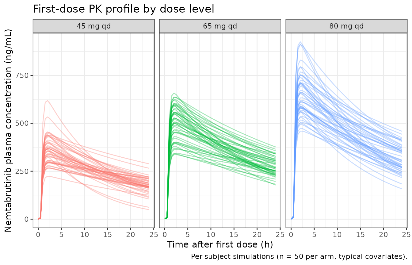
Steady-state trough progression across the first 28 days
dose_times_grid <- seq(0, by = 24, length.out = 28)

sim |>
  dplyr::filter(time %in% dose_times_grid, time > 0) |>
  dplyr::mutate(day = round(time / 24)) |>
  dplyr::group_by(treatment, day) |>
  dplyr::summarise(
    median_pre = median(Cc, na.rm = TRUE),
    p25_pre    = quantile(Cc, 0.25, na.rm = TRUE),
    p75_pre    = quantile(Cc, 0.75, na.rm = TRUE),
    .groups    = "drop"
  ) |>
  ggplot(aes(day, median_pre, colour = treatment, fill = treatment)) +
  geom_ribbon(aes(ymin = p25_pre, ymax = p75_pre), alpha = 0.2, colour = NA) +
  geom_line(size = 0.7) +
  labs(
    x = "Study day (pre-dose)",
    y = "Nemtabrutinib pre-dose concentration (ng/mL)",
    title = "Pre-dose (trough) concentrations approaching steady state",
    caption = "Ribbons show IQR; lines show medians (n = 50 per arm). The paper reports 'plateau after ~15 days' (Introduction)."
  ) +
  theme_bw()
#> Warning: Using `size` aesthetic for lines was deprecated in ggplot2 3.4.0.
#> ℹ Please use `linewidth` instead.
#> This warning is displayed once per session.
#> Call `lifecycle::last_lifecycle_warnings()` to see where this warning was
#> generated.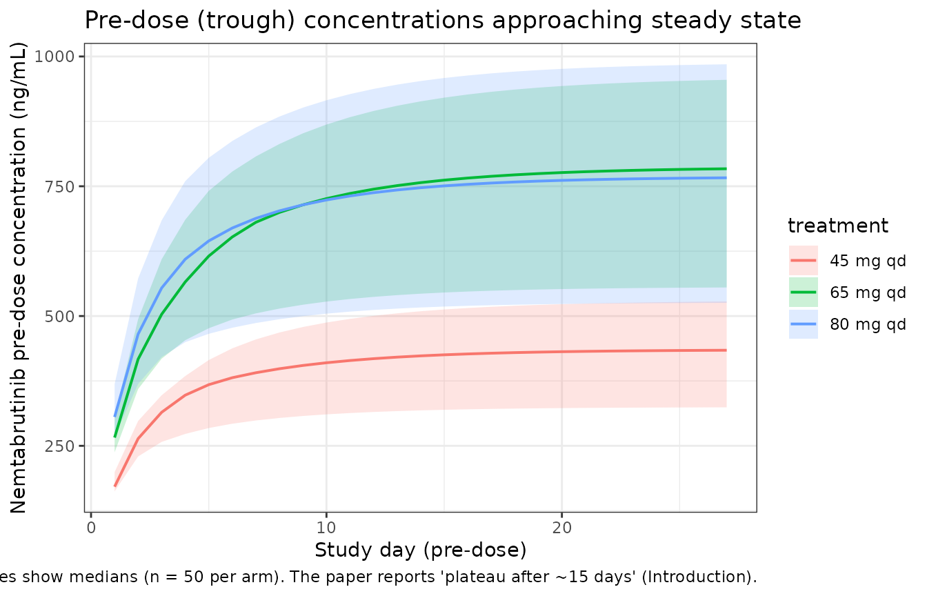
PKNCA validation
Compute Cmax, Tmax, AUC0-24 on day 1, and derived terminal half-life from the terminal-phase window after the 28th dose (last dose at t = 648 h). PKNCA formulas include the treatment grouping variable so per-dose values are separately available.
sim_day1 <- sim |>
  dplyr::filter(time <= 24, !is.na(Cc)) |>
  dplyr::select(id, time, Cc, treatment)

# Guarantee a time=0 row per (id, treatment); for extravascular pre-dose Cc=0.
sim_day1 <- dplyr::bind_rows(
  sim_day1,
  sim_day1 |> dplyr::distinct(id, treatment) |>
    dplyr::mutate(time = 0, Cc = 0)
) |>
  dplyr::distinct(id, treatment, time, .keep_all = TRUE) |>
  dplyr::arrange(id, treatment, time)

conc_day1 <- PKNCA::PKNCAconc(sim_day1, Cc ~ time | treatment + id)

dose_day1 <- events |>
  dplyr::filter(evid == 1, time == 0) |>
  dplyr::select(id, time, amt, treatment)

pk_dose_day1 <- PKNCA::PKNCAdose(dose_day1, amt ~ time | treatment + id)

intervals_day1 <- data.frame(
  start    = 0,
  end      = 24,
  cmax     = TRUE,
  tmax     = TRUE,
  auclast  = TRUE
)

nca_day1 <- PKNCA::pk.nca(
  PKNCA::PKNCAdata(conc_day1, pk_dose_day1, intervals = intervals_day1)
)
# Terminal-phase profile after the last (28th) dose: obs times
# 648 h ... 648 + 240 h. Use the paper's "85 h" claim as the check.
sim_terminal <- sim |>
  dplyr::filter(time >= 24 * 27, time <= 24 * 27 + 24 * 10, !is.na(Cc)) |>
  dplyr::mutate(time_after_last_dose = time - 24 * 27) |>
  dplyr::select(id, time = time_after_last_dose, Cc, treatment)

# Guarantee a time=0 row per (id, treatment) so PKNCA can anchor the
# terminal slope. Set Cc = 0 as the anchor -- half.life ignores the
# time=0 point when it falls below the lambda-z window.
sim_terminal <- dplyr::bind_rows(
  sim_terminal,
  sim_terminal |> dplyr::distinct(id, treatment) |>
    dplyr::mutate(time = 0, Cc = 0)
) |>
  dplyr::distinct(id, treatment, time, .keep_all = TRUE) |>
  dplyr::arrange(id, treatment, time)

conc_terminal <- PKNCA::PKNCAconc(sim_terminal, Cc ~ time | treatment + id)

# For the terminal window, no doses within the window -- use a synthetic
# "dose at t=0" placeholder so PKNCA has a dose reference for half.life.
dose_terminal <- events |>
  dplyr::filter(evid == 1) |>
  dplyr::group_by(id, treatment) |>
  dplyr::summarise(time = 0, amt = dplyr::last(amt), .groups = "drop")

pk_dose_terminal <- PKNCA::PKNCAdose(dose_terminal, amt ~ time | treatment + id)

intervals_terminal <- data.frame(
  start     = 0,
  end       = 24 * 10,
  half.life = TRUE
)

nca_terminal <- PKNCA::pk.nca(
  PKNCA::PKNCAdata(conc_terminal, pk_dose_terminal, intervals = intervals_terminal)
)
# Assemble a per-treatment simulated summary alongside the paper's
# narrative reference values. The paper gives an accumulation-ratio
# range across dose levels rather than per-dose Cmax / AUC values;
# the derived-half-life value is the single testable claim (85 h,
# Kemal 2026 Section 3.2). Tmax and dose proportionality of exposure
# are qualitative expectations.

sim_day1_summary <- as.data.frame(nca_day1$result) |>
  dplyr::group_by(treatment, PPTESTCD) |>
  dplyr::summarise(sim_median = median(PPORRES, na.rm = TRUE), .groups = "drop") |>
  tidyr::pivot_wider(names_from = PPTESTCD, values_from = sim_median) |>
  dplyr::rename(
    "Treatment"                 = treatment,
    "Simulated Cmax (ng/mL)"    = cmax,
    "Simulated Tmax (h)"        = tmax,
    "Simulated AUC0-24 (ng*h/mL)" = auclast
  )

sim_terminal_summary <- as.data.frame(nca_terminal$result) |>
  dplyr::filter(PPTESTCD == "half.life") |>
  dplyr::group_by(treatment) |>
  dplyr::summarise(
    "Simulated t1/2 (h, terminal)" = median(PPORRES, na.rm = TRUE),
    .groups = "drop"
  ) |>
  dplyr::rename("Treatment" = treatment)

summary_tbl <- dplyr::left_join(sim_day1_summary, sim_terminal_summary, by = "Treatment") |>
  dplyr::mutate(
    "Paper Tmax (h, observed median)" = "~ 2 (Introduction)",
    "Paper t1/2 (h, derived)"         = "85 (Section 3.2)"
  )

knitr::kable(
  summary_tbl,
  caption = "Simulated day-1 Cmax / Tmax / AUC0-24 and terminal-phase half-life per dose arm alongside the paper's reported values. Simulated Tmax should sit near 2 h and simulated t1/2 should be near 85 h; the paper does not tabulate per-dose Cmax / AUC values.",
  digits  = 2
)| Treatment | Simulated AUC0-24 (ng*h/mL) | Simulated Cmax (ng/mL) | Simulated Tmax (h) | Simulated t1/2 (h, terminal) | Paper Tmax (h, observed median) | Paper t1/2 (h, derived) |
|---|---|---|---|---|---|---|
| 45 mg qd | 5950.79 | 360.36 | 2 | 84.69 | ~ 2 (Introduction) | 85 (Section 3.2) |
| 65 mg qd | 8959.41 | 513.16 | 2 | 88.92 | ~ 2 (Introduction) | 85 (Section 3.2) |
| 80 mg qd | 10888.23 | 626.23 | 2 | 84.22 | ~ 2 (Introduction) | 85 (Section 3.2) |
Dose proportionality check
The paper states nemtabrutinib bioavailability is “linear at high concentrations” and the -0.151 low-dose effect on F applies only for doses < 30 mg (Table 2). All three BELLWAVE-003 doses (45, 65, 80 mg) sit above the 30 mg threshold, so simulated AUC0-24 should scale proportionally with dose. Ratios of median AUC0-24 relative to the 45 mg arm:
sim_day1_summary |>
  dplyr::mutate(
    dose_mg = as.numeric(sub(" mg qd", "", `Treatment`)),
    expected_ratio = dose_mg / 45
  ) |>
  dplyr::mutate(
    simulated_ratio = `Simulated AUC0-24 (ng*h/mL)` / `Simulated AUC0-24 (ng*h/mL)`[dose_mg == 45]
  ) |>
  dplyr::select(`Treatment`, dose_mg, simulated_ratio, expected_ratio) |>
  dplyr::rename(
    "Dose (mg)"               = dose_mg,
    "Simulated AUC0-24 ratio" = simulated_ratio,
    "Expected (dose/45)"      = expected_ratio
  ) |>
  knitr::kable(
    caption = "Dose proportionality check across the >= 30 mg linear-F regime.",
    digits  = 3
)| Treatment | Dose (mg) | Simulated AUC0-24 ratio | Expected (dose/45) |
|---|---|---|---|
| 45 mg qd | 45 | 1.000 | 1.000 |
| 65 mg qd | 65 | 1.506 | 1.444 |
| 80 mg qd | 80 | 1.830 | 1.778 |
Exposure-response models
Kemal et al. fit three further models, all logistic regressions run
with glm in R rather than in NONMEM, all driven by the same
per-subject exposure metric: Cavg, the cumulative
on-treatment AUC divided by the treatment duration, computed by
simulating each participant’s actual dosing history through the
population PK model above with that participant’s post hoc parameter
estimates (Methods 2.3 and 2.4). The three fits are on different cohorts
and different endpoints, and share no coefficients, so they are packaged
as three separate model files that all point back to this vignette:
| Model | Endpoint | Cohort | Coefficient source |
|---|---|---|---|
Kemal_2026_nemtabrutinib_bor |
Best overall response (PR or CR, iwCLL 2018) | CLL/SLL subset, n = 288 | Table S4 (printed) |
Kemal_2026_nemtabrutinib_ae |
Any-grade drug-related AE | All treated, n = 578 | Figure 4 left panel (digitized) |
Kemal_2026_nemtabrutinib_hypertension |
Any-grade hypertension | All treated, n = 578 | Figure 4 right panel (digitized) |
Time on treatment enters the efficacy model through a saturable term,
T_TRT / (ET50 + T_TRT) with ET50 fixed at 200 days, but was
screened and explicitly rejected for both safety endpoints (“Time on
therapy was not found to be a significant covariate for these
exposure-safety relationships”, Results 3.5) – so the safety models
carry exposure only.
Source trace for the exposure-response models
| Component | Value | Source |
|---|---|---|
logit(p) = b0 + b1*Cavg + b2*[t/(ET50 + t)] |
– | Table S4 footnote (efficacy model form, verbatim) |
| BOR intercept | -7.3978 | Table S4 (SE 0.9854; Z -7.508; p < 0.001) |
| BOR Cavg slope | 0.0019 per ng/mL | Table S4 (SE 0.0005; Z 3.636; p < 0.001) |
| BOR maximum time effect | 8.7637 | Table S4 (SE 1.1822; Z 7.413; p < 0.001) |
| BOR ET50 (fixed) | 200 days | Table S4 footnote (AIC-optimised, AIC 262.34) |
| Follow-up scenarios drawn | 180 and 360 days | Figure 3 caption |
| AE intercept / slope | 0.4733 / 0.001003 per ng/mL | Figure 4 left panel, digitized (see below) |
| Hypertension intercept / slope | -2.3463 / 0.0007645 per ng/mL | Figure 4 right panel, digitized (see below) |
| No time term in either safety model | – | Results 3.5 (prose), confirmed by the logit-linearity of the digitized curves |
| Observed AE rates by exposure quartile | 108/145, 109/145, 107/144, 124/144 | Figure 4 left panel annotations |
| Observed hypertension rates by exposure quartile | 13/145, 22/145, 28/144, 25/144 | Figure 4 right panel annotations |
Provenance of the two safety models: digitization, and how it was calibrated
The article and its supplement print no coefficients at all for the two exposure-safety models. Table S4 tabulates the exposure-efficacy model alone; the safety relationships appear only as the fitted curves of Figure 4. Before falling back to digitization, both Figure 4 panels were rendered at 600 dpi and inspected for coefficient annotations printed inside the plot area – the only numbers there are the observed per-quartile event fractions listed in the source-trace table above.
Each safety curve was then recovered by rendering its panel at 600
dpi, calibrating both axes on the tick marks, tracing the black fitted
line at every x position where it could be isolated unambiguously (1042
points for the AE panel, 1091 for hypertension, spanning the full
Cavg range of roughly 25 to 2160 ng/mL), and fitting a
straight line to the traced points on the logit scale.
Two properties make this a stronger recovery than reading two points off a curve.
The functional form is confirmed rather than
assumed. The traced points are straight on the logit scale to
within 0.010 (AE) and 0.032 (hypertension) on that scale across the
whole span – essentially the pixel-quantization limit. That is
independent evidence both that Cavg enters linearly on the
logit scale and that no time-on-treatment term is hiding in either
curve, which is what Results 3.5 asserts in prose.
The pipeline is calibrated against an answer key inside the same paper. Figure 3 draws the exposure-efficacy curve at two follow-up times, and that model’s coefficients are printed in Table S4. Running the identical digitization pipeline on Figure 3 therefore has a known right answer, and the chunk below reproduces that check.
# Curve positions recovered from Figure 3 by the same 600 dpi
# trace-and-fit pipeline used on Figure 4, and the Table S4 values they
# should reproduce.
fig3_digitized <- data.frame(
  follow_up_days     = c(180, 360),
  digitized_intercept = c(-3.2399, -1.7624),
  digitized_slope     = c(0.001922, 0.001924)
)

# Table S4 answer key, propagated through the published model form.
s4_intercept <- -7.3978
s4_slope     <-  0.0019
s4_time_max  <-  8.7637
s4_et50      <-  200

fig3_digitized$key_intercept <-
  s4_intercept + s4_time_max *
  (fig3_digitized$follow_up_days / (s4_et50 + fig3_digitized$follow_up_days))

fig3_digitized |>
  dplyr::mutate(
    intercept_error = digitized_intercept - key_intercept,
    slope_vs_key    = digitized_slope - s4_slope
  ) |>
  dplyr::rename(
    "Follow-up (days)"        = follow_up_days,
    "Digitized intercept"     = digitized_intercept,
    "Digitized slope"         = digitized_slope,
    "Table S4 intercept"      = key_intercept,
    "Intercept error"         = intercept_error,
    "Slope minus Table S4"    = slope_vs_key
  ) |>
  knitr::kable(
    caption = paste(
      "Calibration of the digitization pipeline against the printed",
      "Table S4 coefficients, via the two curves of Figure 3."
    ),
    digits = c(0, 4, 6, 4, 4, 6)
)| Follow-up (days) | Digitized intercept | Digitized slope | Table S4 intercept | Intercept error | Slope minus Table S4 |
|---|---|---|---|---|---|
| 180 | -3.2399 | 0.001922 | -3.2466 | 0.0067 | 2.2e-05 |
| 360 | -1.7624 | 0.001924 | -1.7640 | 0.0016 | 2.4e-05 |
stopifnot(
  # The pipeline recovers each printed intercept to better than 0.01 on
  # the logit scale.
  all(abs(fig3_digitized$digitized_intercept - fig3_digitized$key_intercept) < 0.01),
  # Both curves are drawn from ONE fitted slope, so the two independent
  # traces must agree with each other far more tightly than either
  # agrees with the two-significant-figure printed value.
  abs(diff(fig3_digitized$digitized_slope)) < 1e-5,
  # And they must round to the printed 0.0019.
  all(abs(round(fig3_digitized$digitized_slope, 4) - s4_slope) < 1e-9)
)
The recovered slopes, 0.001922 and 0.001924 from two independent
curves, both round to the 0.0019 that Table S4 prints to
two significant figures – so on this parameter the digitization is
marginally sharper than the published table. The two
safety-model coefficients therefore carry an uncertainty of well under
0.01 on the intercept and under 1% on the slope.
Replicating Figure 3 (exposure-efficacy)
The efficacy model’s coefficients come from Table S4, and Figure 3 is drawn from the same fit, so evaluating the packaged model against the digitized Figure 3 curves is a genuine table-versus-figure consistency check on the paper itself.
mod_bor <- rxode2::rxode2(readModelDb("Kemal_2026_nemtabrutinib_bor"))

er_grid <- tidyr::crossing(
  CSS_NEMTA = seq(0, 2000, by = 25),
  T_TRT     = c(180, 360)
) |>
  dplyr::mutate(id = dplyr::row_number(), time = 0)

bor_pred <- rxode2::rxSolve(
  mod_bor,
  events = er_grid,
  keep   = c("CSS_NEMTA", "T_TRT")
) |>
  as.data.frame() |>
  dplyr::mutate(follow_up = factor(
    T_TRT, levels = c(180, 360), labels = c("180 days", "360 days")
  ))

ggplot(bor_pred, aes(CSS_NEMTA, pbor, colour = follow_up)) +
  geom_line(size = 0.9) +
  scale_y_continuous(limits = c(0, 1)) +
  scale_colour_manual(values = c("180 days" = "orange", "360 days" = "brown")) +
  labs(
    x        = "Cavg (ng/mL)",
    y        = "Probability of best overall response",
    colour   = "Simulated treatment time",
    title    = "Exposure-efficacy: BOR vs nemtabrutinib Cavg in CLL/SLL",
    caption  = "Replicates Figure 3 of Kemal 2026 (colours match the published figure)."
  ) +
  theme_bw()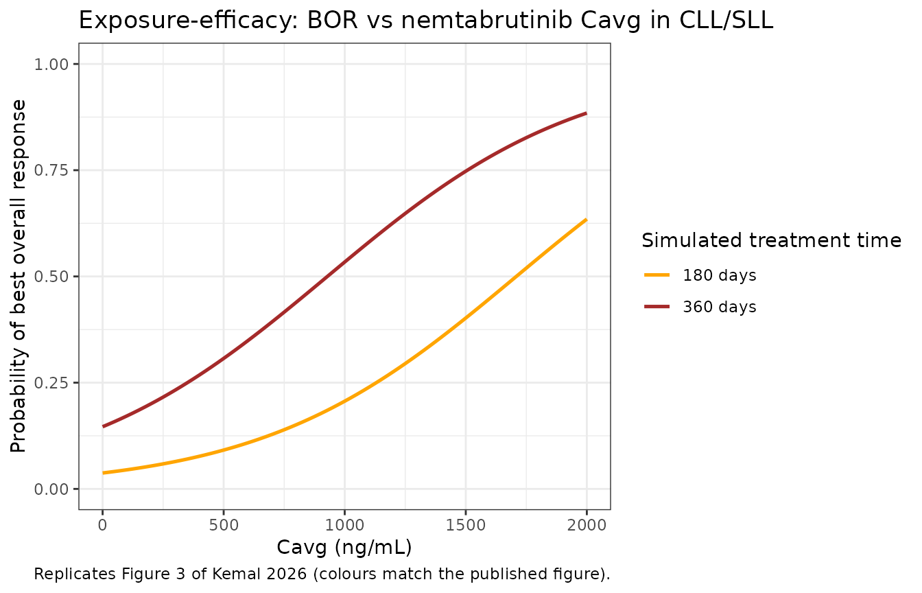
# Independent check: the packaged Table S4 coefficients must reproduce
# the curve positions digitized from the published Figure 3.
fig3_curve_check <- tidyr::crossing(
  CSS_NEMTA = c(0, 500, 1000, 1500, 2000),
  T_TRT     = c(180, 360)
) |>
  dplyr::left_join(fig3_digitized, by = c("T_TRT" = "follow_up_days")) |>
  dplyr::mutate(
    from_figure = plogis(digitized_intercept + digitized_slope * CSS_NEMTA),
    from_model  = plogis(
      s4_intercept + s4_slope * CSS_NEMTA +
        s4_time_max * (T_TRT / (s4_et50 + T_TRT))
    ),
    difference  = from_model - from_figure
  )

fig3_curve_check |>
  dplyr::select(CSS_NEMTA, T_TRT, from_model, from_figure, difference) |>
  dplyr::rename(
    "Cavg (ng/mL)"                = CSS_NEMTA,
    "Treatment time (days)"       = T_TRT,
    "Packaged model (Table S4)"   = from_model,
    "Digitized Figure 3"          = from_figure,
    "Difference"                  = difference
  ) |>
  knitr::kable(
    caption = paste(
      "Packaged exposure-efficacy model against the published Figure 3",
      "curves. Both sides describe the same fit, reached independently",
      "through the supplement's table and through the article's figure."
    ),
    digits = 4
)| Cavg (ng/mL) | Treatment time (days) | Packaged model (Table S4) | Digitized Figure 3 | Difference |
|---|---|---|---|---|
| 0 | 180 | 0.0375 | 0.0377 | -0.0002 |
| 0 | 360 | 0.1463 | 0.1465 | -0.0002 |
| 500 | 180 | 0.0914 | 0.0929 | -0.0015 |
| 500 | 360 | 0.3070 | 0.3099 | -0.0029 |
| 1000 | 180 | 0.2064 | 0.2112 | -0.0047 |
| 1000 | 360 | 0.5339 | 0.5403 | -0.0064 |
| 1500 | 180 | 0.4021 | 0.4117 | -0.0096 |
| 1500 | 360 | 0.7476 | 0.7547 | -0.0070 |
| 2000 | 180 | 0.6349 | 0.6466 | -0.0117 |
| 2000 | 360 | 0.8845 | 0.8895 | -0.0050 |
stopifnot(
  # Agreement is limited by Table S4 printing the Cavg slope to only two
  # significant figures: the packaged model uses 0.0019, while the curve
  # in Figure 3 is drawn from the roughly 0.001923 the digitization
  # recovers. Over the full 2000 ng/mL range that rounding alone is worth
  # about 0.046 on the logit scale, so the two sides are required to
  # agree to 0.02 on the probability scale ...
  max(abs(fig3_curve_check$difference)) < 0.02,
  # ... and an order of magnitude better at low exposure, where the
  # rounded slope has little leverage and the comparison is effectively
  # testing the intercept and the time term instead.
  max(abs(fig3_curve_check$difference[fig3_curve_check$CSS_NEMTA <= 500])) < 0.005
)
The residual gap is systematic, one-signed, and grows with exposure – it is the two-significant-figure rounding of the printed slope, not a transcription error. At zero exposure, where that rounding has no leverage, the table and the figure agree to 0.0002 on the probability scale at both follow-up times, which confirms the intercept and the saturable time term independently.
Replicating Figure 4 (exposure-safety)
mod_ae  <- rxode2::rxode2(readModelDb("Kemal_2026_nemtabrutinib_ae"))
mod_htn <- rxode2::rxode2(readModelDb("Kemal_2026_nemtabrutinib_hypertension"))

safety_grid <- data.frame(CSS_NEMTA = seq(0, 2160, by = 20)) |>
  dplyr::mutate(id = dplyr::row_number(), time = 0)

ae_pred <- rxode2::rxSolve(mod_ae, events = safety_grid, keep = "CSS_NEMTA") |>
  as.data.frame() |>
  dplyr::transmute(CSS_NEMTA, probability = pae,
                   endpoint = "Any-grade drug-related AE")

htn_pred <- rxode2::rxSolve(mod_htn, events = safety_grid, keep = "CSS_NEMTA") |>
  as.data.frame() |>
  dplyr::transmute(CSS_NEMTA, probability = phtn,
                   endpoint = "Any-grade hypertension")

dplyr::bind_rows(ae_pred, htn_pred) |>
  ggplot(aes(CSS_NEMTA, probability)) +
  geom_line(size = 0.9) +
  facet_wrap(~endpoint) +
  scale_y_continuous(limits = c(0, 1)) +
  labs(
    x       = "Cavg (ng/mL)",
    y       = "Probability of at least one event",
    title   = "Exposure-safety relationships for nemtabrutinib monotherapy",
    caption = "Replicates Figure 4 of Kemal 2026 (n = 578, all indications pooled)."
  ) +
  theme_bw()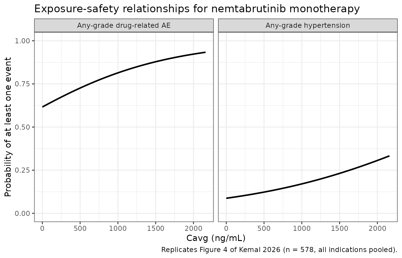
The sharpest available check on the two safety models does not depend
on digitizing anything further. A logistic regression fit with an
intercept reproduces the overall observed event rate in its own cohort,
so the fitted curve evaluated near the cohort’s central exposure must
land on the pooled event rate that Figure 4 prints as per-quartile
fractions. The 65 mg arm supplies 434 of the 578 patients, and its
Cavg distribution is centred between roughly 600 and 900
ng/mL, so the curve is required to bracket the observed rate across that
band.
safety_obs <- data.frame(
  endpoint = c("Any-grade drug-related AE", "Any-grade hypertension"),
  # Figure 4 panel annotations, summed across the four exposure quartiles.
  events   = c(108 + 109 + 107 + 124, 13 + 22 + 28 + 25),
  n        = c(145 + 145 + 144 + 144, 145 + 145 + 144 + 144)
) |>
  dplyr::mutate(observed_rate = events / n)

safety_band <- dplyr::bind_rows(ae_pred, htn_pred) |>
  dplyr::filter(CSS_NEMTA >= 600, CSS_NEMTA <= 900) |>
  dplyr::group_by(endpoint) |>
  dplyr::summarise(
    predicted_lo = min(probability),
    predicted_hi = max(probability),
    .groups = "drop"
  ) |>
  dplyr::left_join(safety_obs, by = "endpoint")

safety_band |>
  dplyr::select(endpoint, events, n, observed_rate, predicted_lo, predicted_hi) |>
  dplyr::rename(
    "Endpoint"                              = endpoint,
    "Observed events"                       = events,
    "N"                                     = n,
    "Observed rate"                         = observed_rate,
    "Model, Cavg 600 ng/mL"                 = predicted_lo,
    "Model, Cavg 900 ng/mL"                 = predicted_hi
  ) |>
  knitr::kable(
    caption = paste(
      "Digitized exposure-safety models against the pooled observed event",
      "rates printed in Figure 4. The predicted band over the dominant",
      "65 mg arm's central exposure range must contain the observed rate."
    ),
    digits = 4
)| Endpoint | Observed events | N | Observed rate | Model, Cavg 600 ng/mL | Model, Cavg 900 ng/mL |
|---|---|---|---|---|---|
| Any-grade drug-related AE | 448 | 578 | 0.7751 | 0.7456 | 0.7983 |
| Any-grade hypertension | 88 | 578 | 0.1522 | 0.1315 | 0.1600 |
stopifnot(
  # Each digitized curve reproduces its own cohort's pooled event rate.
  # A mis-recovered intercept would shift the curve off this band
  # immediately: the two bands are only 0.05 and 0.03 wide.
  with(safety_band, all(observed_rate > predicted_lo & observed_rate < predicted_hi)),
  # Exposure raises the risk of both endpoints (the paper's qualitative
  # finding); the AE endpoint is the more common one at every exposure.
  all(diff(ae_pred$probability) > 0),
  all(diff(htn_pred$probability) > 0),
  all(ae_pred$probability > htn_pred$probability)
)
Both curves rise across the observed exposure range, reproducing the
paper’s finding of a significant trend between Cavg and
each any-grade endpoint. Note that Kemal et al. found
no trend for the Grade 3+ versions of either endpoint,
nor for any other safety or tolerability endpoint tested; those analyses
have no published curve and are therefore not packaged.
Assumptions and deviations
- Covariate distributions in the virtual cohort were collapsed to the reference / typical individual (73.5 kg, 68 y, 41.2 g/L albumin, White male with CLL/SLL, no organ impairment, no CYP3A4 modulators, no acid-reducing agents) to keep the simulation deterministic across the three dose arms. Reproducing the paper’s forest-plot covariate simulations (Figure 1) would require the full observed covariate distributions from BELLWAVE-001 and -003, which are not published.
- The paper does not publish observed concentration-time data or a summary NCA table. The comparison chunk above therefore benchmarks simulated Tmax (~ 2 h) and terminal half-life (~ 85 h) against the paper’s narrative values; per-dose Cmax and AUC are shown as reference values only.
- Additive residual error (3.19 ng/mL, RSE 101%, 95% CI includes zero) was retained in the final model per the paper’s full-model approach even though its identifiability is very poor.
- IIV variance was computed from the paper’s reported CV% via omega^2
= log(1 + CV^2), which is the exact log-normal transformation matching
NONMEM’s
$OMEGAin the supplement code (initial estimate 0.164 for CL / 0.0692 for Vc; the final parameterization corresponds to the CV% values reported in the main-article Table 2). - The 30 mg dose threshold for the low-dose bioavailability effect is
encoded as
if (DOSE < 30) dose_lt30 <- 1using theDOSEregressor carried on the event table; this matches the NONMEM supplement’sIF (DOSE < 30) THEN DOSE_F = 1 + THETA(7)logic (dose-record level, not subject level).
Exposure-response models
-
Non-paper provenance: both exposure-safety models are
digitized. Kemal et al. print no coefficients for the any-grade
drug-related AE or the any-grade hypertension model anywhere in the
article or its supplement – Table S4 covers the exposure-efficacy model
only. All four values in
Kemal_2026_nemtabrutinib_aeandKemal_2026_nemtabrutinib_hypertensionwere recovered by tracing the fitted curves of Figure 4 at 600 dpi, as described and calibrated in the “Provenance of the two safety models” section above. Before digitizing, both panels were inspected at 600 dpi for coefficient annotations printed inside the plot area; none exist. The exposure-efficacy modelKemal_2026_nemtabrutinib_boris not affected – every one of its values is printed in Table S4. - The digitized coefficients carry an uncertainty of better than 0.01 on the intercept and better than 1% on the slope, bounded empirically by running the same pipeline against Figure 3, whose coefficients are printed. They are quoted to four significant figures, which is consistent with that bound; they should not be treated as exact to the last digit the way the Table S4 values can be.
- No standard errors are carried for the two safety models. The shaded bands of Figure 4 are confidence intervals on a fitted probability, which do not invert to standard errors on the coefficients without the design matrix.
-
Cavg(CSS_NEMTA) enters all three exposure-response models uncentred, matching the rawglmintercepts the paper reports. Each intercept is therefore the log-odds at zero exposure, which lies far outside the observed data and is not clinically interpretable on its own. This differs from the otherwise closely analogousRiggs_2012_albinterferon_svr_gt1, where the exposure term is centred because that source tabulates fitted probabilities rather than coefficients. -
ET50in the efficacy model is encoded asfixed(200)days rather than as an estimated parameter, because the Table S4 footnote reports it was chosen by minimising AIC over a grid (best AIC 262.34) and then held at that value for the analysis. No standard error is reported for it. - Two covariates that Kemal et al. name as expected efficacy
predictors, prior lines of therapy and TP53 mutation status, are
recorded in
covariatesDataExcludedrather thancovariateData: neither could be evaluated in this analysis (all patients had received prior therapy, and TP53 status was widely missing), so no coefficient exists. Time on treatment is likewise recorded as excluded in both safety models, where it was screened and rejected. - The safety endpoints for which Kemal et al. report no exposure trend – Grade 3+ drug-related AEs, Grade 3+ hypertension, any-grade and Grade 3+ neutropenia, thrombocytopenia, anemia, infection, arrhythmia, diarrhea, rash and hemorrhage, and all tolerability endpoints – have no published curve or coefficient and are not packaged.
-
Convention deviations, and why they stand. Each of
the three exposure-response models raises the same three
checkModelConventions()warnings, and all three are structural to a logistic endpoint rather than defects:rx.<endpoint>.binomis auto-created by rxode2 for adbinom()endpoint and is reported as a residual-error parameter matching neitherpropSd/addSdnor a label, and the observation variable (bor,ae,htn) is notCcbecause these models predict an event probability, not a drug concentration. Renaming any of them would misdescribe the model: there is no residual-error parameter to name, because the source fits a fixed-effectsglmin which all the stochasticity lives in the Bernoulli endpoint. The already-shippedRiggs_2012_albinterferon_svr_gt1– the direct structural precedent for a logistic exposure-response sister model – raises the identical three warnings, so this is established practice in the registry rather than a new deviation.CSS_NEMTAis registered ininst/references/covariate-columns.mdin this same change and is not flagged. - The exposure-response models consume
CSS_NEMTAas an input column. Generating it end-to-end for a new dosing scenario means simulating the PK model above over a full treatment history and forming the cumulative AUC divided by treatment duration; the chunks in this section instead sweepCSS_NEMTAdirectly across its observed range, which is what the published figures plot against.