Oseltamivir exposure-response for influenza efficacy (Rayner 2013)

Models and source

Rayner 2013 reports three independently-fitted final exposure-response models, one per efficacy endpoint, so the paper contributes three model files that share this one vignette.

mods <- c(
  symptomscore     = "Rayner_2013_oseltamivir_symptomscore",
  symptomalleviation = "Rayner_2013_oseltamivir_symptomalleviation",
  shedding         = "Rayner_2013_oseltamivir_shedding"
)
ui <- lapply(mods, function(n) rxode2::rxode(readModelDb(n)))

tibble::tibble(
  Endpoint = c(
    "Composite symptom score AUC (continuous)",
    "Time to alleviation of composite symptom score (time-to-event)",
    "Time to cessation of viral shedding (time-to-event)"
  ),
  Model = unname(mods),
  Method = c(
    "Linear regression",
    "Cox proportional hazards",
    "Cox proportional hazards"
  ),
  Subjects = vapply(ui, function(u) u$population$n_subjects, integer(1))
) |>
  knitr::kable(caption = "The three final multivariable models of Rayner 2013 Table 6.")

The three final multivariable models of Rayner 2013 Table 6.

Endpoint	Model	Method	Subjects
Composite symptom score AUC (continuous)	Rayner_2013_oseltamivir_symptomscore	Linear regression	112
Time to alleviation of composite symptom score (time-to-event)	Rayner_2013_oseltamivir_symptomalleviation	Cox proportional hazards	64
Time to cessation of viral shedding (time-to-event)	Rayner_2013_oseltamivir_shedding	Cox proportional hazards	92

• Citation: Rayner CR, Bulik CC, Kamal MA, Reynolds DK, Toovey S, Hammel JP, Smith PF, Bhavnani SM, Van Wart SA, Ambrose PG, Forrest A. Pharmacokinetic-pharmacodynamic determinants of oseltamivir efficacy using data from phase 2 inoculation studies. Antimicrob Agents Chemother. 2013;57(8):3478-3487. doi:10.1128/AAC.02440-12. Parameter estimates are from Table 6 (final multivariable model); the reference-cohort level is from Table 4 and the univariable cross-check estimates are from Table 3. The upstream population PK model that generates the OC AUC0-24 covariate is Kamal MA et al. Antimicrob Agents Chemother. 2013;57(8):3470-3477, doi:10.1128/AAC.02438-12; see modellib(‘Kamal_2013_oseltamivir’).
• Article: https://doi.org/10.1128/AAC.02440-12
• Companion population PK paper (source of the exposure covariate): https://doi.org/10.1128/AAC.02438-12, packaged as modellib("Kamal_2013_oseltamivir")

The full descriptions are in the model metadata:

for (n in names(mods)) {
  cat("\n**", mods[[n]], "**\n\n", ui[[n]]$description, "\n", sep = "")
}

Rayner_2013_oseltamivir_symptomscore

Exposure-response linear-regression model for the area under the composite influenza symptom score curve (AUCSC) over 9 days in healthy adults experimentally inoculated with influenza A/Texas/36/91 (H1N1) or B/Yamagata/16/88 and treated with oral oseltamivir or placebo (Rayner 2013, pooled phase 2 inoculation studies PV15616 and NP15717). The exposure driver is the steady-state (day-5) AUC from 0 to 24 h of the active metabolite oseltamivir carboxylate (OC), taken as a per-subject input covariate from post hoc estimates of the companion population PK model (Kamal 2013; available as modellib(‘Kamal_2013_oseltamivir’)). OC AUC0-24 enters as a 3-group categorical variable with cutoffs 1,495 and 14,497 ng*h/mL, which the authors determined by minimising the likelihood- ratio P value; the neuraminidase-inhibition IC50 of the infecting strain (0.18 vs 16.76 nM, a surrogate for study and virus type) is retained as a second covariate although it is not statistically significant. The model is algebraic and deterministic (no ODE state, no drug input, no IIV, no residual error): it returns the predicted AUCSC and the predicted contrast against the lowest-exposure reference cohort. Companion time-to-event models from the same paper are modellib(‘Rayner_2013_oseltamivir_symptomalleviation’) and modellib(‘Rayner_2013_oseltamivir_shedding’).

Rayner_2013_oseltamivir_symptomalleviation

Cox proportional-hazards exposure-response model for the time to alleviation of the composite influenza symptom score in healthy adults experimentally inoculated with influenza A/Texas/36/91 (H1N1) or B/Yamagata/16/88 and treated with oral oseltamivir or placebo (Rayner 2013, pooled phase 2 inoculation studies PV15616 and NP15717). The exposure driver is the steady-state (day-5) AUC from 0 to 24 h of the active metabolite oseltamivir carboxylate (OC), taken as a per-subject input covariate from post hoc estimates of the companion population PK model (Kamal 2013; available as modellib(‘Kamal_2013_oseltamivir’)). OC AUC0-24 enters as a 3-group categorical variable with cutoffs 1,568 and 13,638 ng*h/mL; the neuraminidase-inhibition IC50 of the infecting strain (0.18 vs 16.76 nM, a surrogate for study and virus type) is retained as a second covariate although it is not statistically significant. A higher hazard means EARLIER symptom alleviation, so the hazard ratios above 1 for the middle (1.85) and high (5.34) exposure groups mean faster recovery with increasing OC exposure. Because the fit is a semiparametric Cox regression, the baseline hazard is unspecified by construction and is not reported; the model therefore returns the RELATIVE hazard hr against the lowest-exposure influenza A reference cohort, not an absolute survivor function. Multiply hr by any user-supplied baseline hazard h0(t) to obtain a subject hazard. The model is algebraic and deterministic (no ODE state, no drug input, no IIV, no residual error). Companion models from the same paper are modellib(‘Rayner_2013_oseltamivir_symptomscore’) and modellib(‘Rayner_2013_oseltamivir_shedding’).

Rayner_2013_oseltamivir_shedding

Cox proportional-hazards exposure-response model for the time to cessation of influenza virus shedding in healthy adults experimentally inoculated with influenza A/Texas/36/91 (H1N1) or B/Yamagata/16/88 and treated with oral oseltamivir or placebo (Rayner 2013, pooled phase 2 inoculation studies PV15616 and NP15717). The exposure driver is the steady-state (day-5) AUC from 0 to 24 h of the active metabolite oseltamivir carboxylate (OC), taken as a per-subject input covariate from post hoc estimates of the companion population PK model (Kamal 2013; available as modellib(‘Kamal_2013_oseltamivir’)). OC AUC0-24 enters as a 3-group categorical variable whose reference level is zero exposure (placebo) and whose upper cutoff is 14,180 ng*h/mL; the neuraminidase-inhibition IC50 of the infecting strain (0.18 vs 16.76 nM, a surrogate for study and virus type) is retained as a second covariate although it is not statistically significant. A higher hazard means EARLIER cessation of shedding, so the hazard ratios above 1 for the drug-treated (1.72) and high-exposure (2.42) groups mean faster viral clearance with increasing OC exposure. Because the fit is a semiparametric Cox regression, the baseline hazard is unspecified by construction and is not reported; the model therefore returns the RELATIVE hazard hr against the placebo reference cohort, not an absolute survivor function. Multiply hr by any user-supplied baseline hazard h0(t) to obtain a subject hazard. The model is algebraic and deterministic (no ODE state, no drug input, no IIV, no residual error). Companion models from the same paper are modellib(‘Rayner_2013_oseltamivir_symptomscore’) and modellib(‘Rayner_2013_oseltamivir_symptomalleviation’).

Population

Data came from two phase 2 experimental-inoculation studies in healthy adult volunteers. Study 1 (PV15616) inoculated 69 evaluable subjects with influenza A/Texas/36/91 (H1N1) and randomised them to placebo or oral oseltamivir 20 mg BID, 100 mg BID, 200 mg QD or 200 mg BID for 5 days, with treatment starting 28 h after inoculation. Study 2 (NP15717) inoculated 46 evaluable subjects with influenza B/Yamagata/16/88 and randomised them to placebo or oseltamivir 75 mg BID or 150 mg BID for 5 days. Pooled baseline characteristics (Rayner 2013 Table 1) were mean age 23.4 years (CV 25.4%), mean weight 70.6 kg (CV 18.0%), mean height 172 cm (CV 5.45%) and mean creatinine clearance 114 mL/min/1.73 m^2 (CV 22.2%); 51% were female and 84.4% White, 6.96% Black and 8.70% Other. Subjects had to be seronegative or nearly so at entry (antibody titre 1:8 or less in study 1, below 1:10 in study 2).

The three endpoints used different evaluable subsets, which is why the three model files carry different n_subjects (112, 64 and 92 from the Rayner 2013 Table 4 subgroup counts). The same information is available programmatically via each model’s population metadata, for example rxode2::rxode(readModelDb("Rayner_2013_oseltamivir_symptomscore"))$population.

tibble::tibble(
  Characteristic = c("Age (yr)", "Height (cm)", "Weight (kg)",
                     "Creatinine clearance (mL/min/1.73 m^2)"),
  `Study 1` = c("22.3 (CV 20.3%)", "170 (CV 5.72%)",
                "68.6 (CV 20.5%)", "108 (CV 23.8%)"),
  `Study 2` = c("25.0 (CV 29.3%)", "176 (CV 4.44%)",
                "73.7 (CV 13.4%)", "124 (CV 17.8%)"),
  `Both studies` = c("23.4 (CV 25.4%)", "172 (CV 5.45%)",
                     "70.6 (CV 18.0%)", "114 (CV 22.2%)")
) |>
  knitr::kable(caption = "Rayner 2013 Table 1, baseline demographics of the evaluable subjects.")

Rayner 2013 Table 1, baseline demographics of the evaluable subjects.

Characteristic	Study 1	Study 2	Both studies
Age (yr)	22.3 (CV 20.3%)	25.0 (CV 29.3%)	23.4 (CV 25.4%)
Height (cm)	170 (CV 5.72%)	176 (CV 4.44%)	172 (CV 5.45%)
Weight (kg)	68.6 (CV 20.5%)	73.7 (CV 13.4%)	70.6 (CV 18.0%)
Creatinine clearance (mL/min/1.73 m^2)	108 (CV 23.8%)	124 (CV 17.8%)	114 (CV 22.2%)

Model structure

All three models share the same covariate structure, which is the paper’s central design choice: the continuous exposure variable is collapsed into a 3-group categorical variable using a pair of cutoffs the authors optimised per endpoint, and the neuraminidase-inhibition IC50 of the infecting strain is carried as a two-level categorical variable.

• AUC_OSELCARB – steady-state (day-5) oseltamivir carboxylate AUC from 0 to 24 h, in ng*h/mL. Placebo subjects carry exactly 0.
• IC50_NEURAMINIDASE – 0.18 nM for influenza A/Texas (the reference stratum) or 16.76 nM for influenza B/Yamagata, in nM.

The continuous-to-categorical mapping lives in model() so the paper’s printed cutoffs stay visible in ini():

cut_tbl <- lapply(names(mods), function(n) {
  d <- ui[[n]]$iniDf
  tibble::tibble(
    Model = mods[[n]],
    `Lower cutoff (ng*h/mL)` = d$est[d$name == "auc_cut1"],
    `Upper cutoff (ng*h/mL)` = d$est[d$name == "auc_cut2"]
  )
}) |>
  dplyr::bind_rows()

knitr::kable(
  cut_tbl,
  caption = "Optimally-determined OC AUC0-24 3-group cutoffs (Rayner 2013 Table 6)."
)

Optimally-determined OC AUC0-24 3-group cutoffs (Rayner 2013 Table 6).

Model	Lower cutoff (ng*h/mL)	Upper cutoff (ng*h/mL)
Rayner_2013_oseltamivir_symptomscore	1495	14497
Rayner_2013_oseltamivir_symptomalleviation	1568	13638
Rayner_2013_oseltamivir_shedding	0	14180

# The paper's headline finding: the three upper cutoffs were optimised
# independently for three different endpoints and all landed near
# 14,000 ng*h/mL. This is arithmetic on printed values, so it is exact.
upper <- cut_tbl[["Upper cutoff (ng*h/mL)"]]
stopifnot(
  length(upper) == 3L,
  all(abs(upper / 14000 - 1) < 0.05)
)

Source trace

Every ini() entry carries an in-file comment naming its source location. The table below collects them.

Model	Parameter	Value	Source location
symptomscore	aucsc_int	14.6 score*day	Table 4, composite symptom score AUC, subgroup at or below 1,495 ng*h/mL (see Assumptions)
symptomscore	auc_cut1	1495 ng*h/mL	Table 6, composite symptom score AUC reference group
symptomscore	auc_cut2	14497 ng*h/mL	Table 6, composite symptom score AUC comparison group
symptomscore	e_auc_oselcarb_mid_aucsc	-5.36 score*day	Table 6 (95% CI -8.73, -1.99; P = 0.0021)
symptomscore	e_auc_oselcarb_high_aucsc	-7.03 score*day	Table 6 (95% CI -11.8, -2.27; P = 0.0042)
symptomscore	e_ic50_neuraminidase_aucsc	1.77 score*day	Table 6 (95% CI -1.31, 4.85; P = 0.257)
symptomalleviation	auc_cut1	1568 ng*h/mL	Table 6, time-to-alleviation reference group
symptomalleviation	auc_cut2	13638 ng*h/mL	Table 6, time-to-alleviation comparison group
symptomalleviation	e_auc_oselcarb_mid_haz	log(1.85)	Table 6, HR 1.85 (95% CI 1.01, 3.39; P = 0.045)
symptomalleviation	e_auc_oselcarb_high_haz	log(5.34)	Table 6, HR 5.34 (95% CI 2.37, 12.07; P < 0.001)
symptomalleviation	e_ic50_neuraminidase_haz	log(0.82)	Table 6, HR 0.82 (95% CI 0.46, 1.45; P = 0.494)
shedding	auc_cut1	0 ng*h/mL	Table 6, viral-shedding reference group
shedding	auc_cut2	14180 ng*h/mL	Table 6, viral-shedding comparison group
shedding	e_auc_oselcarb_mid_haz	log(1.72)	Table 6, HR 1.72 (95% CI 0.98, 3.03; P = 0.059)
shedding	e_auc_oselcarb_high_haz	log(2.42)	Table 6, HR 2.42 (95% CI 1.20, 4.84; P = 0.013)
shedding	e_ic50_neuraminidase_haz	log(0.66)	Table 6, HR 0.66 (95% CI 0.38, 1.14; P = 0.136)
all three	ic50_ref	0.18 nM	Table 6 IC50 reference group; assay value 0.18 +/- 0.11 nM in Methods, “NA inhibition assay”
all three	3-group indicator equations	n/a	Methods, “Univariable analyses” (cutoff optimisation) and Table 6 group boundaries
all three	AUC_OSELCARB derivation	n/a	Methods, “Determination of plasma drug exposures”

None of the parameter values are figure-derived or supplied by correspondence: all sixteen come from Tables 4 and 6 of the main paper.

Validation

The three models are algebraic and deterministic – no ODE state, no drug input, no between-subject variability and no residual error – so PKNCA is not the right validation instrument for them (following references/endogenous-validation.md, which replaces the NCA section for model classes where there is no concentration-time profile to integrate). Instead this vignette runs four checks:

A. the models reproduce Rayner 2013 Table 6 exactly; B. the group-boundary convention matches the table’s <= / > notation; C. the paper’s own tables are internally consistent, which is what identifies the otherwise-unreported reference level; and D. an end-to-end dose to exposure to response chain through the upstream Kamal 2013 population PK model, where PKNCA does apply, because the exposure covariate the three models consume is itself an NCA quantity.

A. Table 6 is reproduced exactly

Each model is evaluated on the six covariate cohorts defined by three exposure groups crossed with two infecting strains. Because the models are deterministic, these are exact-arithmetic checks.

# One representative exposure per group per model: the group midpoint is not
# needed, only a value that lands inside the group, so the reference value is
# 0 (placebo) and the other two are offsets from the printed cutoffs.
six_cohorts <- function(u) {
  d <- u$iniDf
  c1 <- d$est[d$name == "auc_cut1"]
  c2 <- d$est[d$name == "auc_cut2"]
  tidyr::expand_grid(
    exposure = c("low", "middle", "high"),
    strain = c("A/Texas", "B/Yamagata")
  ) |>
    dplyr::mutate(
      AUC_OSELCARB = dplyr::case_when(
        exposure == "low" ~ 0,
        exposure == "middle" ~ (c1 + c2) / 2,
        exposure == "high" ~ c2 * 1.5
      ),
      IC50_NEURAMINIDASE = ifelse(strain == "A/Texas", 0.18, 16.76),
      id = dplyr::row_number(),
      time = 0,
      evid = 0L,
      amt = NA_real_
    )
}

solve_static <- function(u) {
  ev <- six_cohorts(u)
  rxode2::rxSolve(
    u, ev,
    keep = c("exposure", "strain"),
    returnType = "data.frame"
  )
}

sim_six <- lapply(ui, solve_static)

s <- sim_six$symptomscore

# The exposure contrast d_aucsc is the paper's estimate and must be free of
# the strain effect, so it must be identical in both strata.
# mean(), never unique(): these are floating-point values that agree to
# machine precision but not necessarily bit-for-bit, and unique() on a float
# silently returns more than one row (failure pattern 3).
contrast <- s |>
  dplyr::group_by(exposure) |>
  dplyr::summarise(
    d_aucsc = mean(d_aucsc),
    spread = diff(range(d_aucsc)),
    .groups = "drop"
  )

stopifnot(
  nrow(contrast) == 3L,
  # The contrast must not depend on the stratum at all.
  all(contrast$spread < 1e-12),
  isTRUE(all.equal(contrast$d_aucsc[contrast$exposure == "low"], 0)),
  isTRUE(all.equal(contrast$d_aucsc[contrast$exposure == "middle"], -5.36)),
  isTRUE(all.equal(contrast$d_aucsc[contrast$exposure == "high"], -7.03))
)

# Strain effect: the B/Yamagata minus A/Texas difference must be the printed
# 1.77 score*day at every exposure level.
strain_eff <- s |>
  dplyr::select(exposure, strain, aucsc) |>
  tidyr::pivot_wider(names_from = strain, values_from = aucsc) |>
  dplyr::mutate(diff = `B/Yamagata` - `A/Texas`)
stopifnot(
  nrow(strain_eff) == 3L,
  isTRUE(all.equal(strain_eff$diff, rep(1.77, 3)))
)

# Over-determining check: Table 6 ALSO prints the high-vs-middle contrast as
# -1.68. The two coefficients above imply -7.03 - (-5.36) = -1.67. This is an
# independent transcription check on both coefficients at once, so the
# tolerance is derived from Table 6's printed precision rather than picked:
# each of -5.36, -7.03 and -1.68 is printed to two decimals, hence carries a
# half-unit rounding uncertainty of 0.005, and a difference of two such values
# compared against a third accumulates all three.
tol_diff <- 0.005 + 0.005 + 0.005
implied_high_vs_mid <- contrast$d_aucsc[contrast$exposure == "high"] -
  contrast$d_aucsc[contrast$exposure == "middle"]
stopifnot(abs(implied_high_vs_mid - (-1.68)) < tol_diff)

tibble::tibble(
  Comparison = c("middle vs low", "high vs low", "high vs middle",
                 "B/Yamagata vs A/Texas"),
  `Table 6` = c(-5.36, -7.03, -1.68, 1.77),
  Model = c(
    contrast$d_aucsc[contrast$exposure == "middle"],
    contrast$d_aucsc[contrast$exposure == "high"],
    implied_high_vs_mid,
    mean(strain_eff$diff)
  ),
  Note = c("direct", "direct", "implied (over-determining)", "direct")
) |>
  knitr::kable(
    digits = 3,
    caption = "Composite symptom score AUC model vs Rayner 2013 Table 6 (score*day)."
  )

Composite symptom score AUC model vs Rayner 2013 Table 6 (score*day).

Comparison	Table 6	Model	Note
middle vs low	-5.36	-5.36	direct
high vs low	-7.03	-7.03	direct
high vs middle	-1.68	-1.67	implied (over-determining)
B/Yamagata vs A/Texas	1.77	1.77	direct

# Tolerance for the over-determining pairwise hazard ratio, derived from
# Table 6's printed precision rather than picked from an observed run. Every
# hazard ratio in Table 6 is printed to two decimals, so each carries a
# half-unit rounding uncertainty of 0.005. The implied pairwise ratio
# hr_high / hr_mid inherits a relative uncertainty of 0.005/hr_high +
# 0.005/hr_mid, and the printed pairwise value carries 0.005 of its own.
tol_ratio <- function(hr_mid, hr_high) {
  (hr_high / hr_mid) * (0.005 / hr_high + 0.005 / hr_mid) + 0.005
}

tte_check <- function(nm, hr_mid, hr_high, hr_pairwise, hr_strain) {
  s <- sim_six[[nm]]
  ref <- s$hr[s$exposure == "low" & s$strain == "A/Texas"]
  rel <- s |>
    dplyr::filter(strain == "A/Texas") |>
    dplyr::transmute(exposure, hr = hr / ref)

  got_mid <- rel$hr[rel$exposure == "middle"]
  got_high <- rel$hr[rel$exposure == "high"]
  got_pair <- got_high / got_mid
  strain_ratio <- s |>
    dplyr::select(exposure, strain, hr) |>
    tidyr::pivot_wider(names_from = strain, values_from = hr) |>
    dplyr::mutate(ratio = `B/Yamagata` / `A/Texas`) |>
    dplyr::pull(ratio)
  got_strain <- mean(strain_ratio)

  stopifnot(
    length(ref) == 1L, length(got_mid) == 1L, length(got_high) == 1L,
    length(strain_ratio) == 3L,
    diff(range(strain_ratio)) < 1e-12,
    isTRUE(all.equal(ref, 1)),
    isTRUE(all.equal(got_mid, hr_mid)),
    isTRUE(all.equal(got_high, hr_high)),
    isTRUE(all.equal(got_strain, hr_strain)),
    # Over-determining: the pairwise HR is printed separately in Table 6.
    abs(got_pair - hr_pairwise) < tol_ratio(hr_mid, hr_high)
  )

  tibble::tibble(
    Model = mods[[nm]],
    Comparison = c("middle vs low", "high vs low", "high vs middle",
                   "B/Yamagata vs A/Texas"),
    `Table 6 HR` = c(hr_mid, hr_high, hr_pairwise, hr_strain),
    `Model HR` = c(got_mid, got_high, got_pair, got_strain),
    Note = c("direct", "direct", "implied (over-determining)", "direct")
  )
}

dplyr::bind_rows(
  tte_check("symptomalleviation", 1.85, 5.34, 2.89, 0.82),
  tte_check("shedding", 1.72, 2.42, 1.40, 0.66)
) |>
  knitr::kable(
    digits = 4,
    caption = paste(
      "Cox proportional-hazards models vs Rayner 2013 Table 6.",
      "A hazard ratio above 1 means the event (symptom alleviation or",
      "cessation of shedding) happens EARLIER."
    )
  )

Cox proportional-hazards models vs Rayner 2013 Table 6. A hazard ratio above 1 means the event (symptom alleviation or cessation of shedding) happens EARLIER.

Model	Comparison	Table 6 HR	Model HR	Note
Rayner_2013_oseltamivir_symptomalleviation	middle vs low	1.85	1.8500	direct
Rayner_2013_oseltamivir_symptomalleviation	high vs low	5.34	5.3400	direct
Rayner_2013_oseltamivir_symptomalleviation	high vs middle	2.89	2.8865	implied (over-determining)
Rayner_2013_oseltamivir_symptomalleviation	B/Yamagata vs A/Texas	0.82	0.8200	direct
Rayner_2013_oseltamivir_shedding	middle vs low	1.72	1.7200	direct
Rayner_2013_oseltamivir_shedding	high vs low	2.42	2.4200	direct
Rayner_2013_oseltamivir_shedding	high vs middle	1.40	1.4070	implied (over-determining)
Rayner_2013_oseltamivir_shedding	B/Yamagata vs A/Texas	0.66	0.6600	direct

B. Group-boundary convention

Table 6 writes the middle group as “greater than auc_cut1 to auc_cut2”, so a subject sitting exactly on a cutoff belongs to the lower group. This is easy to get backwards and it changes which coefficient a borderline subject receives, so it is checked explicitly at every boundary of every model.

boundary <- function(u, nm) {
  d <- u$iniDf
  c1 <- d$est[d$name == "auc_cut1"]
  c2 <- d$est[d$name == "auc_cut2"]
  ev <- tibble::tibble(
    probe = c("below cut1", "at cut1", "just above cut1",
              "at cut2", "just above cut2"),
    AUC_OSELCARB = c(c1 * 0.5, c1, c1 + 1e-6, c2, c2 + 1e-6)
  ) |>
    dplyr::mutate(
      IC50_NEURAMINIDASE = 0.18,
      id = dplyr::row_number(), time = 0, evid = 0L, amt = NA_real_
    )
  # For the shedding model cut1 is exactly 0, so "below cut1" coincides with
  # "at cut1"; both must still resolve to the reference group.
  rxode2::rxSolve(u, ev, keep = "probe", returnType = "data.frame") |>
    dplyr::transmute(
      Model = nm, Probe = probe,
      Group = dplyr::case_when(
        aucHigh == 1 ~ "high",
        aucMid == 1 ~ "middle",
        TRUE ~ "low"
      )
    )
}

bnd <- dplyr::bind_rows(
  lapply(names(mods), function(n) boundary(ui[[n]], mods[[n]]))
)

expected <- c("low", "low", "middle", "middle", "high")
stopifnot(
  nrow(bnd) == 15L,
  all(bnd$Group == rep(expected, times = 3))
)

bnd |>
  tidyr::pivot_wider(names_from = Probe, values_from = Group) |>
  knitr::kable(caption = "Exposure-group assignment at each printed cutoff.")

Exposure-group assignment at each printed cutoff.

Model	below cut1	at cut1	just above cut1	at cut2	just above cut2
Rayner_2013_oseltamivir_symptomscore	low	low	middle	middle	high
Rayner_2013_oseltamivir_symptomalleviation	low	low	middle	middle	high
Rayner_2013_oseltamivir_shedding	low	low	middle	middle	high

C. The paper’s tables identify the reference level

Table 6 prints only contrasts, so the multivariable intercept of the linear regression is not reported. The univariable 3-group model of Table 3 is fully identified, however, because Table 4 prints the observed mean composite symptom score AUC of each subgroup – and in a dummy-coded one-factor linear regression the fitted subgroup means are the observed subgroup means. Adding the Table 3 coefficients to the Table 4 reference mean must therefore return the other two Table 4 means. It does, which is what licenses using 14.6 as the reference level of the packaged model (see Assumptions and deviations).

# All printed values; no simulation involved.
ref_mean <- 14.6                       # Table 4, subgroup <= 1,495 ng*h/mL
uni_mid <- -5.50                       # Table 3, > 1,495 to <= 14,497
uni_high <- -7.88                      # Table 3, > 14,497
uni_pairwise <- -2.38                  # Table 3, high vs middle

audit <- tibble::tibble(
  Subgroup = c("> 1,495 to <= 14,497", "> 14,497", "high vs middle contrast"),
  `Table 4 / Table 3` = c(9.1, 6.7, uni_pairwise),
  `Implied by Table 3 + Table 4` = c(
    ref_mean + uni_mid,
    ref_mean + uni_high,
    uni_high - uni_mid
  )
)
audit$`Absolute difference` <- abs(
  audit$`Table 4 / Table 3` - audit$`Implied by Table 3 + Table 4`
)

# Table 4 prints its means to one decimal, so agreement to 0.05 is exact
# agreement at the printed precision. The pairwise contrast in Table 3 is
# printed to two decimals and reproduces to machine precision.
stopifnot(all(audit$`Absolute difference` < 0.05))

knitr::kable(
  audit, digits = 3,
  caption = paste(
    "Internal consistency of Rayner 2013 Tables 3 and 4 (score*day).",
    "The univariable model is exactly identified by these printed values."
  )
)

Internal consistency of Rayner 2013 Tables 3 and 4 (score*day). The univariable model is exactly identified by these printed values.

Subgroup	Table 4 / Table 3	Implied by Table 3 + Table 4	Absolute difference
> 1,495 to <= 14,497	9.10	9.10	0.00
> 14,497	6.70	6.72	0.02
high vs middle contrast	-2.38	-2.38	0.00

D. Dose to exposure to response, end to end

The exposure covariate is a day-5 steady-state AUC0-24 of oseltamivir carboxylate derived from the companion Kamal 2013 population PK model. That model is packaged, so the whole chain can be closed: simulate each studied regimen, compute AUC0-24 with PKNCA over the day-5 dosing window exactly as the paper did (linear trapezoidal rule on individual predicted concentrations), and feed the result into the three exposure-response models.

pk <- rxode2::rxode(readModelDb("Kamal_2013_oseltamivir"))
#> ℹ parameter labels from comments will be replaced by 'label()'
pk_typical <- rxode2::zeroRe(pk)

# Regimens studied across the two phase 2 trials (Rayner 2013 Table 1).
regimens <- tibble::tribble(
  ~treatment,    ~dose, ~ii, ~study,
  "20 mg BID",      20,  12, "Study 1 (A/Texas)",
  "100 mg BID",    100,  12, "Study 1 (A/Texas)",
  "200 mg QD",     200,  24, "Study 1 (A/Texas)",
  "200 mg BID",    200,  12, "Study 1 (A/Texas)",
  "75 mg BID",      75,  12, "Study 2 (B/Yamagata)",
  "150 mg BID",    150,  12, "Study 2 (B/Yamagata)"
)

# Day-5 window. Treatment ran for 5 days, so the last full dosing day starts
# at 96 h; observations at 0.25 h resolve the profile well enough that the
# trapezoidal AUC is stable to the nearest unit (checked against a 0.1 h grid
# during extraction: 6558 vs 6558 ng*h/mL at 75 mg BID).
ss_start <- 96
ss_end <- 120

# One rxSolve call per regimen: rxSolve on an rxUi scales quadratically with
# the number of subjects in a single call, and each regimen needs its own
# dosing schedule anyway.
pk_events <- function(dose, ii, wt, age, crcl, ids = 1L) {
  dose_times <- seq(0, ss_end - ii, by = ii)
  tidyr::expand_grid(id = ids, row = seq_len(length(dose_times))) |>
    dplyr::transmute(
      id, time = dose_times[row], evid = 1L, amt = dose,
      cmt = "depot", dvid = NA_integer_
    ) |>
    dplyr::bind_rows(
      tidyr::expand_grid(id = ids, time = seq(ss_start, ss_end, by = 0.25)) |>
        dplyr::transmute(
          id, time, evid = 0L, amt = NA_real_,
          cmt = "central", dvid = 1L
        )
    ) |>
    dplyr::arrange(id, time, dplyr::desc(evid)) |>
    dplyr::mutate(WT = wt[match(id, ids)],
                  AGE = age[match(id, ids)],
                  CRCL = crcl[match(id, ids)])
}

# Typical-value profiles at the pooled cohort means (Table 1).
sim_typ <- lapply(seq_len(nrow(regimens)), function(i) {
  ev <- pk_events(regimens$dose[i], regimens$ii[i],
                  wt = 70.6, age = 23.4, crcl = 114)
  s <- rxode2::rxSolve(pk_typical, ev, returnType = "data.frame")
  # rxSolve omits the id column entirely for a single-subject event table
  # (known failure pattern 8), and PKNCA needs it, so restore it explicitly.
  if (is.null(s$id)) s$id <- 1L
  dplyr::mutate(s, treatment = regimens$treatment[i])
}) |>
  dplyr::bind_rows()
#> ℹ omega/sigma items treated as zero: 'etalcl', 'etalcl_oselcarb', 'etalvp', 'etalvc_oselcarb', 'etalka', 'etalvc', 'etalq'
#> ℹ omega/sigma items treated as zero: 'etalcl', 'etalcl_oselcarb', 'etalvp', 'etalvc_oselcarb', 'etalka', 'etalvc', 'etalq'
#> ℹ omega/sigma items treated as zero: 'etalcl', 'etalcl_oselcarb', 'etalvp', 'etalvc_oselcarb', 'etalka', 'etalvc', 'etalq'
#> ℹ omega/sigma items treated as zero: 'etalcl', 'etalcl_oselcarb', 'etalvp', 'etalvc_oselcarb', 'etalka', 'etalvc', 'etalq'
#> ℹ omega/sigma items treated as zero: 'etalcl', 'etalcl_oselcarb', 'etalvp', 'etalvc_oselcarb', 'etalka', 'etalvc', 'etalq'
#> ℹ omega/sigma items treated as zero: 'etalcl', 'etalcl_oselcarb', 'etalvp', 'etalvc_oselcarb', 'etalka', 'etalvc', 'etalq'

stopifnot("id" %in% names(sim_typ), !is.null(sim_typ$Cc_oselcarb))

PKNCA computes the day-5 exposure metrics. Concentrations come out of the model in mg/L and the paper reports ng*h/mL, so the AUC is scaled by 1000 (1 mg/L equals 1000 ng/mL).

# Only !is.na(Cc) in the filter: adding time or concentration thresholds would
# drop the row at the interval start that anchors the AUC.
sim_nca <- sim_typ |>
  dplyr::filter(!is.na(Cc_oselcarb)) |>
  dplyr::transmute(id, time, treatment, Cc = Cc_oselcarb)

dose_nca <- lapply(seq_len(nrow(regimens)), function(i) {
  tibble::tibble(
    id = 1L,
    time = seq(0, ss_end - regimens$ii[i], by = regimens$ii[i]),
    amt = regimens$dose[i],
    treatment = regimens$treatment[i]
  )
}) |>
  dplyr::bind_rows()

conc_obj <- PKNCA::PKNCAconc(
  as.data.frame(sim_nca), Cc ~ time | treatment + id,
  concu = "mg/L", timeu = "h"
)
dose_obj <- PKNCA::PKNCAdose(
  as.data.frame(dose_nca), amt ~ time | treatment + id, doseu = "mg"
)

intervals <- data.frame(
  start = ss_start, end = ss_end,
  auclast = TRUE, cmax = TRUE, cmin = TRUE, cav = TRUE
)

nca_res <- PKNCA::pk.nca(
  PKNCA::PKNCAdata(conc_obj, dose_obj, intervals = intervals)
)

nca_tbl <- as.data.frame(nca_res$result) |>
  dplyr::filter(PPTESTCD %in% c("auclast", "cmax", "cmin")) |>
  dplyr::select(treatment, PPTESTCD, PPORRES) |>
  tidyr::pivot_wider(names_from = PPTESTCD, values_from = PPORRES) |>
  dplyr::mutate(
    auc_ngh_ml = auclast * 1000,
    cmax_ng_ml = cmax * 1000,
    cmin_ng_ml = cmin * 1000
  )

nca_tbl |>
  dplyr::left_join(regimens, by = "treatment") |>
  dplyr::arrange(dose * 24 / ii) |>
  dplyr::transmute(
    Regimen = treatment,
    `Total daily dose (mg)` = dose * 24 / ii,
    `AUC0-24 (ng*h/mL)` = round(auc_ngh_ml),
    `Cmax (ng/mL)` = round(cmax_ng_ml),
    `Cmin (ng/mL)` = round(cmin_ng_ml)
  ) |>
  knitr::kable(
    caption = paste(
      "Day-5 steady-state oseltamivir carboxylate exposure at the pooled",
      "cohort means, from modellib('Kamal_2013_oseltamivir') via PKNCA."
    )
  )

Day-5 steady-state oseltamivir carboxylate exposure at the pooled cohort means, from modellib(‘Kamal_2013_oseltamivir’) via PKNCA.

Regimen	Total daily dose (mg)	AUC0-24 (ng*h/mL)	Cmax (ng/mL)	Cmin (ng/mL)
20 mg BID	40	1749	91	51
75 mg BID	150	6558	340	193
100 mg BID	200	8744	453	257
200 mg QD	200	8755	628	151
150 mg BID	300	13115	679	385
200 mg BID	400	17487	905	514

The one absolute exposure figure Rayner 2013 states is that the average AUC0-24 at the approved 75 mg BID regimen is about 6,000 ng*h/mL (Discussion). The upstream model reproduces it, and this is a deterministic typical-value prediction, so the check is tight.

auc75 <- nca_tbl$auc_ngh_ml[nca_tbl$treatment == "75 mg BID"]
stopifnot(length(auc75) == 1L)

# Realised 6558 ng*h/mL, 9.3% above the paper's rounded "about 6,000". The
# paper states one significant figure, so 20% is the right tolerance: it is
# wide enough for the rounding but narrow enough that a mis-transcribed
# clearance, dose or unit anywhere in the chain (all of which move the AUC by
# a factor, not a few percent) still breaks it.
stopifnot(abs(auc75 / 6000 - 1) < 0.20)

tibble::tibble(
  Quantity = "Average day-5 OC AUC0-24 at 75 mg BID (ng*h/mL)",
  `Rayner 2013 Discussion` = "about 6,000",
  `Kamal 2013 typical value` = round(auc75),
  `Percent difference` = round(100 * (auc75 / 6000 - 1), 1)
) |>
  knitr::kable(caption = "The single absolute exposure anchor in the paper.")

The single absolute exposure anchor in the paper.

Quantity	Rayner 2013 Discussion	Kamal 2013 typical value	Percent difference
Average day-5 OC AUC0-24 at 75 mg BID (ng*h/mL)	about 6,000	6558	9.3

Mapping each regimen’s exposure onto the three endpoints’ exposure groups reproduces the paper’s clinical conclusion directly: the approved 75 mg BID regimen sits in the middle group for all three endpoints, and reaching the top group – the one associated with the largest efficacy gain – requires roughly 200 mg BID.

group_of <- function(u, auc) {
  ev <- tibble::tibble(
    AUC_OSELCARB = auc, IC50_NEURAMINIDASE = 0.18,
    id = seq_along(auc), time = 0, evid = 0L, amt = NA_real_
  )
  s <- rxode2::rxSolve(u, ev, returnType = "data.frame")
  s <- s[order(s$id), ]
  ifelse(s$aucHigh == 1, "high", ifelse(s$aucMid == 1, "middle", "low"))
}

grp <- nca_tbl |>
  dplyr::left_join(regimens, by = "treatment") |>
  dplyr::arrange(dose * 24 / ii)

grp_tbl <- tibble::tibble(
  Regimen = grp$treatment,
  `AUC0-24 (ng*h/mL)` = round(grp$auc_ngh_ml),
  `Symptom score AUC` = group_of(ui$symptomscore, grp$auc_ngh_ml),
  `Symptom alleviation` = group_of(ui$symptomalleviation, grp$auc_ngh_ml),
  `Cessation of shedding` = group_of(ui$shedding, grp$auc_ngh_ml)
)

# Deterministic typical-value predictions with wide margins to the nearest
# cutoff: 75 mg BID gives 6558 ng*h/mL against a middle group spanning
# 1,568-13,638 ng*h/mL, and 200 mg BID gives 17,487 against an upper cutoff
# of at most 14,497.
row75 <- grp_tbl[grp_tbl$Regimen == "75 mg BID", ]
row200 <- grp_tbl[grp_tbl$Regimen == "200 mg BID", ]
stopifnot(
  nrow(row75) == 1L, nrow(row200) == 1L,
  all(unlist(row75[3:5]) == "middle"),
  all(unlist(row200[3:5]) == "high"),
  # No studied regimen reaches the top group below 200 mg BID at typical
  # covariates -- the paper's argument for investigating higher doses.
  !any(grp_tbl[[3]][grp_tbl$Regimen != "200 mg BID"] == "high")
)

knitr::kable(
  grp_tbl,
  caption = paste(
    "Exposure group each studied regimen falls in at the pooled cohort means.",
    "Reaching the top group needs roughly 200 mg BID."
  )
)

Exposure group each studied regimen falls in at the pooled cohort means. Reaching the top group needs roughly 200 mg BID.

Regimen	AUC0-24 (ng*h/mL)	Symptom score AUC	Symptom alleviation	Cessation of shedding
20 mg BID	1749	middle	middle	middle
75 mg BID	6558	middle	middle	middle
100 mg BID	8744	middle	middle	middle
200 mg QD	8755	middle	middle	middle
150 mg BID	13115	middle	middle	middle
200 mg BID	17487	high	high	high

Replicate published figures

Figure 1 – distribution of OC AUC0-24 by study

Figure 1 of Rayner 2013 compares the OC AUC0-24 distribution of the actively-treated subjects between the two studies, and reports that the medians were closely similar while study 1 covered a wider range, as expected from its wider dose range (40 to 400 mg/day versus 150 to 300 mg/day).

# rxSetSeed()/set.seed() fix rxode2's RNG only for a given solver-thread count,
# so the cohort below differs between this machine and a CI runner. Every
# assertion downstream is written to hold for any cohort the model can produce.
rxode2::rxSetSeed(20130801)
set.seed(20130801)

# Reconstruct the actual randomisation (Rayner 2013 Table 1 arm counts).
arms <- tibble::tribble(
  ~treatment,   ~dose, ~ii, ~study,                 ~n, ~ic50,
  "20 mg BID",     20,  12, "Study 1 (A/Texas)",    15,  0.18,
  "100 mg BID",   100,  12, "Study 1 (A/Texas)",    14,  0.18,
  "200 mg QD",    200,  24, "Study 1 (A/Texas)",    13,  0.18,
  "200 mg BID",   200,  12, "Study 1 (A/Texas)",    14,  0.18,
  "75 mg BID",     75,  12, "Study 2 (B/Yamagata)", 15, 16.76,
  "150 mg BID",   150,  12, "Study 2 (B/Yamagata)", 15, 16.76
)
placebo <- tibble::tribble(
  ~treatment, ~study,                 ~n, ~ic50,
  "Placebo",  "Study 1 (A/Texas)",    13,  0.18,
  "Placebo",  "Study 2 (B/Yamagata)", 16, 16.76
)
stopifnot(sum(arms$n) + sum(placebo$n) == 115L)  # Table 1 total

# Per-study covariate distributions (Table 1 means and CVs), drawn lognormal.
lnorm_draw <- function(n, mean, cv) {
  sdlog <- sqrt(log(cv^2 + 1))
  stats::rlnorm(n, log(mean) - sdlog^2 / 2, sdlog)
}
draw_cov <- function(n, study) {
  if (startsWith(study, "Study 1")) {
    tibble::tibble(WT = lnorm_draw(n, 68.6, 0.205),
                   AGE = lnorm_draw(n, 22.3, 0.203),
                   CRCL = lnorm_draw(n, 108, 0.238))
  } else {
    tibble::tibble(WT = lnorm_draw(n, 73.7, 0.134),
                   AGE = lnorm_draw(n, 25.0, 0.293),
                   CRCL = lnorm_draw(n, 124, 0.178))
  }
}

id_next <- 0L
cohort <- list()
for (i in seq_len(nrow(arms))) {
  n <- arms$n[i]
  ids <- id_next + seq_len(n)
  id_next <- id_next + n
  cv <- draw_cov(n, arms$study[i])
  ev <- pk_events(arms$dose[i], arms$ii[i],
                  wt = cv$WT, age = cv$AGE, crcl = cv$CRCL, ids = ids)
  s <- rxode2::rxSolve(pk, ev, returnType = "data.frame")
  # Trapezoidal AUC over the day-5 window, per subject: the paper's own
  # method (Methods, "Determination of plasma drug exposures").
  auc_i <- s |>
    dplyr::filter(!is.na(Cc_oselcarb)) |>
    dplyr::arrange(id, time) |>
    dplyr::group_by(id) |>
    dplyr::summarise(
      AUC_OSELCARB = 1000 * sum(
        diff(time) * (utils::head(Cc_oselcarb, -1) +
                        utils::tail(Cc_oselcarb, -1)) / 2
      ),
      .groups = "drop"
    )
  cohort[[i]] <- auc_i |>
    dplyr::mutate(treatment = arms$treatment[i], study = arms$study[i],
                  IC50_NEURAMINIDASE = arms$ic50[i])
}
for (i in seq_len(nrow(placebo))) {
  n <- placebo$n[i]
  ids <- id_next + seq_len(n)
  id_next <- id_next + n
  cohort[[nrow(arms) + i]] <- tibble::tibble(
    id = ids, AUC_OSELCARB = 0, treatment = "Placebo",
    study = placebo$study[i], IC50_NEURAMINIDASE = placebo$ic50[i]
  )
}
cohort <- dplyr::bind_rows(cohort)

stopifnot(
  nrow(cohort) == 115L,
  !anyDuplicated(cohort$id),
  all(cohort$AUC_OSELCARB[cohort$treatment == "Placebo"] == 0)
)

active <- cohort |> dplyr::filter(treatment != "Placebo")

ggplot(active, aes(study, AUC_OSELCARB)) +
  geom_boxplot(outlier.shape = NA, width = 0.5) +
  geom_jitter(aes(colour = treatment), width = 0.12, height = 0,
              alpha = 0.8, size = 1.8) +
  labs(
    x = NULL, y = "OC AUC0-24 (ng*h/mL)", colour = "Regimen",
    title = "Figure 1 - OC AUC0-24 of actively-treated subjects by study",
    caption = "Replicates Figure 1 of Rayner 2013."
  )

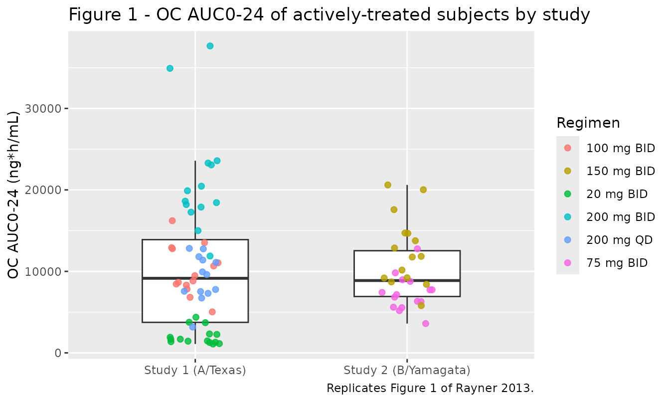
Replicates Figure 1 of Rayner 2013.

spread <- active |>
  dplyr::group_by(study) |>
  dplyr::summarise(
    median = median(AUC_OSELCARB),
    p05 = quantile(AUC_OSELCARB, 0.05),
    p95 = quantile(AUC_OSELCARB, 0.95),
    .groups = "drop"
  ) |>
  dplyr::mutate(fold_range = p95 / p05)

s1 <- spread[startsWith(spread$study, "Study 1"), ]
s2 <- spread[startsWith(spread$study, "Study 2"), ]

# Bounds below were measured across 1, 2, 4, 8 and 16 solver threads (the
# cohort differs per thread count; see the seeding comment above) and set
# outside the observed range. Do not tighten them back to a single run.
#
# Claim 1: "the median AUC0-24 values were closely similar". Study 1's active
# arms average 210 mg/day and study 2's 225 mg/day, so the medians agree
# structurally, but a 13-15 per arm draw moves each median by tens of percent.
# Realised median ratios 1.145 / 1.031 / 0.894 / 1.179 / 0.989 at 1 / 2 / 4 /
# 8 / 16 threads, i.e. within 18%. A factor-of-2 bound still breaks on a
# mis-transcribed dose, clearance or unit, all of which move the ratio far
# more than the draw does.
stopifnot(abs(log(s1$median / s2$median)) < log(2))

# Claim 2: "a wider range of exposures for subjects in study 1". Asserted as
# ABSOLUTE bounds implied by each study's dose range rather than as a race
# between two noisy statistics. Study 1 spans a 10-fold daily-dose range;
# study 2 spans only 2-fold, so nearly all of study 2's spread is IIV.
# Realised study-1 fold ranges 22.73 / 18.09 / 22.68 / 21.26 / 21.85 and
# study-2 fold ranges 3.61 / 3.54 / 3.44 / 4.96 / 4.06 at 1 / 2 / 4 / 8 / 16
# threads. The bounds below sit outside both ranges and still separate the two
# studies by more than a factor of two.
stopifnot(s1$fold_range > 8, s2$fold_range < 8)

spread |>
  dplyr::transmute(
    Study = study,
    `Median (ng*h/mL)` = round(median),
    `5th percentile` = round(p05),
    `95th percentile` = round(p95),
    `95th / 5th` = round(fold_range, 2)
  ) |>
  knitr::kable(caption = "Figure 1 summary: similar medians, wider spread in study 1.")

Figure 1 summary: similar medians, wider spread in study 1.

Study	Median (ng*h/mL)	5th percentile	95th percentile	95th / 5th
Study 1 (A/Texas)	9151	1291	23362	18.09
Study 2 (B/Yamagata)	8875	5346	18920	3.54

Figures 2A and 3A – composite symptom score AUC by exposure group

Figures 2A and 3A show the observed composite symptom score AUC by exposure group (2A) and by exposure group crossed with IC50 (3A). The packaged model predicts the group means those panels summarise.

pred_aucsc <- cohort |>
  dplyr::mutate(time = 0, evid = 0L, amt = NA_real_) |>
  (\(d) rxode2::rxSolve(
    ui$symptomscore, d,
    keep = c("treatment", "study"), returnType = "data.frame"
  ))() |>
  dplyr::mutate(
    Group = dplyr::case_when(
      aucHigh == 1 ~ "> 14,497",
      aucMid == 1 ~ "> 1,495 to 14,497",
      TRUE ~ "<= 1,495"
    ),
    Group = factor(Group,
                   levels = c("<= 1,495", "> 1,495 to 14,497", "> 14,497"))
  )

ggplot(pred_aucsc, aes(Group, aucsc, colour = study)) +
  geom_point(position = position_dodge(width = 0.4), size = 2.2) +
  labs(
    x = "OC AUC0-24 group (ng*h/mL)",
    y = "Predicted composite symptom score AUC (score*day)",
    colour = NULL,
    title = "Figures 2A / 3A - symptom burden falls as OC exposure rises",
    caption = "Replicates Figures 2A and 3A of Rayner 2013."
  )

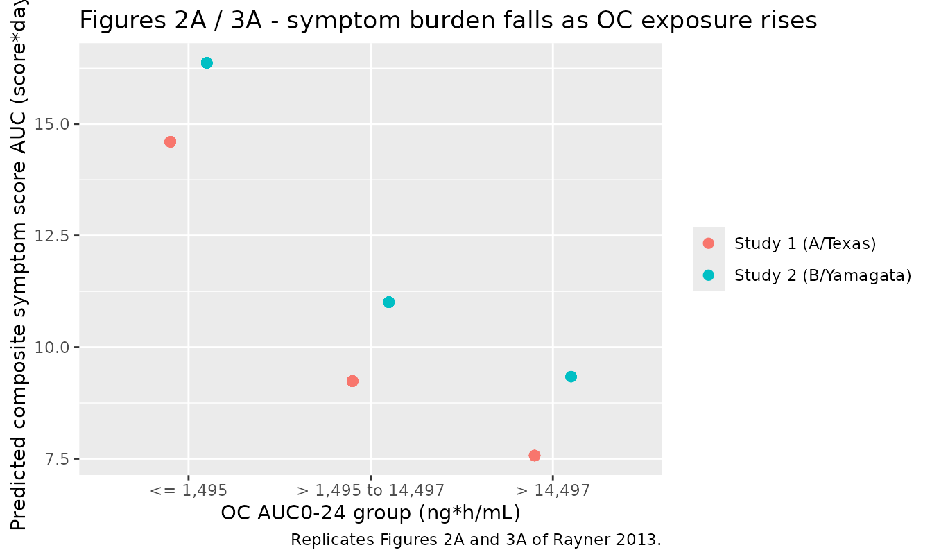
Replicates Figures 2A and 3A of Rayner 2013.

# The model is deterministic given the group AND the stratum, so each
# (Group, study) cell holds exactly one predicted value. Which cells the
# cohort populates depends on the draw, so the assertion is on the ORDERING
# WITHIN each study -- a property of the printed coefficients (-5.36 and -7.03
# are both negative and the second is larger in magnitude), not of the draw.
#
# Pooling the two studies before ordering would be wrong here: the strain
# effect is +1.77 score*day and the high-vs-middle contrast is only -1.67, so
# a strain-mixed group mean can invert the ordering purely from which study
# happened to supply each group's subjects.
cell <- pred_aucsc |>
  dplyr::group_by(study, Group) |>
  dplyr::summarise(
    aucsc = mean(aucsc), spread = diff(range(aucsc)), n = dplyr::n(),
    .groups = "drop"
  ) |>
  dplyr::arrange(study, Group)

stopifnot(
  nrow(cell) >= 4L,
  all(cell$n > 0),
  # Deterministic within a (study, Group) cell.
  all(cell$spread < 1e-12)
)
for (st in unique(cell$study)) {
  v <- cell$aucsc[cell$study == st]
  stopifnot(length(v) >= 2L, all(diff(v) < 0))
}

cell |>
  dplyr::transmute(
    Study = study,
    `OC AUC0-24 group (ng*h/mL)` = Group,
    `Subjects` = n,
    `Predicted AUCSC (score*day)` = round(aucsc, 2)
  ) |>
  knitr::kable(
    caption = paste(
      "Predicted composite symptom score AUC by exposure group and study.",
      "Monotone decreasing within each study."
    )
  )

Predicted composite symptom score AUC by exposure group and study. Monotone decreasing within each study.

Study	OC AUC0-24 group (ng*h/mL)	Subjects	Predicted AUCSC (score*day)
Study 1 (A/Texas)	<= 1,495	20	14.60
Study 1 (A/Texas)	> 1,495 to 14,497	35	9.24
Study 1 (A/Texas)	> 14,497	14	7.57
Study 2 (B/Yamagata)	<= 1,495	16	16.37
Study 2 (B/Yamagata)	> 1,495 to 14,497	25	11.01
Study 2 (B/Yamagata)	> 14,497	5	9.34

Figures 2B, 2C, 3B and 3C – time-to-event endpoints

Those four panels are stratified Kaplan-Meier curves. The packaged Cox models supply the relative hazard between strata, not an absolute survivor function, because a Cox fit leaves the baseline hazard unspecified (see Assumptions and deviations). What the models do reproduce is the hazard-ratio ladder that orders those curves.

hr_ladder <- dplyr::bind_rows(
  sim_six$symptomalleviation |>
    dplyr::mutate(Endpoint = "Alleviation of composite symptom score"),
  sim_six$shedding |>
    dplyr::mutate(Endpoint = "Cessation of viral shedding")
) |>
  dplyr::mutate(
    exposure = factor(exposure, levels = c("low", "middle", "high"))
  )

ggplot(hr_ladder, aes(exposure, hr, colour = strain, group = strain)) +
  geom_point(size = 2.6) +
  geom_line() +
  geom_hline(yintercept = 1, linetype = "dashed") +
  facet_wrap(~Endpoint) +
  scale_y_log10() +
  labs(
    x = "OC AUC0-24 group", y = "Hazard ratio vs low-exposure A/Texas",
    colour = "Infecting strain",
    title = "Figures 2B / 2C / 3B / 3C - hazard of the event rises with exposure",
    caption = "Replicates the hazard-ratio structure of Figures 2B, 2C, 3B and 3C of Rayner 2013."
  )

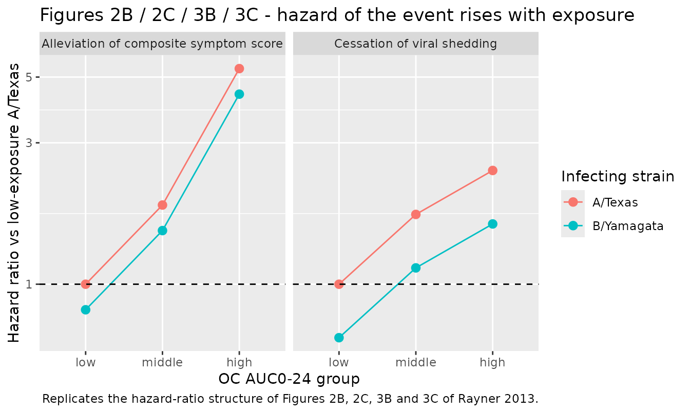
Hazard-ratio ladder underlying Figures 2B, 2C, 3B and 3C of Rayner 2013.

For reference, Table 4 gives the observed Kaplan-Meier percentiles those panels plot. They are reproduced here as published values, not as model predictions.

tibble::tribble(
  ~Endpoint, ~`OC AUC0-24 group (ng*h/mL)`, ~`Subjects`, ~`25th, 50th, 75th percentile (days)`,
  "Alleviation of symptoms", "<= 1,568",             "20 (18 placebo)", "2, 3.5, 4.5",
  "Alleviation of symptoms", "> 1,568 to <= 13,638", "30",              "1, 1.5, 3.5",
  "Alleviation of symptoms", "> 13,638",             "14",              "0.5, 0.75, 1.5",
  "Cessation of shedding",   "0",                    "22 (22 placebo)", "2.5, 4.75, 7",
  "Cessation of shedding",   "> 0 to <= 14,180",     "49",              "1, 2.5, 5.5",
  "Cessation of shedding",   "> 14,180",             "21",              "1, 2, 3"
) |>
  knitr::kable(
    caption = paste(
      "Rayner 2013 Table 4 (published Kaplan-Meier percentiles).",
      "These are observational summaries, not predictions of the packaged",
      "models, which carry no baseline hazard."
    )
  )

Rayner 2013 Table 4 (published Kaplan-Meier percentiles). These are observational summaries, not predictions of the packaged models, which carry no baseline hazard.

Endpoint	OC AUC0-24 group (ng*h/mL)	Subjects	25th, 50th, 75th percentile (days)
Alleviation of symptoms	<= 1,568	20 (18 placebo)	2, 3.5, 4.5
Alleviation of symptoms	> 1,568 to <= 13,638	30	1, 1.5, 3.5
Alleviation of symptoms	> 13,638	14	0.5, 0.75, 1.5
Cessation of shedding	0	22 (22 placebo)	2.5, 4.75, 7
Cessation of shedding	> 0 to <= 14,180	49	1, 2.5, 5.5
Cessation of shedding	> 14,180	21	1, 2, 3

Assumptions and deviations

• The Cox models carry no baseline hazard, by construction. A Cox proportional-hazards regression is semiparametric: the baseline hazard h0(t) is never estimated, so it is not an unreported parameter but a quantity the published fit does not contain. The two time-to-event model files therefore return the relative hazard hr and deliberately omit a survivor function; a user who wants absolute event times must supply h0(t). Table 4’s per-subgroup Kaplan-Meier percentiles were considered as a calibration target during extraction and rejected: fitting a Weibull baseline to the reference group’s printed 25th and 75th percentiles (2 and 4.5 days for symptom alleviation) and combining it with the published hazard ratio of 1.85 overpredicts the middle group’s own printed 25th and 50th percentiles by 46% and 53%. Shipping that baseline would have embedded a construction contradicting the paper’s own data, so the models stop at the relative hazard, which is exactly what the paper estimated.

• The linear-regression reference level is the Table 4 subgroup mean, not the Table 6 intercept. Table 6 prints only pairwise contrasts, and the multivariable intercept cannot be recovered exactly because that would require the IC50-by-exposure-group cross-tabulation the paper does not report. aucsc_int is set to 14.6 scoreday, the Table 4 observed mean of the lowest-exposure subgroup, whose identification is verified in validation section C above. Consequence: every contrast the model predicts is exact, while absolute aucsc predictions carry a bias no larger than the IC50 effect itself (1.77 scoreday), because 14.6 is marginal over the two strata whereas the model intercept is conditional on the influenza A stratum. Use d_aucsc, not aucsc, whenever an exactly-published quantity is needed.

• IC50 is a two-level categorical variable, not a slope. The paper states that IC50 was evaluated as a categorical variable because it took only two values (Table 2 footnote c). The models therefore apply the full effect to any IC50_NEURAMINIDASE above the printed 0.18 nM reference rather than interpolating. Supplying an intermediate IC50 is outside the model’s support.

• No IIV and no residual error. All three fits are subject-level regressions with one observation per subject, estimated in R 2.11.1 rather than NONMEM. The paper reports point estimates, confidence intervals, P values and AICc, and no variance component of any kind. No placeholder residual was invented and no observation endpoint is declared; the predictions fall out as derived variables, matching Nagy_2017_obiltoxaximab_survival and Lin_2020_glasdegib_decitabine.

• Non-significant covariate retained. The IC50 effect is not significant for any of the three endpoints (P = 0.257, 0.494 and 0.136) and every confidence interval spans the null. It is kept because the paper keeps it: IC50 is perfectly collinear with study identity, and demonstrating that it does not modify the exposure-response relationship is one of the paper’s two headline findings.

• Exposure covariate values are not packaged. AUC_OSELCARB is an input the user supplies. The individual post hoc values Rayner 2013 used are not published, so the cohort in this vignette regenerates them by simulating the studied regimens through modellib("Kamal_2013_oseltamivir") at the Table 1 covariate distributions. The reconstruction reproduces the one absolute exposure figure the paper states (about 6,000 ng*h/mL at 75 mg BID) to within 10%, but individual subjects are not the paper’s subjects.

• Cohort covariates assumed lognormal. Table 1 reports means and coefficients of variation but not distributional shapes. Weight, age and creatinine clearance are drawn lognormal with the tabulated mean and CV per study, which keeps every draw positive. Race was not used by any of the three models and is not simulated.

• The virtual cohort reconstructs the randomisation, not the dropouts. The arm sizes come from Table 1 and sum to the published 115 evaluable subjects. The endpoint-specific subsets (112, 64 and 92 subjects) reflect which subjects had evaluable data for each endpoint, which the paper does not break down by arm, so the cohort here is not filtered per endpoint.

• Endpoints the paper analysed but did not carry to a final model are not packaged. Viral titer AUC and peak viral titer were evaluated (Tables 2 and

  5. but the authors gave them no final multivariable model, judging the relationships not biologically plausible for an inoculation design in which peak titers occur before drug exposure builds up. There are consequently no parameter estimates to extract for them.