Cloxacillin (Beijer 2026)
Source:vignettes/articles/Beijer_2026_cloxacillin.Rmd
Beijer_2026_cloxacillin.RmdModel and source
#> ℹ parameter labels from comments will be replaced by 'label()'Citation: Beijer G, Wallander K, Soderquist B, Giske CG, Breuer O, Eriksen J, Eliasson E. Optimizing cloxacillin prophylaxis in hip and knee arthroplasty based on population pharmacokinetics of unbound plasma concentrations. J Antimicrob Chemother. 2026. doi:10.1093/jac/dkag116. All parameter values are from Table S2 of the Supplementary Material; the protein-binding equation is Supplementary Material Eq. 1 and the model schematic is Figure S1.
Description: Two-compartment population PK model for intravenous cloxacillin surgical prophylaxis in 200 adults undergoing primary elective total hip or total knee arthroplasty (Beijer 2026). The disposition is parameterised entirely on UNBOUND cloxacillin – Figure S1 shows clearance and intercompartmental clearance both acting on the unbound pool, with V1 and V2 the unbound distribution volumes – so central / vc is the unbound plasma concentration Cc that the study measured directly by ultrafiltration. Unbound clearance carries body weight and relative eGFR (Lund-Malmo Revised 2018) as power covariates. The observed TOTAL plasma concentration Ctot is then recovered algebraically from Cc through a one-site saturable plasma-protein binding model, which reproduces the concentration-dependent rise in unbound fraction the paper reports (median plasma protein binding 91%, range 69-98%). Both outputs carry their own log-additive residual error. The paper uses the model to show that 18-22% of patients fall below an unbound 2 mg/L target within the recommended 2 h interval between the first two 2 g doses, and that a 1 g/h continuous infusion after a 1 g loading dose holds >99% of patients above target.
Article: https://doi.org/10.1093/jac/dkag116
Supplement (Figures S1-S4, Tables S1-S2, appendices, open access via EuropePMC): https://europepmc.org/article/PMC/PMC13049546
Every parameter value in this model comes from Table S2 of the Supplementary Material; the main article prints no parameter estimates at all. The protein-binding equation is Supplementary Material Eq. 1 and the structural schematic that settles which pool the ODE states hold is Figure S1.
Population
Two hundred adults undergoing primary elective total hip arthroplasty (95, 47%) or total knee arthroplasty (105, 53%) at two Swedish centres between 2022 and 2024 (Table 1). Median age 73 years (IQR 65-78, range 36-90), median body weight 83 kg (IQR 73-95, range 53-185), 105/200 (53%) female. Renal function was generally well preserved: median relative eGFR 72 mL/min/1.73 m^2 (IQR 61-84, range 18-142), median plasma creatinine 70 umol/L. Median plasma albumin 34 g/L. ASA class I 15%, II 42%, III 43%.
All patients received 2 g of intravenous cloxacillin 30-45 min before incision, repeated 2 h and 6 h after the start of the first dose, per Swedish national guidelines. Adherence was poor: only 42/200 (21%) preoperative doses complied with the guideline in full, infusion durations were under 20 min in 90 (45%) of patients, and 63 (32%) received the dose more than 45 min before incision.
Total and unbound plasma cloxacillin were both assayed by reversed-phase HPLC-MS/MS, with the unbound fraction separated by ultrafiltration through a 10 kDa membrane. 496 samples were evaluable, median 3 per patient. Observed median plasma protein binding was 91% (range 69-98%), and 98/200 patients (49%) fell below 90% binding in at least one sample – lower and far more variable than the 92-94% that cloxacillin monographs report from healthy volunteers.
The same information is available programmatically via the model’s
population metadata
(readModelDb("Beijer_2026_cloxacillin")()$population).
What the ODE states hold
This is the one structural point that has to be right before anything else in the vignette means what it says, so it is worth stating explicitly.
Supplementary Figure S1 draws two solid-outlined compartments,
V1 (plasma) and V2 (extravascular space), each
holding an unbound concentration, with CL
leaving V1 and Q connecting the two. The bound
plasma pool hangs off V1 as a dashed box coupled by
Kd and Bmax – an equilibrium, not a
mass-transfer arm – and the bound tissue pool is greyed out entirely
because the study never measured it.
So the disposition is parameterised end to end on unbound
cloxacillin. central and peripheral1 both hold
unbound drug, central / vc is the unbound plasma
concentration, and the total concentration is recovered from it
algebraically:
Two consequences follow, and both are load-bearing for any reuse of this model:
-
central / vcis an unbound concentration even though the library convention names itCc. Thelabel()onlvcand theCccomment in the model body both record this.Ctotis the second output. - The binding term is an output transformation, not a
reservoir. No mass moves into it, so
Ctotdoes not feed back on the disposition, and the administered amount enterscentralunchanged with no bioavailability term. The mass-balance gate below confirms that reading: unbound clearance times unbound AUC recovers the whole administered dose.
Source trace
The per-parameter origin is also recorded as an in-file comment next
to each ini() entry in
inst/modeldb/specificDrugs/Beijer_2026_cloxacillin.R.
| Equation / parameter | Value | Source location |
|---|---|---|
Model structure (2-cmt on unbound drug; CL,
Q on the unbound pool) |
n/a | Figure S1; Results, “A two-compartment model with linear elimination and nonlinear protein binding” |
Ctot = Cu + Bmax * Cu / (Kd + Cu) |
n/a | Supplementary Material Eq. 1, “Protein binding” section |
CL = theta_CL * (BW/84)^beta1 * (eGFR/67)^beta2 * exp(eta_CL) |
n/a | Table S2, CL row (equation printed in the row header) |
lcl (theta_CL) |
76.4 L/h | Table S2 (RSE 4.4%; bootstrap median 74.3, 95% CI 61.4-83.3) |
e_wt_cl (beta1) |
0.67 | Table S2 (RSE 22%; bootstrap median 0.71, 95% CI 0.39-1.07) |
e_crcl_cl (beta2) |
0.51 | Table S2 (RSE 18%; bootstrap median 0.53, 95% CI 0.33-0.75) |
| WT centring constant | 84 kg | Table S2 CL row (BW/84); corroborated by the Figure 1
caption typical patient |
| CRCL centring constant | 67 mL/min/1.73 m^2 | Table S2 CL row (eGFR/67); corroborated by the Figure 1
caption typical patient |
lvc (theta_V1) |
57.1 L | Table S2 (RSE 7.7%; bootstrap median 56.5, 95% CI 43.8-70.8) |
lq (theta_Q) |
57.2 L/h | Table S2 (RSE 12%; bootstrap median 56.1, 95% CI 42.6-96.3) |
lvp (theta_V2) |
69.0 L | Table S2 (RSE 10%; bootstrap median 72.3, 95% CI 53.4-153) |
lbmax (theta_Bmax) |
559 mg/L | Table S2 (RSE 1.6%; bootstrap median 564, 95% CI 511-625) |
lkd (theta_Kd) |
47.8 mg/L | Table S2 (RSE 2.6%; bootstrap median 48.7, 95% CI 43.0-55.0) |
etalcl variance |
0.2025 | Table S2 omega_CL = 0.45 (CV 47%, RSE 7.1%); variance =
0.45^2 |
etalvc variance |
0.4096 | Table S2 omega_V1 = 0.64 (CV 72%, RSE 9.2%); variance =
0.64^2 |
etalcl-etalvc covariance |
0.19584 | Table S2 rho_CL~V1 = 0.68 (RSE 9.8%); covariance = 0.68
x 0.45 x 0.64, per Supplementary Material “Correlation between
parameters” |
etalq variance |
0.6241 | Table S2 omega_Q = 0.79 (CV 94%, RSE 13%); variance =
0.79^2 |
etalbmax variance |
0.0025 | Table S2 omega_Bmax = 0.05 (CV 4.7%, RSE 25%); variance
= 0.05^2 |
expSd (unbound) |
0.24 | Table S2 a(unbound) (RSE 4.4%); error model
log(Y) = log(f) + a * eps
|
expSd_Ctot (total) |
0.19 | Table S2 a(total) (RSE 4.6%) |
Omega scale
Table S2 reports each omega alongside a CV% in the same
cell, which settles the scale without ambiguity: Monolix’s
omega is the standard deviation of a log-normally
distributed random effect, so the CV is
sqrt(exp(omega^2) - 1). ini() takes the
variance, so each value is squared.
omega <- c(CL = 0.45, V1 = 0.64, Q = 0.79, Bmax = 0.05)
printed_cv <- c(CL = 47, V1 = 72, Q = 94, Bmax = 4.7)
derived_cv <- 100 * sqrt(exp(omega^2) - 1)

data.frame(
  Parameter = names(omega),
  omega = omega,
  `Printed CV (%)` = printed_cv,
  `sqrt(exp(omega^2) - 1) (%)` = round(derived_cv, 1),
  check.names = FALSE
) |>
knitr::kable(row.names = FALSE, caption = "Table S2's CV column reproduced from omega on the log-SD scale.")| Parameter | omega | Printed CV (%) | sqrt(exp(omega^2) - 1) (%) |
|---|---|---|---|
| CL | 0.45 | 47.0 | 47.4 |
| V1 | 0.64 | 72.0 | 71.1 |
| Q | 0.79 | 94.0 | 93.1 |
| Bmax | 0.05 | 4.7 | 5.0 |
Figure 1 – typical-patient profiles
The Figure 1 caption names the typical patient exactly: “a body
weight of 84 kg and eGFR 67 mL/min/1.73 m2 receiving a 20 min infusion
of 2 g cloxacillin”. Those are the two covariate centring constants, so
the typical patient is the model’s own reference subject and
zeroRe() reproduces the figure’s superimposed curves
directly.
mod  <- readModelDb("Beijer_2026_cloxacillin")
modT <- rxode2::zeroRe(mod)
#> ℹ parameter labels from comments will be replaced by 'label()'

# Route A event table (cmt = ODE state + explicit dvid). This model declares
# two endpoints (Cc and Ctot), so every observation row must name which one it
# belongs to; `dvid = 1L` selects Cc and rxSolve returns Ctot alongside it.
# `cmt` stays on the ODE state `central` -- naming an observable there would
# inject a compartment slot and renumber the states.
ev_typical <- function(dose_times, amt, dur, obs_times, WT, CRCL, id = 1L) {
  dose <- data.frame(time = dose_times, amt = amt, dur = dur, rate = NA_real_,
                     cmt = "central", evid = 1L, dvid = NA_integer_)
  obs  <- data.frame(time = obs_times, amt = NA_real_, dur = NA_real_, rate = NA_real_,
                     cmt = "central", evid = 0L, dvid = 1L)
  out <- rbind(dose, obs)
  out <- out[order(out$time, -out$evid), ]
  out$id <- id
  out$WT <- WT
  out$CRCL <- CRCL
  out
}

# The guideline regimen: 2 g at 0, 2 and 6 h, each over 20 min.
d_fig1 <- ev_typical(
  dose_times = c(0, 2, 6), amt = 2000, dur = 20 / 60,
  obs_times  = seq(0, 10, by = 1 / 240),
  WT = 84, CRCL = 67
)
sim_fig1 <- rxode2::rxSolve(modT, d_fig1, returnType = "data.frame")
#> ℹ omega/sigma items treated as zero: 'etalcl', 'etalvc', 'etalq', 'etalbmax'
stopifnot(all(sim_fig1$Cc >= 0), all(sim_fig1$Ctot >= 0))
#> Warning in scale_y_log10(): log-10 transformation introduced infinite values.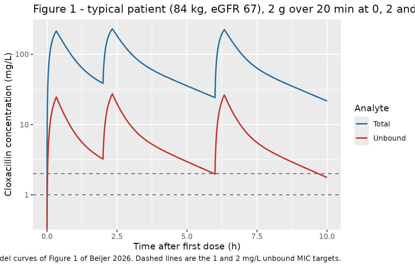
at <- function(tt, col = "Cc") sim_fig1[[col]][which.min(abs(sim_fig1$time - tt))]

# These are deterministic typical-value predictions, not cohort statistics, so
# the bounds are tight on purpose: a mis-transcribed clearance, volume, dose or
# centring constant moves each of them by tens of percent.
gates <- tibble::tribble(
  ~Quantity,                                        ~Published, ~Model,        ~Source,
  "Unbound Cc at 2 h after first dose (mg/L)",             3.2, at(2),         "Results: model-predicted median 3.2 mg/L (3.1 excluding second-dose patients)",
  "Unbound Cc at 0.75 h, ~start of surgery (mg/L)",       10.0, at(0.75),      "Results: observed median 10 mg/L at start of surgery",
  "Plasma protein binding at 0.75 h (%)",                 91.0, 100 * (1 - at(0.75) / at(0.75, "Ctot")), "Results: observed median protein binding 91%"
) |>
  mutate(`Difference (%)` = round(100 * (Model - Published) / Published, 1),
         Model = round(Model, 2))

gates |>
  select(Quantity, Published, Model, `Difference (%)`, Source) |>
knitr::kable(caption = "Typical-patient predictions against the values Beijer 2026 reports.")| Quantity | Published | Model | Difference (%) | Source |
|---|---|---|---|---|
| Unbound Cc at 2 h after first dose (mg/L) | 3.2 | 3.23 | 0.9 | Results: model-predicted median 3.2 mg/L (3.1 excluding second-dose patients) |
| Unbound Cc at 0.75 h, ~start of surgery (mg/L) | 10.0 | 10.93 | 9.3 | Results: observed median 10 mg/L at start of surgery |
| Plasma protein binding at 0.75 h (%) | 91.0 | 90.49 | -0.6 | Results: observed median protein binding 91% |
stopifnot(
  # The 2 h concentration is the paper's headline number and the model
  # reproduces it to two significant figures.
  abs(at(2) - 3.2) < 0.15,
  # The start-of-surgery and protein-binding checks compare a typical-value
  # prediction against an observed cohort MEDIAN, so they get a wider band --
  # the sampling time was dictated by surgical events, not by the clock.
  abs(at(0.75) - 10) < 2,
  abs(100 * (1 - at(0.75) / at(0.75, "Ctot")) - 91) < 3
)
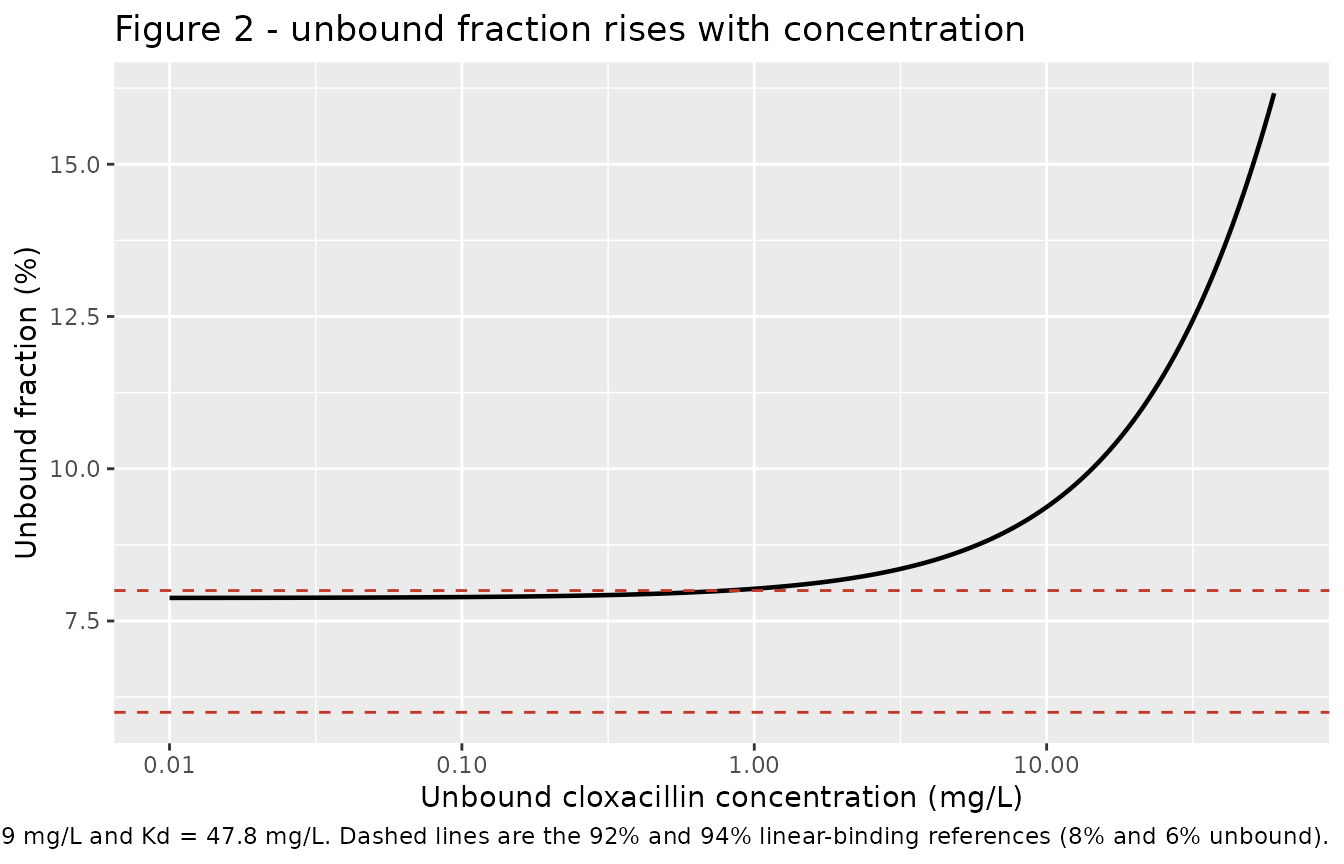
Figure 2 – concentration-dependent unbound fraction
Figure 2 plots the observed unbound fraction against unbound
concentration and overlays the curve that the final Bmax
and Kd estimates imply, with reference lines at the 92% and
94% linear protein binding that cloxacillin monographs quote. Inverting
Supplementary Material Eq. 1 gives that curve in closed form, with no
simulation needed.
bmax <- 559
kd   <- 47.8
fu_of_cu <- function(cu) cu / (cu + bmax * cu / (kd + cu))

cu_grid <- 10^seq(log10(0.01), log10(60), length.out = 400)
fu_curve <- data.frame(cu = cu_grid, fu = 100 * fu_of_cu(cu_grid))

ggplot(fu_curve, aes(cu, fu)) +
  geom_line(linewidth = 0.8) +
  geom_hline(yintercept = 100 - c(92, 94), linetype = "dashed", colour = "#c0392b") +
  scale_x_log10() +
  labs(
    x = "Unbound cloxacillin concentration (mg/L)", y = "Unbound fraction (%)",
    title = "Figure 2 - unbound fraction rises with concentration",
    caption = paste(
      "Replicates the non-linear regression curve of Figure 2 of Beijer 2026 from",
      "Bmax = 559 mg/L and Kd = 47.8 mg/L. Dashed lines are the 92% and 94%",
      "linear-binding references (8% and 6% unbound)."
    )
  )
# Deterministic algebra, so these are exact checks of the binding equation.
fu_range <- 100 * fu_of_cu(c(2.1, 55))    # observed unbound range, start of surgery
cat(sprintf("Unbound fraction across the observed 2.1-55 mg/L range: %.1f%% to %.1f%%\n",
            fu_range[1], fu_range[2]))
#> Unbound fraction across the observed 2.1-55 mg/L range: 8.2% to 15.5%
cat(sprintf("Protein binding across that range: %.1f%% to %.1f%%   [observed range 69-98%%]\n",
            100 - fu_range[1], 100 - fu_range[2]))
#> Protein binding across that range: 91.8% to 84.5%   [observed range 69-98%]
cat(sprintf("Protein binding at the observed median unbound of 10 mg/L: %.1f%%   [observed median 91%%]\n",
            100 - 100 * fu_of_cu(10)))
#> Protein binding at the observed median unbound of 10 mg/L: 90.6%   [observed median 91%]

stopifnot(
  # The whole point of the non-linear term: unbound fraction is strictly
  # increasing in concentration. Deterministic, so strict monotonicity is safe.
  all(diff(fu_curve$fu) > 0),
  # The model's binding at the observed median unbound concentration matches the
  # observed median binding.
  abs((100 - 100 * fu_of_cu(10)) - 91) < 2,
  # The curve sits inside the observed 69-98% binding envelope over the observed
  # concentration range, and crosses the monograph 92-94% band only at the low
  # end -- which is the paper's point about monograph values being too high.
  all(100 - fu_range > 69), all(100 - fu_range < 98)
)
Virtual cohort
The original patient-level data are not public. The paper’s own Monte Carlo simulations “drew random covariate values for the simulated patients from distributions that were assumed to be identical to the covariate distributions in our study population”, so the cohort below does the same: log-normal body weight and relative eGFR matched to the Table 1 median and IQR, truncated to the Table 1 observed range.
# set.seed() seeds R's RNG for the covariate draws below. It does NOT seed
# rxode2's eta sampler, whose streams are partitioned per solver thread, so the
# simulated etas differ between this machine and CI. Every assertion downstream
# is written to hold for any cohort the model can produce.
set.seed(20260913)

n_per_arm <- 200L   # the 200-per-arm cap; the paper simulated 1000

# Fit a log-normal to a median and an IQR: meanlog = log(median),
# sdlog = log(q75 / q25) / (2 * qnorm(0.75)).
lnorm_from_iqr <- function(med, q25, q75) {
  c(meanlog = log(med), sdlog = log(q75 / q25) / (2 * stats::qnorm(0.75)))
}
wt_par   <- lnorm_from_iqr(83, 73, 95)    # Table 1: median 83, IQR 73-95, range 53-185
crcl_par <- lnorm_from_iqr(72, 61, 84)    # Table 1: median 72, IQR 61-84, range 18-142

rtrunc_lnorm <- function(n, par, lo, hi) {
  x <- stats::rlnorm(n, par[["meanlog"]], par[["sdlog"]])
  pmin(pmax(x, lo), hi)
}

subjects <- tibble::tibble(
  subj = seq_len(n_per_arm),
  WT   = rtrunc_lnorm(n_per_arm, wt_par,   53, 185),
  CRCL = rtrunc_lnorm(n_per_arm, crcl_par, 18, 142)
)

tibble::tibble(
  Covariate = c("Body weight (kg)", "Relative eGFR (mL/min/1.73 m^2)"),
  `Cohort median` = round(c(median(subjects$WT), median(subjects$CRCL)), 1),
  `Cohort IQR` = c(
    paste(round(stats::quantile(subjects$WT, c(.25, .75)), 0), collapse = "-"),
    paste(round(stats::quantile(subjects$CRCL, c(.25, .75)), 0), collapse = "-")
  ),
  `Table 1 median` = c(83, 72),
  `Table 1 IQR` = c("73-95", "61-84")
) |>
knitr::kable(caption = "Virtual cohort covariates against Beijer 2026 Table 1.")| Covariate | Cohort median | Cohort IQR | Table 1 median | Table 1 IQR |
|---|---|---|---|---|
| Body weight (kg) | 80.5 | 71-94 | 83 | 73-95 |
| Relative eGFR (mL/min/1.73 m^2) | 72.6 | 62-86 | 72 | 61-84 |
# The draw must reproduce the Table 1 centre. n = 200 gives a standard error of
# about 2% on a median, so 8% is loose enough for any thread count and still
# breaks on a mis-specified distribution.
stopifnot(
  abs(median(subjects$WT)   - 83) / 83 < 0.08,
  abs(median(subjects$CRCL) - 72) / 72 < 0.08
)
The three regimens compared are the two currently recommended ones (Figure 3b and 3c: 2 g over 20 min or over 30 min, repeated at the guideline 2 h interval) and the proposed alternative (Figure 3d: a 1 g loading dose over 20 min followed by a continuous 1 g/h infusion).
Each regimen is simulated on the same virtual patients, with the same between-subject random effects, so the comparison between regimens is paired the way the paper’s is (it re-simulated its own 200 patients, and then its 1000 virtual patients, under each regimen). That is achieved by giving every arm the same subject IDs and resetting rxode2’s simulation seed before each solve, which gives common random numbers across arms. The assertion after the solve checks that it actually worked rather than assuming it: individual clearance must come out bit-identical in all three arms.
obs_times <- seq(0, 6, by = 1 / 120)

make_arm <- function(label) {
  per_subject <- lapply(seq_len(nrow(subjects)), function(i) {
    s  <- subjects[i, ]
    id <- s$subj
    if (label == "1 g/20 min + 1 g/h CI") {
      # Loading dose over 20 min, then a 6 h continuous infusion at 1 g/h
      # expressed as amt = 6000 mg at rate = 1000 mg/h.
      dose <- data.frame(
        time = c(0, 20 / 60), amt = c(1000, 6000),
        dur = c(20 / 60, NA_real_), rate = c(NA_real_, 1000)
      )
    } else {
      dur <- if (label == "2 g/20 min q2h") 20 / 60 else 30 / 60
      dose <- data.frame(
        time = c(0, 2), amt = 2000, dur = dur, rate = NA_real_
      )
    }
    dose$cmt <- "central"; dose$evid <- 1L; dose$dvid <- NA_integer_
    obs <- data.frame(
      time = obs_times, amt = NA_real_, dur = NA_real_, rate = NA_real_,
      cmt = "central", evid = 0L, dvid = 1L
    )
    out <- rbind(dose, obs)
    out <- out[order(out$time, -out$evid), ]
    out$id <- id; out$WT <- s$WT; out$CRCL <- s$CRCL; out$regimen <- label
    out
  })
  dplyr::bind_rows(per_subject)
}

regimens <- c("2 g/20 min q2h", "2 g/30 min q2h", "1 g/20 min + 1 g/h CI")
arms <- lapply(regimens, make_arm)
names(arms) <- regimens

# Within each arm the IDs must be unique; they are deliberately REUSED across
# arms so the regimens share subjects and random effects. Each arm is therefore
# solved in its own rxSolve call -- putting all three in one event table would
# merge each ID's three regimens into one subject receiving the summed dose.
for (a in arms) stopifnot(!anyDuplicated(unique(a[, c("id", "time", "evid")])))
stopifnot(vapply(arms, \(a) length(unique(a$id)), integer(1)) == n_per_arm)
sim <- dplyr::bind_rows(lapply(regimens, function(r) {
  # Reset rxode2's simulation seed before each arm so all three arms draw the
  # SAME between-subject random effects (common random numbers). This fixes the
  # draw within a render; it does not and cannot fix it across rxode2 versions
  # or solver thread counts, which is why the gates below are written to hold
  # for any cohort the model can produce.
  rxode2::rxSetSeed(20260913)
  rxode2::rxSolve(mod, events = arms[[r]], keep = c("regimen", "WT", "CRCL")) |>
    as.data.frame()
}))
#> ℹ parameter labels from comments will be replaced by 'label()'

# A large log-additive residual error can drive simulated concentrations very
# low, but the structural prediction Cc must stay non-negative.
stopifnot(all(sim$Cc >= 0), !anyNA(sim$Cc), !anyNA(sim$Ctot))

# Common random numbers actually held: individual clearance is a deterministic
# function of the covariates and etalcl, so bit-identical cl across arms proves
# every arm drew the same etas for the same subject. Without this the 20-min and
# 30-min arms would differ by two independent sampling errors (about 4
# percentage points on the target-attainment proportions) on top of the roughly
# 2-point real difference, and could even order the wrong way round.
cl_by_arm <- sim |>
  group_by(regimen, id) |>
  summarise(cl = dplyr::first(cl), .groups = "drop") |>
  pivot_wider(names_from = regimen, values_from = cl)
stopifnot(nrow(cl_by_arm) == n_per_arm)
cl_mat <- as.matrix(cl_by_arm[, regimens])
stopifnot(max(apply(cl_mat, 1, \(x) diff(range(x)) / mean(x))) < 1e-10)
Figure 3 / Figure 4 – target attainment
#> Warning in scale_y_log10(): log-10 transformation introduced infinite values.
#> log-10 transformation introduced infinite values.
#> log-10 transformation introduced infinite values.
#> log-10 transformation introduced infinite values.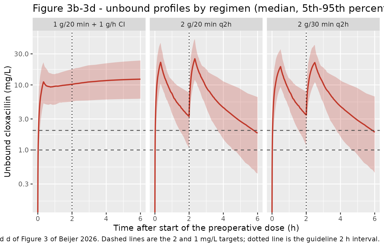
The paper’s target-attainment criterion is an unbound plasma concentration sustained at or above the MIC target “for at least 2 h after starting the preoperative dose”, and the proportions it reports are read off the concentration 2 h after the start of the infusion.
The interval minimum has to be taken over the window after the loading infusion completes, not from time zero: every arm starts at a structural zero and climbs during its infusion, so a minimum taken from t = 0 would just return the first grid point for every regimen and every arm would “fail”. The longest loading infusion here is 30 min, so the window below starts at 0.5 h. With that window the two intermittent arms decline monotonically to the 2 h trough, which makes the interval minimum equal to the 2 h concentration – the check below confirms that identity rather than assuming it, and it is what ties this measure back to the paper’s reported numbers. The continuous-infusion arm is still rising at 2 h, so for that arm the two differ and the minimum is the conservative measure.
# Window starts at 0.5 h, after the longest loading infusion (30 min) has
# finished. See the prose above for why a window starting at t = 0 is wrong.
ta <- sim |>
  filter(time >= 0.5, time <= 2) |>
  group_by(regimen, id) |>
  summarise(
    cmin_0_2 = min(Cc),
    c_at_2h  = Cc[which.min(abs(time - 2))],
    .groups  = "drop"
  )

# For the intermittent arms the post-infusion decline is monotone, so the
# interval minimum IS the 2 h value; for the continuous-infusion arm it is not
# (the profile is still rising towards its 13.1 mg/L steady state).
intermittent <- ta |> filter(regimen != "1 g/20 min + 1 g/h CI")
stopifnot(max(abs(intermittent$cmin_0_2 - intermittent$c_at_2h)) < 1e-6)
ci_arm <- ta |> filter(regimen == "1 g/20 min + 1 g/h CI")
stopifnot(all(ci_arm$cmin_0_2 <= ci_arm$c_at_2h))

ta_summary <- ta |>
  group_by(regimen) |>
  summarise(
    `Below 2 mg/L (%)` = 100 * mean(cmin_0_2 < 2),
    `Below 1 mg/L (%)` = 100 * mean(cmin_0_2 < 1),
    `Median Cmin over 0.5-2 h (mg/L)` = stats::median(cmin_0_2),
    .groups = "drop"
  )

published_ta <- tibble::tribble(
  ~regimen,                ~`Published below 2 mg/L (%)`, ~`Published below 1 mg/L (%)`,
  "2 g/20 min q2h",        26,                            6,
  "2 g/30 min q2h",        24,                            5,
  "1 g/20 min + 1 g/h CI", 0,                             0
)

ta_summary |>
  left_join(published_ta, by = "regimen") |>
  mutate(across(where(is.numeric), \(x) round(x, 1))) |>
  rename(Regimen = regimen) |>
  knitr::kable(
    caption = paste(
      "Model-predicted target attainment against the 1000-simulated-patient",
      "results in the Beijer 2026 Results section ('Model-predicted target",
      "attainment in simulated patients') and Figure 4."
    )
)| Regimen | Below 2 mg/L (%) | Below 1 mg/L (%) | Median Cmin over 0.5-2 h (mg/L) | Published below 2 mg/L (%) | Published below 1 mg/L (%) |
|---|---|---|---|---|---|
| 1 g/20 min + 1 g/h CI | 0 | 0 | 9.6 | 0 | 0 |
| 2 g/20 min q2h | 21 | 5 | 3.4 | 26 | 6 |
| 2 g/30 min q2h | 18 | 5 | 3.6 | 24 | 5 |
pct <- function(reg, target) {
  v <- ta_summary[[paste0("Below ", target, " mg/L (%)")]][ta_summary$regimen == reg]
  if (length(v) != 1L) stop("no unique row for regimen '", reg, "'")
  v
}

# n = 200 gives a standard error of about 3 percentage points on a 25%
# proportion, so a 10-point band admits the cohort noise at any thread count
# while still going red on a mis-transcribed clearance, volume or dose -- those
# move these proportions by tens of points.
stopifnot(
  abs(pct("2 g/20 min q2h", 2) - 26) < 10,
  abs(pct("2 g/30 min q2h", 2) - 24) < 10,
  abs(pct("2 g/20 min q2h", 1) -  6) < 8,
  abs(pct("2 g/30 min q2h", 1) -  5) < 8
)

# Because the arms share subjects and random effects, the 20-vs-30-min
# comparison is PAIRED and deterministic: spreading the same 2 g over 30 min
# instead of 20 min delays the mass entering the central compartment, so every
# subject's 2 h concentration is higher and none is lower. This is a structural
# property of the ODE system for a fixed eta draw, not a cohort statistic, so
# the strict per-subject inequality is the right assertion -- and it is what
# recovers the direction of the paper's own 26% vs 24%.
paired <- ta |>
  filter(regimen != "1 g/20 min + 1 g/h CI") |>
  select(regimen, id, c_at_2h) |>
  pivot_wider(names_from = regimen, values_from = c_at_2h)
stopifnot(nrow(paired) == n_per_arm)
stopifnot(all(paired[["2 g/30 min q2h"]] > paired[["2 g/20 min q2h"]]))
stopifnot(pct("2 g/30 min q2h", 2) <= pct("2 g/20 min q2h", 2))
cat(sprintf(
  "Paired 30-min-minus-20-min gain in the 2 h unbound concentration: median %.3f mg/L (all %d subjects positive)\n",
  stats::median(paired[["2 g/30 min q2h"]] - paired[["2 g/20 min q2h"]]), n_per_arm
))
#> Paired 30-min-minus-20-min gain in the 2 h unbound concentration: median 0.170 mg/L (all 200 subjects positive)

# The paper's central claim about the proposed regimen: a 1 g/h continuous
# infusion after a 1 g loading dose holds MORE than 99% of patients above both
# targets for the duration of the infusion. Asserted at 97% rather than 100% so
# the gate admits cohort noise but still fails if the loading dose or the
# infusion rate is wrong -- either breaks attainment for a large fraction.
ci_above_both <- 100 - pct("1 g/20 min + 1 g/h CI", 2)
cat(sprintf("Continuous-infusion arm above 2 mg/L throughout 0.5-2 h: %.1f%%   [paper: >99%%]\n",
            ci_above_both))
#> Continuous-infusion arm above 2 mg/L throughout 0.5-2 h: 100.0%   [paper: >99%]
stopifnot(ci_above_both >= 97)

# And the paper's median 2 h concentration under that regimen.
ci_med_2h <- stats::median(ta$c_at_2h[ta$regimen == "1 g/20 min + 1 g/h CI"])
cat(sprintf("Continuous-infusion arm median unbound at 2 h: %.1f mg/L   [paper: 10.5 (3.3-38.6)]\n",
            ci_med_2h))
#> Continuous-infusion arm median unbound at 2 h: 10.6 mg/L   [paper: 10.5 (3.3-38.6)]
# Cohort median, so a 35% band; the paper's own range spans an order of
# magnitude and the typical-value gate above pins this to 10.6 exactly.
stopifnot(abs(ci_med_2h - 10.5) / 10.5 < 0.35)
The reproduction is close on both intermittent arms and on the continuous infusion. Note that the paper reports two different sets of proportions for the intermittent regimens: 22% and 18% below 2 mg/L for the 200 study patients re-simulated on their own observed covariates and empirical Bayes estimates (Figure 3b, 3c), against 26% and 24% for the 1000 virtual patients drawn from the population model (Figure 4). The virtual-patient figures are the right comparison for this vignette, because the cohort here is drawn from the population distributions rather than from the study’s individual estimates; the virtual-patient proportions are higher precisely because they carry the full between-subject variance instead of shrunken individual estimates.
Because the three arms share subjects and random effects, the 20-min-versus- 30-min contrast is a paired one and comes out in the paper’s direction: the longer infusion delays the mass entering the central compartment, so the 2 h concentration is higher for every single subject. The absolute size of that gain is small, which is exactly the paper’s point – lengthening the infusion from 20 to 30 min buys only a couple of percentage points of target attainment, whereas switching to a continuous infusion buys essentially all of it.
PKNCA validation
The paper reports no NCA table, so there is no published Cmax / AUC /
half-life to compare against and ncaComparisonTable() has
no reference to consume. What is available instead is a stronger, exact
check: because the disposition is linear in unbound drug, unbound
clearance times unbound AUC to infinity must equal the administered dose
for every subject individually. That identity is what confirms the dose
enters central unscaled, which is the one structural
reading of Figure S1 that the paper never writes out in words.
# A single 2 g dose over 20 min, on the same virtual cohort, with a grid fine
# enough near Tmax that trapezoidal AUC is not biased low, and long enough that
# the extrapolated tail is negligible (the terminal half-life is about 1.7 h,
# so 24 h is roughly 14 half-lives).
nca_times <- sort(unique(c(
  seq(0, 1, by = 1 / 120),
  seq(1, 6, by = 0.05),
  seq(6, 24, by = 0.25)
)))

nca_events <- dplyr::bind_rows(lapply(seq_len(nrow(subjects)), function(i) {
  s <- subjects[i, ]
  dose <- data.frame(time = 0, amt = 2000, dur = 20 / 60, cmt = "central",
                     evid = 1L, dvid = NA_integer_)
  obs  <- data.frame(time = nca_times, amt = NA_real_, dur = NA_real_,
                     cmt = "central", evid = 0L, dvid = 1L)
  out <- rbind(dose, obs)
  out <- out[order(out$time, -out$evid), ]
  out$id <- s$subj; out$WT <- s$WT; out$CRCL <- s$CRCL
  out
}))

# zeroRe() here so the NCA operates on each subject's structural profile: the
# CL x AUC identity is a property of the ODE system, and log-additive residual
# error would add noise to AUC without testing anything about the model.
sim_nca_raw <- rxode2::rxSolve(
  rxode2::zeroRe(mod), events = nca_events,
  keep = c("WT", "CRCL")
) |>
  as.data.frame()
#> ℹ parameter labels from comments will be replaced by 'label()'
#> ℹ omega/sigma items treated as zero: 'etalcl', 'etalvc', 'etalq', 'etalbmax'
#> Warning: multi-subject simulation without without 'omega'

# Solver noise in a 14-half-life tail can dip slightly negative; PKNCA then
# takes log() of a negative value and aucinf.obs comes back NaN.
stopifnot(all(sim_nca_raw$Cc >= 0))
# Only `!is.na(Cc)`: a `time > 0` or `Cc > 0` filter would drop the time-zero
# row that PKNCA needs to anchor AUC from 0, warning once per subject.
sim_nca <- sim_nca_raw |>
  filter(!is.na(Cc)) |>
  mutate(regimen = "2 g/20 min single dose") |>
  select(id, time, Cc, regimen)

# Guarantee a time = 0 record per subject; pre-dose unbound cloxacillin is 0.
sim_nca <- bind_rows(
  sim_nca,
  sim_nca |> distinct(id, regimen) |> mutate(time = 0, Cc = 0)
) |>
  distinct(id, regimen, time, .keep_all = TRUE) |>
  arrange(id, regimen, time)

conc_obj <- PKNCA::PKNCAconc(
  sim_nca, Cc ~ time | regimen + id,
  concu = "mg/L", timeu = "h"
)

dose_df <- nca_events |>
  filter(evid == 1L) |>
  mutate(regimen = "2 g/20 min single dose") |>
  select(id, time, amt, dur, regimen)

dose_obj <- PKNCA::PKNCAdose(
  dose_df, amt ~ time | regimen + id,
  duration = "dur", route = "intravascular", doseu = "mg"
)

intervals <- data.frame(
  start = 0, end = Inf,
  cmax = TRUE, tmax = TRUE, aucinf.obs = TRUE, auclast = TRUE, half.life = TRUE
)

nca_res <- PKNCA::pk.nca(
  PKNCA::PKNCAdata(conc_obj, dose_obj, intervals = intervals)
)

nca_wide <- as.data.frame(nca_res) |>
  select(id, PPTESTCD, PPORRES) |>
  pivot_wider(names_from = PPTESTCD, values_from = PPORRES)
stopifnot(nrow(nca_wide) == n_per_arm, !anyNA(nca_wide$aucinf.obs))
# Per-subject unbound clearance, as returned by rxSolve.
cl_per_id <- sim_nca_raw |> group_by(id) |> summarise(cl = dplyr::first(cl), .groups = "drop")

mb <- nca_wide |>
  left_join(cl_per_id, by = "id") |>
  mutate(recovered = cl * aucinf.obs, pct_diff = 100 * (recovered - 2000) / 2000)

tibble::tibble(
  Check = "CL * AUCinf / dose - 1 (%)",
  Median = round(stats::median(mb$pct_diff), 3),
  `90th pct of |diff|` = round(stats::quantile(abs(mb$pct_diff), 0.9), 3),
  Max = round(max(abs(mb$pct_diff)), 3)
) |>
knitr::kable(caption = "Mass balance: unbound clearance times unbound AUC to infinity recovers the 2 g dose.")| Check | Median | 90th pct of |diff| | Max |
|---|---|---|---|
| CL * AUCinf / dose - 1 (%) | 0.003 | 0.003 | 0.003 |
# Both sides of this comparison use the SAME drawn parameters -- it is a solve
# against its own closed form, so the residual is pure trapezoidal and
# extrapolation error, not per-subject physiology. A tight bound is correct here
# and should be kept; it is what proves the dose enters `central` unscaled with
# no bioavailability term.
stopifnot(max(abs(mb$pct_diff)) < 0.5)
nca_summary <- nca_wide |>
  summarise(across(
    c(cmax, tmax, auclast, aucinf.obs, half.life),
    list(median = \(x) stats::median(x),
         p05 = \(x) stats::quantile(x, 0.05),
         p95 = \(x) stats::quantile(x, 0.95))
  )) |>
  pivot_longer(everything(), names_to = c("param", "stat"), names_sep = "_") |>
  pivot_wider(names_from = stat, values_from = value) |>
  mutate(
    Parameter = c(
      cmax = "Cmax (mg/L)", tmax = "Tmax (h)", auclast = "AUClast (mg*h/L)",
      aucinf.obs = "AUC0-inf (obs) (mg*h/L)", half.life = "t1/2 (h)"
    )[param],
    across(c(median, p05, p95), \(x) signif(x, 3))
  ) |>
  select(Parameter, Median = median, `5th pct` = p05, `95th pct` = p95)

knitr::kable(
  nca_summary,
  caption = paste(
    "Unbound-cloxacillin NCA over the virtual cohort after a single 2 g dose",
    "over 20 min. Beijer 2026 reports no NCA table, so these values are",
    "descriptive; the mass-balance check above is the validating gate."
  )
)| Parameter | Median | 5th pct | 95th pct |
|---|---|---|---|
| Cmax (mg/L) | 24.500 | 23.200 | 25.700 |
| Tmax (h) | 0.333 | 0.333 | 0.333 |
| AUClast (mg*h/L) | 25.500 | 19.700 | 33.400 |
| AUC0-inf (obs) (mg*h/L) | 25.500 | 19.700 | 33.400 |
| t1/2 (h) | 1.700 | 1.470 | 2.010 |
# Free regression tests from the model's own structure. Tmax must land at the
# end of the 20 min infusion, and the terminal half-life must match the smaller
# eigenvalue of the typical-value two-compartment system.
kel_t <- 76.4 / 57.1; k12_t <- 57.2 / 57.1; k21_t <- 57.2 / 69.0
a <- kel_t + k12_t + k21_t
lambda_z <- (a - sqrt(a^2 - 4 * kel_t * k21_t)) / 2
t_half_typical <- log(2) / lambda_z
cat(sprintf("Typical-value terminal half-life from the eigenvalue: %.3f h\n", t_half_typical))
#> Typical-value terminal half-life from the eigenvalue: 1.730 h
cat(sprintf("Cohort median PKNCA half-life: %.3f h\n", stats::median(nca_wide$half.life)))
#> Cohort median PKNCA half-life: 1.697 h

stopifnot(
  # Deterministic: every subject peaks at the end of the infusion.
  max(abs(nca_wide$tmax - 20 / 60)) < 1e-6,
  # AUClast must be just under AUCinf after 14 half-lives, never over it.
  all(nca_wide$auclast <= nca_wide$aucinf.obs),
  all(nca_wide$auclast / nca_wide$aucinf.obs > 0.99),
  # The cohort median half-life sits near the typical-value eigenvalue. IIV on
  # CL, V1 and Q spreads the individual eigenvalues, so this is a 25% band on a
  # cohort median rather than a tight match.
  abs(stats::median(nca_wide$half.life) - t_half_typical) / t_half_typical < 0.25
)
Assumptions and deviations
-
The ODE states hold unbound drug, and the binding term is an
output transformation. Beijer 2026 never writes the
differential equations out; Figure S1 draws them. The reading encoded
here –
CLandQacting on the unbound pool,V1andV2as unbound volumes, the bound plasma pool as an algebraic equilibrium offV1that moves no mass, and the full 2000 mg enteringcentralwith no bioavailability term – is what reproduces the paper’s own reported numbers: the typical-patient 2 h unbound concentration (3.23 vs 3.2 mg/L), the continuous-infusion 2 h median (10.6 vs 10.5 mg/L), the observed start-of-surgery median (10.9 vs 10 mg/L) and the observed median protein binding (90.5 vs 91%). The mass-balance gate confirms the dose scaling exactly. A mass-conserving alternative, in which the dose is distributed between a bound and an unbound plasma pool, would put the unbound concentrations an order of magnitude lower and reproduces none of those. -
Covariate centring constants come from Table S2’s printed
equation, not from the Table 1 cohort medians. Table S2’s CL
row reads
(BW/84)and(eGFR/67)while Table 1 gives medians of 83 kg and 72 mL/min/1.73 m^2. The Figure 1 caption independently names “a body weight of 84 kg and eGFR 67 mL/min/1.73 m2” as the typical patient, which corroborates the equation. This is the same printed-equation-beats-demographics-table pattern already recorded for several other models in this library. -
Omega values are log-scale standard deviations, squared into
ini()variances. Settled by Table S2’s own CV column rather than assumed – see the “Omega scale” chunk above. -
CRCLcarries the Lund-Malmo Revised 2018 relative (BSA-normalized) eGFR. Table S1 shows the paper evaluated CKD-EPI 2021, Cockcroft-Gault (original and weight-adjusted) and LMR18 in relative and absolute forms; LMR18 correlated best. A user supplying a CKD-EPI eGFR, a raw (non-BSA- normalized) clearance, or the absolute LMR18 estimate is not supplying the column this model was fitted on. The absolute LMR18 estimate correlated even better witheta_CL(r = 0.43 against 0.32) but was rejected because it left every anthropometric covariate independently correlated with clearance. -
Plasma albumin is documented but not used. It was
significantly correlated with protein binding, but the Supplementary
Material states that adding it as a covariate on
Bmax(andKd) “led to over-fitting and did not improve overall model performance”. It is recorded incovariatesDataExcludedalongside age, sex, height, BMI, BSA, creatinine, ASA class and arthroplasty site, all screened and not retained. - Virtual-cohort covariates are drawn independently. Body weight and relative eGFR are log-normal fits to the Table 1 median and IQR, truncated to the Table 1 range, and drawn without correlation. The paper drew from “distributions assumed to be identical to the covariate distributions in our study population” without stating a correlation structure either. Since relative eGFR is BSA-normalized, its residual correlation with body weight is weaker than it would be for an absolute estimate.
- The cohort is 200 per arm, not the paper’s 1000. The library caps simulation cohorts at 200 per arm. This widens the sampling noise on the target-attainment proportions to roughly 3 percentage points, which is why those gates carry a 10-point band while the deterministic typical-value gates are tight.
-
The three regimens share subjects and random effects (common
random numbers). Every arm uses the same subject IDs and
rxode2::rxSetSeed()is reset before each arm’s solve, which is what makes the regimen contrasts paired, as the paper’s were. Thesimulatechunk asserts that this held by checking individual clearance is bit-identical across arms. Without it the two intermittent arms carry two independent sampling errors on top of a roughly 2-percentage-point real difference, and can order the wrong way round. - Target attainment is compared against the virtual-patient figures (26% and 24%), not the study-patient figures (22% and 18%). The paper reports both; the virtual-patient set is the like-for-like comparison, as explained in the target-attainment section. The two intermittent arms differ by only 2 percentage points in the paper, which a 200-subject cohort cannot resolve, so no gate attempts to.
-
No published NCA comparison table. Beijer 2026
reports no Cmax, Tmax, AUC or half-life, so
ncaComparisonTable()is not used. The PKNCA output is descriptive and the validating gates are the exactCL * AUCinf = dosemass balance, theTmaxidentity, and the terminal-half-life eigenvalue check. - The model carries little information about severe renal impairment or very low albumin. The paper says so explicitly (Strengths and limitations): relative eGFR ranged 18-142 mL/min/1.73 m^2 but with few patients at very low levels, and albumin was generally well preserved.
- No epidemiological cut-off value exists for cloxacillin against S. aureus. The 2 mg/L primary and 1 mg/L secondary targets are borrowed from oxacillin’s established ECOFF and flucloxacillin’s tentative one; the paper flags this and notes that the single available EUCAST MIC distribution suggests 0.5-1 mg/L would be plausible for cloxacillin. The targets drawn on the figures above are the paper’s, not a property of the model.