Aducanumab (Kandadi Muralidharan 2022)
Source:vignettes/articles/KandadiMuralidharan_2022_aducanumab.Rmd
KandadiMuralidharan_2022_aducanumab.RmdModel and source
- Citation: Kandadi Muralidharan K, Tong X, Kowalski KG, Rajagovindan R, Lin L, Budd Haberlain S, Nestorov I. Population pharmacokinetics and standard uptake value ratio of aducanumab, an amyloid plaque-removing agent, in patients with Alzheimer’s disease. CPT Pharmacometrics Syst Pharmacol. 2022;11(1):7-19. doi:10.1002/psp4.12728
- Description: Two-compartment population PK model with first-order elimination for intravenous aducanumab in patients with early Alzheimer’s disease, sequentially linked to an indirect-response model in which serum aducanumab stimulates (Emax) the first-order loss of the composite florbetapir amyloid PET standard uptake value ratio (SUVR)
- Article: https://doi.org/10.1002/psp4.12728 (open access, PMC8752104)
- Supplement: Appendix S1 (Tables S1-S7, half-life and forest-plot methods) and Models S1-S2 (the final NONMEM control streams for the PopPK and the PopPK-SUVR models), available from the article page.
Kandadi Muralidharan et al. developed the model sequentially. First they fit a linear two-compartment PopPK model to serum aducanumab from five studies. Then, using the individual PK estimates as inputs, they fit an indirect-response model to the composite florbetapir amyloid PET SUVR. In that model, serum aducanumab stimulates the first-order loss of SUVR through an Emax function (Equations 1-3):
The packaged model holds both layers in one file. In a simulation, the PK random effects give each subject’s serum concentration, which then drives the SUVR model, as in the authors’ sequential fit.
Population
The PopPK data set had 2961 patients and 50,306 serum concentrations from three phase I studies (221AD101 single ascending dose 0.3-60 mg/kg; PRIME/221AD103; the Japanese PROPEL/221AD104) and the two phase III trials ENGAGE (221AD301) and EMERGE (221AD302). Aducanumab was given as an IV infusion every 4 weeks, either at a fixed dose (1, 3, 6 or 10 mg/kg) or up-titrated to a maintenance dose of 3, 6 or 10 mg/kg (Table S1). In the PopPK data set (Table S2), mean age was 70.3 years (range 50-91), mean body weight 71.6 kg (35.6-162) and mean baseline MMSE 26.0 (14-30). 52% were female, 79% Caucasian and 69% ApoE epsilon4 carriers (51% with one copy). Most patients (80%) had mild cognitive impairment due to Alzheimer’s disease. The PopPK-PD data set had 1125 patients (3655 SUVR measurements) from PRIME, ENGAGE and EMERGE; there were no SUVR data from the single-dose study or from PROPEL.
The same information is available programmatically:
str(rxode2::rxode(readModelDb("KandadiMuralidharan_2022_aducanumab"))$population)
#> List of 17
#>  $ species          : chr "human"
#>  $ n_subjects       : num 2961
#>  $ n_studies        : num 5
#>  $ age_range        : chr "50-91 years"
#>  $ age_mean         : chr "70.3 years (PopPK data set); median 71.3 years"
#>  $ weight_range     : chr "35.6-162 kg"
#>  $ weight_mean      : chr "71.6 kg (PopPK data set)"
#>  $ sex_female_pct   : num 52
#>  $ race_ethnicity   : Named num [1:2] 79 21
#>   ..- attr(*, "names")= chr [1:2] "White" "NonWhite"
#>  $ disease_state    : chr "Early Alzheimer's disease (80% mild cognitive impairment due to AD) in the phase III ENGAGE (221AD301) and EMER"| __truncated__
#>  $ dose_range       : chr "IV infusion: single doses 0.3-60 mg/kg; 1, 3, 6 or 10 mg/kg Q4W; and titration regimens to maintenance 3, 6 or 10 mg/kg Q4W"
#>  $ regions          : chr "Multinational (phase III); Japan (PROPEL)"
#>  $ apoe4_carrier_pct: num 69
#>  $ baseline_mmse    : chr "mean 26.0 (range 14-30)"
#>  $ n_observations   : chr "50,306 serum concentrations (PK); 3655 SUVR measurements"
#>  $ pd_population    : chr "PopPK-PD data set: 1125 patients from PRIME, ENGAGE and EMERGE; mean age 70.4 (50-91) years, mean weight 73.2 ("| __truncated__
#>  $ notes            : chr "Baseline demographics from Supplementary Table S2 and the Results 'Analysis population' section. Anti-drug anti"| __truncated__
Source trace
The final PK estimates come from Table 1. For the SUVR model, the
final estimates come from Table 2 together with Model S2: the Model S2
$THETA and $OMEGA blocks hold the Table 2
estimates at full precision. The covariate functional forms and
reference values come from the control streams (Models S1 and S2).
| Equation / parameter | Value | Source location |
|---|---|---|
| Two-compartment linear PK, IV infusion | n/a | Methods; Model S1 (ADVAN3 TRANS4) |
lcl |
log(0.0159 L/h) | Table 1 |
lvc |
log(3.59 L) | Table 1 |
lvp |
log(6.04 L) | Table 1 |
lq |
log(0.0194 L/h) | Table 1 (no IIV on Q; Results) |
e_wt_cl, e_wt_vc,
e_wt_vp
|
0.561, 0.506, 0.320 | Table 1; power on WT/70.9 (Model S1) |
e_age_vp |
0.207 | Table 1; power on AGE/71 (Model S1) |
e_mmse_vp |
0.182 | Table 1; power on MMSEBL/26 (Model S1) |
e_race_asian_cl/vc/vp |
0.125, -0.044, -0.148 | Table 1; (1 + theta) if Asian (Model S1) |
e_male_cl/vc/vp |
0.134, 0.146, 0.129 | Table 1; (1 + theta) if male (Model S1) |
etalcl, etalvc, etalvp
block |
21.6 / 14.8 / 17.0 %CV; rho 0.378, -0.407, 0.392 | Table 1 (footnote b: omega^2 = log(1 + CV^2)) |
etaruv |
34.9 %CV -> 0.114935 | Table 1 ‘Weighting on residual error’; Model S1
W2 = TVW2*EXP(ETA(4))
|
propSd, addSd
|
0.148, 0.202 mg/L | Table 1; combined in quadrature (Model S1 $ERROR) |
| SUVR indirect-response ODE | n/a | Equations 1-3; Model S2 $DES
|
lrbase |
log(1.40005) | Table 2 BL 1.40; Model S2 THETA(1) |
lkout |
log(8.51197e-05 1/h) | Table 2; Model S2 THETA(2) |
lemax |
log(0.702378) | Table 2; Model S2 THETA(3) |
lec50 |
log(46.4175 mg/L) | Table 2; Model S2 THETA(4) |
e_wt_kout |
0.413748 | Table 2; power on WT/72 (Model S2) |
e_age_rbase |
0.100713 | Table 2; power on AGE/71 (Model S2) |
e_age_emax |
1.94016 | Model S2 THETA(11), power on AGE/71 (not printed in Table 2) |
e_mmse_rbase |
-0.186335 | Table 2; power on MMSEBL/26 (Model S2) |
e_apoe4non_rbase, e_apoe4hom_rbase
|
-0.0403713, 0.00895844 | Table 2; (1 + theta) vs the heterozygote reference (Model S2) |
etalkout + etalemax + etalrbase + etalec50 |
banded block | Model S2 $OMEGA BLOCK(4); matches Table 2 %CV and
rho |
propSd_suvr |
0.0403608 | Table 2; Model S2 THETA(5) (additive THETA(6) 0 FIX) |
Helpers
The helpers below build one subject’s event table. Doses are IV
infusions of mg/kg x WT mg over 1 hour. Every observation
row is on the suvr state, which is one of the model’s two
endpoints. rxode2 still returns the serum concentration Cc
on each of those rows.
tau <- 672 # Q4W dosing interval (h)
month_h <- 30.4375 * 24

# Phase III titration sequences, labelled as in the Figure 5a legend:
# 1(2)-3, 1(2)-3(2)-6 and 1(2)-3(2)-6(2)-10 mg/kg Q4W.
titration <- function(target, n_doses) {
  seq_mgkg <- switch(
    target,
    "3 mg/kg" = c(1, 1, rep(3, n_doses)),
    "6 mg/kg" = c(1, 1, 3, 3, rep(6, n_doses)),
    "10 mg/kg" = c(1, 1, 3, 3, 6, 6, rep(10, n_doses))
  )
  seq_mgkg[seq_len(n_doses)]
}

make_subject <- function(id, dose_mgkg, dose_times, obs_times, WT = 70.9,
                         AGE = 71, SEXF = 1, RACE_ASIAN = 0, SCORE_MMSE = 26,
                         APOE4_HET = 1, APOE4_HOM = 0) {
  dose <- data.frame(
    id = id, time = dose_times, amt = dose_mgkg * WT,
    rate = dose_mgkg * WT / 1, evid = 1L, cmt = "central"
  )
  obs <- data.frame(
    id = id, time = obs_times, amt = 0, rate = 0, evid = 0L, cmt = "suvr"
  )
  dplyr::bind_rows(dose, obs) |>
    dplyr::arrange(time, dplyr::desc(evid)) |>
    dplyr::mutate(
      WT = WT, AGE = AGE, SEXF = SEXF, RACE_ASIAN = RACE_ASIAN,
      SCORE_MMSE = SCORE_MMSE, APOE4_HET = APOE4_HET, APOE4_HOM = APOE4_HOM
    )
}

mod <- readModelDb("KandadiMuralidharan_2022_aducanumab")
mod_typical <- rxode2::zeroRe(mod)
Typical-patient SUVR simulations (Figure 5)
The PD reference patient in Figures 3 and 5 is an ApoE4 heterozygote aged 71 years, with baseline MMSE 26 and body weight 70.9 kg. Sex is not a covariate of the SUVR model, but it is a covariate of the PK model that sets the serum concentration, and the captions do not state it. The PK reference patient in Table 1 is female. The figure below simulates both sexes; the numerical comparison that follows shows that Figure 5a is reproduced with the male typical PK.
obs_grid <- seq(0, 65 * month_h, by = 7 * 24)
n_doses <- 71
regimens <- c("3 mg/kg", "6 mg/kg", "10 mg/kg")
typ_grid <- tidyr::expand_grid(regimen = regimens, SEXF = c(0, 1)) |>
  dplyr::mutate(id = dplyr::row_number())
ev_typ <- dplyr::bind_rows(lapply(seq_len(nrow(typ_grid)), function(i) {
  make_subject(
    id = typ_grid$id[i],
    dose_mgkg = titration(typ_grid$regimen[i], n_doses),
    dose_times = (seq_len(n_doses) - 1) * tau,
    obs_times = obs_grid,
    SEXF = typ_grid$SEXF[i]
  )
}))
sim_typ <- rxode2::rxSolve(mod_typical, ev_typ, returnType = "data.frame") |>
  dplyr::left_join(
    typ_grid |>
      dplyr::transmute(id, regimen, sex = ifelse(SEXF == 1, "female", "male")),
    by = "id"
  ) |>
  dplyr::mutate(
    month = time / month_h,
    regimen = factor(regimen, levels = regimens)
  )
#> ℹ omega/sigma items treated as zero: 'etalvp', 'etalvc', 'etalcl', 'etalec50', 'etalrbase', 'etalemax', 'etalkout', 'etaruv'
#> Warning: multi-subject simulation without without 'omega'

ggplot(sim_typ, aes(month, suvr, colour = regimen, linetype = sex)) +
  geom_line() +
  geom_hline(yintercept = 1.10, linetype = "dotted") +
  scale_x_continuous(breaks = seq(0, 60, 12)) +
  labs(
    x = "Time since first dose (months)", y = "Composite SUVR",
    colour = "Titration target", linetype = "Typical PK",
    title = "Typical-patient SUVR by titration regimen",
    caption = "Replicates Figure 5a of Kandadi Muralidharan 2022 (male typical PK)."
  )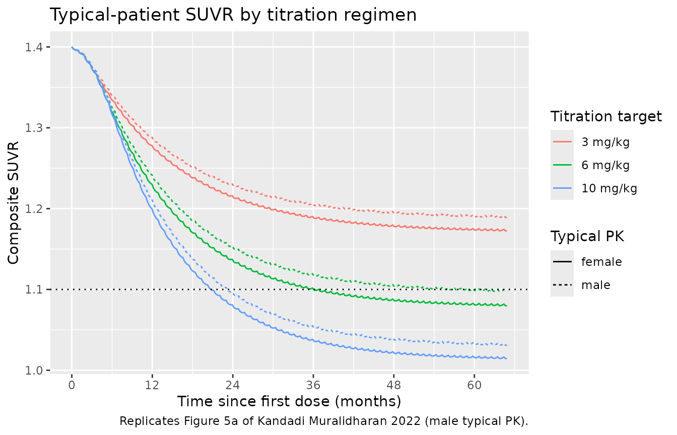
The maintainers digitised the three Figure 5a curves from the article PDF (vector-rendered page, pixel colour extraction calibrated on the gridlines). The table compares them with the typical simulations for each sex:
fig5a <- tibble::tribble(
  ~regimen, ~month, ~fig5a,
  "3 mg/kg", 12, 1.286, "3 mg/kg", 24, 1.230, "3 mg/kg", 36, 1.208,
  "3 mg/kg", 48, 1.199, "3 mg/kg", 60, 1.196,
  "6 mg/kg", 12, 1.240, "6 mg/kg", 24, 1.154, "6 mg/kg", 36, 1.123,
  "6 mg/kg", 48, 1.112, "6 mg/kg", 60, 1.108,
  "10 mg/kg", 12, 1.211, "10 mg/kg", 24, 1.098, "10 mg/kg", 36, 1.059,
  "10 mg/kg", 48, 1.046, "10 mg/kg", 60, 1.041
)
at_month <- function(reg, sx, m) {
  d <- sim_typ[sim_typ$regimen == reg & sim_typ$sex == sx, ]
  approx(d$month, d$suvr, xout = m)$y
}
cmp5a <- fig5a |>
  dplyr::mutate(
    male = mapply(at_month, regimen, "male", month),
    female = mapply(at_month, regimen, "female", month)
  )
cmp5a |>
  dplyr::rename(
    "Regimen" = regimen, "Month" = month, "Figure 5a (digitised)" = fig5a,
    "Simulated, male PK" = male, "Simulated, female PK" = female
  ) |>
knitr::kable(digits = 3, caption = "Typical SUVR: Figure 5a vs. simulation.")| Regimen | Month | Figure 5a (digitised) | Simulated, male PK | Simulated, female PK |
|---|---|---|---|---|
| 3 mg/kg | 12 | 1.286 | 1.288 | 1.277 |
| 3 mg/kg | 24 | 1.230 | 1.230 | 1.215 |
| 3 mg/kg | 36 | 1.208 | 1.205 | 1.189 |
| 3 mg/kg | 48 | 1.199 | 1.195 | 1.178 |
| 3 mg/kg | 60 | 1.196 | 1.190 | 1.174 |
| 6 mg/kg | 12 | 1.240 | 1.241 | 1.229 |
| 6 mg/kg | 24 | 1.154 | 1.153 | 1.136 |
| 6 mg/kg | 36 | 1.123 | 1.118 | 1.100 |
| 6 mg/kg | 48 | 1.112 | 1.104 | 1.087 |
| 6 mg/kg | 60 | 1.108 | 1.099 | 1.081 |
| 10 mg/kg | 12 | 1.211 | 1.210 | 1.199 |
| 10 mg/kg | 24 | 1.098 | 1.096 | 1.080 |
| 10 mg/kg | 36 | 1.059 | 1.054 | 1.037 |
| 10 mg/kg | 48 | 1.046 | 1.038 | 1.022 |
| 10 mg/kg | 60 | 1.041 | 1.032 | 1.016 |
# A deterministic typical-value solve compared against a digitised curve:
# the tolerance covers digitisation error (~0.005 SUVR), not cohort noise.
stopifnot(max(abs(cmp5a$male - cmp5a$fig5a)) < 0.02)
With the male typical PK, the simulation is within 0.009 SUVR units of every digitised point. With the female PK reference, the simulated reduction is 8% larger on average: a female patient has about 12% lower CL (1/1.134), so a higher serum exposure for the same mg/kg dose.
t110 <- sim_typ |>
  dplyr::group_by(regimen, sex) |>
  dplyr::summarise(
    years_to_1.10 = if (any(suvr <= 1.10)) min(month[suvr <= 1.10]) / 12 else NA_real_,
    .groups = "drop"
  )
knitr::kable(t110, digits = 2, caption = "Time for the typical patient to reach SUVR 1.10.")| regimen | sex | years_to_1.10 |
|---|---|---|
| 3 mg/kg | female | NA |
| 3 mg/kg | male | NA |
| 6 mg/kg | female | 3.01 |
| 6 mg/kg | male | 4.64 |
| 10 mg/kg | female | 1.74 |
| 10 mg/kg | male | 1.94 |
The Discussion says the 10 mg/kg regimen takes about 2.25 years to reach SUVR 1.10, more than 4 years for 6 mg/kg, and that 3 mg/kg never gets there. In the digitised Figure 5a, the 10 mg/kg curve crosses 1.10 at about 23.6 months (1.97 years), and the 6 mg/kg curve levels off just above 1.10 (1.107 at 64 months). With male typical PK, the simulated 10 mg/kg patient reaches 1.10 at 1.94 years, in line with the figure. The 6 mg/kg patient reaches it only at 4.6 years, because its plateau sits within 0.01 of the threshold.
Dose interruption (Figure 5b)
Figure 5b models an ARIA event at month 5 in a patient titrated to 10 mg/kg: a 12-week suspension (three missed doses), after which dosing resumes at the dose level used before the suspension and titration continues.
seq_full <- titration("10 mg/kg", n_doses)
# Doses 1-5 given (1, 1, 3, 3, 6 mg/kg at months 0-4); the doses at weeks
# 20, 24 and 28 are missed; dosing resumes at week 32 at 6 mg/kg and the
# titration then continues (6, then 10 mg/kg).
seq_aria <- c(seq_full[1:5], seq_full[6:(n_doses - 3)])
times_aria <- c((0:4) * tau, (8:(n_doses - 1)) * tau)
ev_5b <- dplyr::bind_rows(
  make_subject(1, seq_full, (seq_len(n_doses) - 1) * tau, obs_grid, SEXF = 0),
  make_subject(2, seq_aria, times_aria, obs_grid, SEXF = 0)
)
sim_5b <- rxode2::rxSolve(mod_typical, ev_5b, returnType = "data.frame") |>
  dplyr::mutate(
    month = time / month_h,
    scenario = ifelse(id == 1, "1(2)-3(2)-6(2)-10 mg/kg Q4W", "ARIA-E (12-week interruption at month 5)")
  )
#> ℹ omega/sigma items treated as zero: 'etalvp', 'etalvc', 'etalcl', 'etalec50', 'etalrbase', 'etalemax', 'etalkout', 'etaruv'
#> Warning: multi-subject simulation without without 'omega'
ggplot(sim_5b, aes(month, suvr, linetype = scenario)) +
  geom_line(colour = "darkgreen") +
  geom_hline(yintercept = 1.10, linetype = "dotted") +
  scale_x_continuous(breaks = seq(0, 60, 12)) +
  labs(
    x = "Time since first dose (months)", y = "Composite SUVR", linetype = NULL,
    title = "Effect of an ARIA dose interruption on SUVR",
    caption = "Replicates Figure 5b of Kandadi Muralidharan 2022 (male typical PK)."
  ) +
  theme(legend.position = "bottom")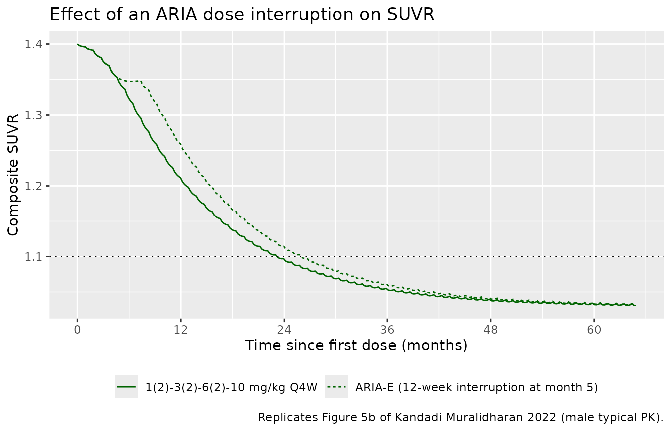
gap <- sim_5b |>
  dplyr::select(time, id, suvr) |>
  tidyr::pivot_wider(names_from = id, values_from = suvr, names_prefix = "id")
gap18 <- approx(gap$time, gap$id2 - gap$id1, xout = 18 * month_h)$y
gap60 <- approx(gap$time, gap$id2 - gap$id1, xout = 60 * month_h)$y
# Deterministic comparison of two typical-value solves.
stopifnot(gap18 > 0.02, abs(gap60) < 0.005)
At month 18 (the week-78 primary end point), the interrupted profile is 0.029 SUVR units above the uninterrupted one; Figure 5b shows a gap of about 0.03. By month 60 the difference is 0.0008, as in the paper, which notes that the influence of the interruption “diminished with time beyond week 78”.
Covariate effect on SUVR change at 30 months (Figure 3b)
Figure 3b gives the typical change from baseline in SUVR (DeltaSUVR) at 30 months after titration to 10 mg/kg: 0.335 for the reference patient, and 0.23 and 0.42 for 57- and 82-year-old patients (the Discussion; 5th and 95th age percentiles). Age acts on both the baseline SUVR (exponent 0.101) and Emax (exponent 1.94, Model S2), so this figure checks the age-on-Emax term, which Table 2 does not print.
fig3b <- tibble::tibble(
  scenario = c("Reference (71 years)", "Age 57 years", "Age 82 years"),
  AGE = c(71, 57, 82),
  published = c(0.335, 0.23, 0.42)
)
ev_3b <- dplyr::bind_rows(lapply(seq_len(nrow(fig3b)), function(i) {
  make_subject(
    id = i, dose_mgkg = titration("10 mg/kg", 33),
    dose_times = (0:32) * tau, obs_times = c(0, 30 * month_h),
    AGE = fig3b$AGE[i], SEXF = 0
  )
}))
sim_3b <- rxode2::rxSolve(mod_typical, ev_3b, returnType = "data.frame")
#> ℹ omega/sigma items treated as zero: 'etalvp', 'etalvc', 'etalcl', 'etalec50', 'etalrbase', 'etalemax', 'etalkout', 'etaruv'
#> Warning: multi-subject simulation without without 'omega'
fig3b$simulated <- sapply(seq_len(nrow(fig3b)), function(i) {
  s <- sim_3b[sim_3b$id == i, ]
  s$suvr[s$time == 0] - s$suvr[s$time == 30 * month_h]
})
fig3b$pct_diff <- 100 * (fig3b$simulated - fig3b$published) / fig3b$published
fig3b |>
  dplyr::select(-AGE) |>
  dplyr::rename(
    "Scenario" = scenario, "Published DeltaSUVR" = published,
    "Simulated DeltaSUVR" = simulated, "Difference (%)" = pct_diff
  ) |>
knitr::kable(digits = 3, caption = "DeltaSUVR at 30 months: Figure 3b vs. typical simulation (male PK).")| Scenario | Published DeltaSUVR | Simulated DeltaSUVR | Difference (%) |
|---|---|---|---|
| Reference (71 years) | 0.335 | 0.331 | -1.079 |
| Age 57 years | 0.230 | 0.227 | -1.396 |
| Age 82 years | 0.420 | 0.418 | -0.450 |
Stochastic cohort
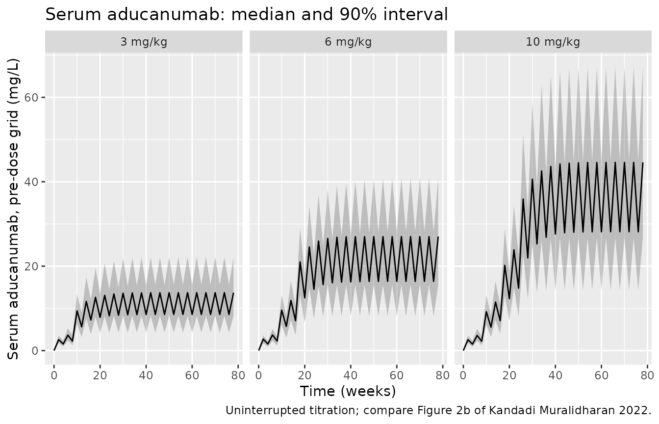
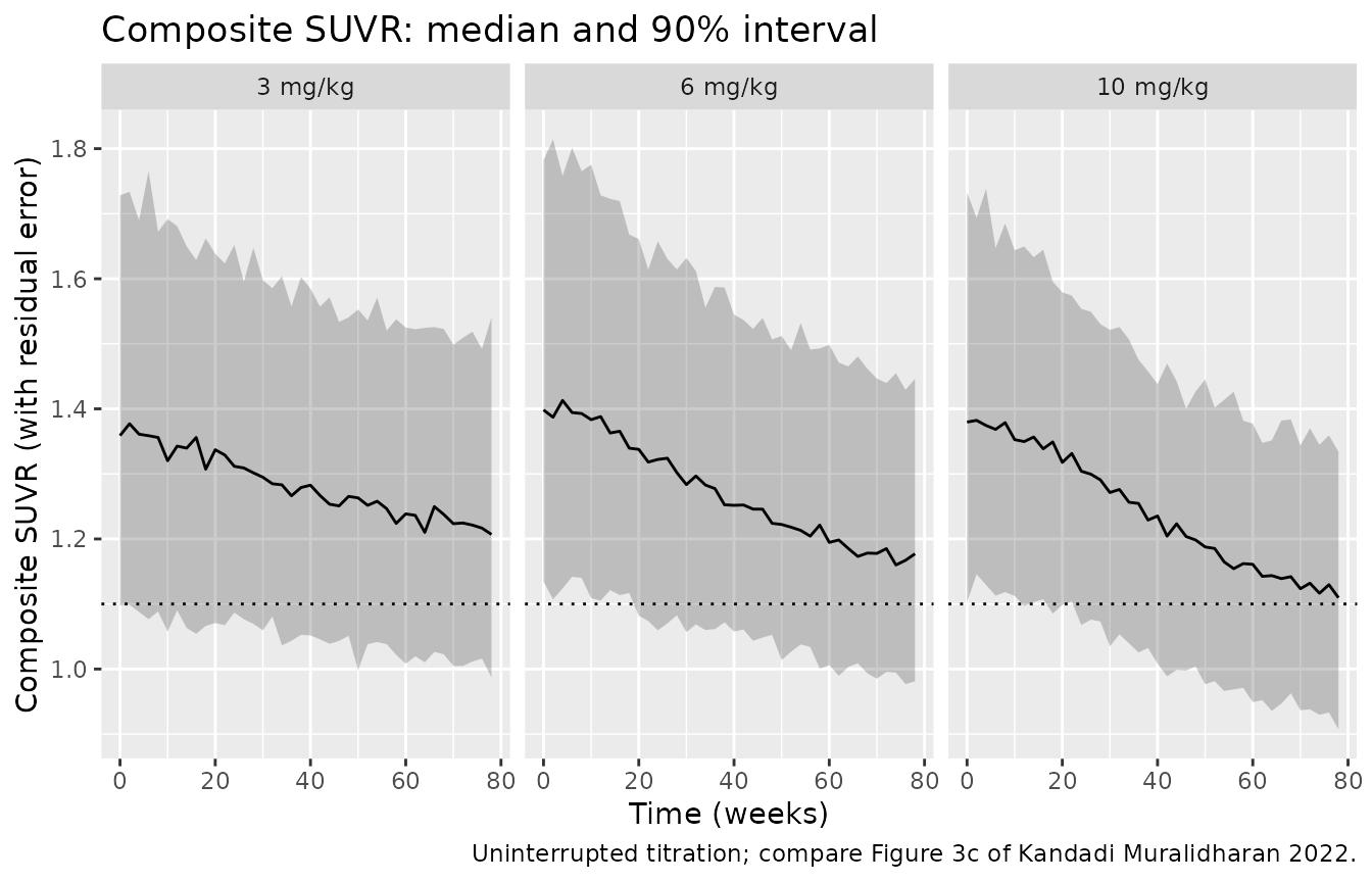
The pcVPCs in Figures 2b and 3c are conditional on the dosing histories actually observed in the trials, including the ARIA interruptions and protocol-amendment dose changes, so they cannot be reproduced from the publication. The simulation below instead gives 150 virtual patients per arm the three uninterrupted titration regimens over the 78-week placebo-controlled period (20 infusions), and shows the variability the model implies.
rxode2::rxSetSeed(20220107)
set.seed(20220107)
n_per_arm <- 150
n_pc_doses <- 20
obs_pc <- sort(unique(c(
  seq(0, 78 * 7 * 24, by = 14 * 24),
  52 * 7 * 24 + c(0, 1, 2, 4, 8, 12, 24, 48, 96, 168, 336, 504, 671)
)))

make_cohort <- function(n, regimen, id_offset) {
  cov <- tibble::tibble(
    id = id_offset + seq_len(n),
    WT = pmin(pmax(rnorm(n, 71.6, 13), 40), 140),
    AGE = pmin(pmax(rnorm(n, 70.3, 7.5), 50), 91),
    SEXF = rbinom(n, 1, 0.52),
    RACE_ASIAN = rbinom(n, 1, 0.10),
    SCORE_MMSE = round(pmin(pmax(rnorm(n, 26, 1.8), 20), 30)),
    apoe = sample(c("non", "het", "hom"), n, replace = TRUE, prob = c(0.31, 0.51, 0.18))
  )
  dplyr::bind_rows(lapply(seq_len(n), function(i) {
    make_subject(
      id = cov$id[i], dose_mgkg = titration(regimen, n_pc_doses),
      dose_times = (seq_len(n_pc_doses) - 1) * tau, obs_times = obs_pc,
      WT = cov$WT[i], AGE = cov$AGE[i], SEXF = cov$SEXF[i],
      RACE_ASIAN = cov$RACE_ASIAN[i], SCORE_MMSE = cov$SCORE_MMSE[i],
      APOE4_HET = as.integer(cov$apoe[i] == "het"),
      APOE4_HOM = as.integer(cov$apoe[i] == "hom")
    )
  })) |>
    dplyr::mutate(treatment = regimen)
}
events <- dplyr::bind_rows(
  make_cohort(n_per_arm, "3 mg/kg", 0L),
  make_cohort(n_per_arm, "6 mg/kg", n_per_arm),
  make_cohort(n_per_arm, "10 mg/kg", 2L * n_per_arm)
)
stopifnot(!anyDuplicated(unique(events[, c("id", "time", "evid")])))

sim <- rxode2::rxSolve(mod, events, keep = "treatment", returnType = "data.frame") |>
  dplyr::mutate(treatment = factor(treatment, levels = regimens), week = time / (7 * 24))
sim |>
  dplyr::filter(time %in% seq(0, 78 * 7 * 24, by = 14 * 24)) |>
  dplyr::group_by(treatment, week) |>
  dplyr::summarise(
    Q05 = quantile(Cc, 0.05), Q50 = median(Cc), Q95 = quantile(Cc, 0.95),
    .groups = "drop"
  ) |>
  ggplot(aes(week, Q50)) +
  geom_ribbon(aes(ymin = Q05, ymax = Q95), alpha = 0.25) +
  geom_line() +
  facet_wrap(~treatment) +
  labs(
    x = "Time (weeks)", y = "Serum aducanumab, pre-dose grid (mg/L)",
    title = "Serum aducanumab: median and 90% interval",
    caption = "Uninterrupted titration; compare Figure 2b of Kandadi Muralidharan 2022."
  )
sim |>
  dplyr::filter(time %in% seq(0, 78 * 7 * 24, by = 14 * 24)) |>
  dplyr::group_by(treatment, week) |>
  dplyr::summarise(
    Q05 = quantile(sim, 0.05), Q50 = median(sim), Q95 = quantile(sim, 0.95),
    .groups = "drop"
  ) |>
  ggplot(aes(week, Q50)) +
  geom_ribbon(aes(ymin = Q05, ymax = Q95), alpha = 0.25) +
  geom_line() +
  geom_hline(yintercept = 1.10, linetype = "dotted") +
  facet_wrap(~treatment) +
  labs(
    x = "Time (weeks)", y = "Composite SUVR (with residual error)",
    title = "Composite SUVR: median and 90% interval",
    caption = "Uninterrupted titration; compare Figure 3c of Kandadi Muralidharan 2022."
  )
PKNCA validation
Steady-state dosing interval
The paper reports no NCA of its own. PKNCA is run over the week 52-56 dosing interval of the stochastic cohort. By then every arm has been on its maintenance dose for at least 34 weeks, about 10 half-lives. Times are re-anchored to the start of the interval.
t0 <- 52 * 7 * 24
sim_nca <- sim |>
  dplyr::filter(!is.na(Cc), time >= t0, time <= t0 + tau) |>
  dplyr::transmute(id, treatment, time = time - t0, Cc)
dose_nca <- events |>
  dplyr::filter(evid == 1, time == t0) |>
  dplyr::transmute(id, treatment, time = 0, amt)
conc_obj <- PKNCA::PKNCAconc(sim_nca, Cc ~ time | treatment + id)
dose_obj <- PKNCA::PKNCAdose(dose_nca, amt ~ time | treatment + id)
intervals <- data.frame(
  start = 0, end = tau, cmax = TRUE, tmax = TRUE, cmin = TRUE,
  auclast = TRUE, cav = TRUE
)
nca_ss <- PKNCA::pk.nca(PKNCA::PKNCAdata(conc_obj, dose_obj, intervals = intervals))
knitr::kable(
  summary(nca_ss),
  caption = "Simulated steady-state NCA (week 52-56 interval) by titration target."
)| start | end | treatment | N | auclast | cmax | cmin | tmax | cav |
|---|---|---|---|---|---|---|---|---|
| 0 | 672 | 10 mg/kg | 150 | 42100 [23.7] | 216 [18.3] | 26.8 [38.6] | 1.00 [1.00, 1.00] | 62.6 [23.7] |
| 0 | 672 | 3 mg/kg | 150 | 12800 [24.5] | 63.3 [19.5] | 8.40 [40.6] | 1.00 [1.00, 1.00] | 19.1 [24.5] |
| 0 | 672 | 6 mg/kg | 150 | 25000 [24.5] | 129 [17.4] | 15.8 [40.0] | 1.00 [1.00, 1.00] | 37.2 [24.5] |
Because PK is linear, each subject’s average steady-state
concentration equals dose / (CL x tau). Below, the simulated
cav at 10 mg/kg is compared subject by subject with that
closed form, using each subject’s own CL:
cav_10 <- as.data.frame(nca_ss) |>
  dplyr::filter(PPTESTCD == "cav", treatment == "10 mg/kg")
ind <- sim |>
  dplyr::filter(treatment == "10 mg/kg", time == t0) |>
  dplyr::select(id, cl) |>
  dplyr::left_join(events |> dplyr::filter(evid == 1, time == t0) |> dplyr::select(id, amt), by = "id")
cav_closed <- ind$amt / (ind$cl * tau)
cav_cmp <- dplyr::left_join(cav_10 |> dplyr::select(id, PPORRES), data.frame(id = ind$id, closed = cav_closed), by = "id")
# Same drawn parameters on both sides: the only difference is trapezoidal
# error on a smooth steady-state profile plus residual non-stationarity.
stopifnot(abs(median(cav_cmp$PPORRES / cav_cmp$closed - 1)) < 0.03)
Half-life
The paper reports an effective half-life of about 24.8 days for the reference patient (female, White, 70.9 kg, age 71, MMSE 26). Individual estimates ranged from 14.8 to 37.9 days (5th and 95th percentiles; Discussion). The effective half-life is calculated from the accumulation ratio R of the steady-state and first-dose troughs for 10 mg/kg Q4W: HLeff = 0.6932 tau / ln(R / (R - 1)) (Appendix S1). The same calculation is applied to the typical reference patient and to 200 virtual patients. PKNCA also estimates the terminal half-life after a single 10 mg/kg dose.
n_hl <- 13 # 12 doses bring the trough to steady state; trough taken before dose 13
ev_hl_typ <- make_subject(1, rep(10, n_hl), (0:(n_hl - 1)) * tau, c(tau, n_hl * tau) - 0.01)
s_hl <- rxode2::rxSolve(mod_typical, ev_hl_typ, returnType = "data.frame")
#> ℹ omega/sigma items treated as zero: 'etalvp', 'etalvc', 'etalcl', 'etalec50', 'etalrbase', 'etalemax', 'etalkout', 'etaruv'
hl_eff <- function(c1, css) {
  R <- css / c1
  0.6932 * tau / log(R / (R - 1)) / 24
}
hl_typ <- hl_eff(s_hl$Cc[1], s_hl$Cc[2])

rxode2::rxSetSeed(20220108)
set.seed(20220108)
n_hlc <- 200
cov_hl <- tibble::tibble(
  WT = pmin(pmax(rnorm(n_hlc, 71.6, 13), 40), 140),
  AGE = pmin(pmax(rnorm(n_hlc, 70.3, 7.5), 50), 91),
  SEXF = rbinom(n_hlc, 1, 0.52),
  RACE_ASIAN = rbinom(n_hlc, 1, 0.10),
  SCORE_MMSE = round(pmin(pmax(rnorm(n_hlc, 26, 1.8), 20), 30))
)
ev_hl <- dplyr::bind_rows(lapply(seq_len(n_hlc), function(i) {
  make_subject(
    i, rep(10, n_hl), (0:(n_hl - 1)) * tau, c(tau, n_hl * tau) - 0.01,
    WT = cov_hl$WT[i], AGE = cov_hl$AGE[i], SEXF = cov_hl$SEXF[i],
    RACE_ASIAN = cov_hl$RACE_ASIAN[i], SCORE_MMSE = cov_hl$SCORE_MMSE[i]
  )
}))
s_hlc <- rxode2::rxSolve(mod, ev_hl, returnType = "data.frame") |>
  dplyr::arrange(id, time) |>
  dplyr::group_by(id) |>
  dplyr::summarise(hl = hl_eff(Cc[1], Cc[2]), .groups = "drop")
hl_q <- quantile(s_hlc$hl, c(0.05, 0.5, 0.95))
data.frame(
  quantity = c("Reference patient", "Cohort 5th percentile", "Cohort median", "Cohort 95th percentile"),
  published_days = c(24.8, 14.8, NA, 37.9),
  simulated_days = c(hl_typ, unname(hl_q))
) |>
  dplyr::rename("Effective half-life" = quantity, "Published (days)" = published_days, "Simulated (days)" = simulated_days) |>
knitr::kable(digits = 1, caption = "Effective half-life from the trough accumulation ratio (10 mg/kg Q4W).")| Effective half-life | Published (days) | Simulated (days) |
|---|---|---|
| Reference patient | 24.8 | 24.0 |
| Cohort 5th percentile | 14.8 | 16.9 |
| Cohort median | NA | 23.6 |
| Cohort 95th percentile | 37.9 | 36.0 |
# Typical-value solve: deterministic.
stopifnot(abs(hl_typ / 24.8 - 1) < 0.05)
# Cohort centre only (robust to which subjects land in the tails).
stopifnot(abs(hl_q[[2]] / 24.8 - 1) < 0.15)
ev_sd <- make_subject(1, 10, 0, c(0, 0.5, 1, 2, 4, 8, 24, 48, 72, 168, 336, 504, seq(672, 24 * 7 * 24, by = 336))) |>
  dplyr::mutate(treatment = "10 mg/kg single dose")
s_sd <- rxode2::rxSolve(mod_typical, ev_sd, returnType = "data.frame")
#> ℹ omega/sigma items treated as zero: 'etalvp', 'etalvc', 'etalcl', 'etalec50', 'etalrbase', 'etalemax', 'etalkout', 'etaruv'
if (is.null(s_sd$id)) s_sd$id <- 1L
s_sd$treatment <- "10 mg/kg single dose"
conc_sd <- PKNCA::PKNCAconc(dplyr::filter(s_sd, !is.na(Cc)), Cc ~ time | treatment + id)
dose_sd <- PKNCA::PKNCAdose(dplyr::filter(ev_sd, evid == 1), amt ~ time | treatment + id)
nca_sd <- PKNCA::pk.nca(PKNCA::PKNCAdata(
  conc_sd, dose_sd,
  intervals = data.frame(start = 0, end = Inf, cmax = TRUE, tmax = TRUE, aucinf.obs = TRUE, half.life = TRUE)
))
published_hl <- tibble::tibble(treatment = "10 mg/kg single dose", half.life = 24.8 * 24)
cmp_sd <- nlmixr2lib::ncaComparisonTable(
  simulated = nca_sd,
  reference = published_hl,
  by = "treatment",
  params = "half.life",
  units = c(half.life = "h"),
  tolerance_pct = 20
)
knitr::kable(
  cmp_sd,
  caption = "Typical terminal half-life after a single 10 mg/kg dose vs. the published 24.8-day effective half-life. * differs by >20%."
)| NCA parameter | treatment | Reference | Simulated | % diff |
|---|---|---|---|---|
| t½ (h) | 10 mg/kg single dose | 595 | 576 | -3.2% |
For the reference patient, the effective half-life from trough accumulation is 24.0 days. The terminal half-life after a single dose (the beta phase of the two-compartment model) is about the same. Both are within 5% of the published 24.8 days. The cohort 5th-95th percentile range, 16.9-36.0 days, is close to the published 14.8-37.9 days, even though it comes from a virtual rather than the observed covariate distribution.
Assumptions and deviations
- Sex of the typical patient in Figures 3b and 5. The PD reference patient in the figure captions (ApoE4 heterozygote, age 71 years, MMSE 26, 70.9 kg) has no stated sex, and sex affects only the PK layer. Male typical PK reproduces Figure 5a to within 0.01 SUVR and Figure 3b to within 2%. The female PK reference of Table 1 gives an SUVR reduction about 8% larger. The figures were therefore replicated with male typical PK; no parameter was changed.
- Time to SUVR 1.10. The Discussion’s “approximately 2.25 years” at 10 mg/kg does not match the paper’s own Figure 5a, in which the curve crosses 1.10 at about 1.97 years. The simulation follows the figure.
- Age effect on Emax. Table 2 prints no row for the age-on-Emax covariate that the Results name. Its exponent (1.94016) comes from THETA(11) of the final Model S2 control stream, whose other THETAs equal the Table 2 estimates. The Figure 3b age extremes, which depend on it, are reproduced.
-
PK values from Table 1, not Model S1
$THETA. The Model S1$THETAblock holds initial estimates that differ slightly from the Table 1 final estimates (for example the MMSE exponent on V2 is 0.236 there and 0.182 in Table 1). Table 1 is used throughout. -
Omega scales. Table 1 PK %CVs follow footnote b,
%CV = 100 sqrt(exp(omega^2) - 1). The Model S1 omegas reproduce the
printed %CV and correlations under that formula, so omega^2 = log(1 +
CV^2) was used. For Table 2, the printed %CVs equal 100 sqrt(omega^2) of
the final Model S2
$OMEGAestimates, despite the same footnote; the Model S2 values are used directly. - Reference weights. The Results text says the reference patient weighs “71.9 kg”. The control stream and the Figure 2 and Figure 3 captions all use 70.9 kg, which is used here. Kout is referenced to 72 kg in Model S2.
-
Residual variability. Model S1 scales the whole
combined residual SD
sqrt((0.148 IPRED)^2 + 0.202^2)byexp(eta)per subject. This is encoded withetaruvon both components andcombined2(). The convention checker warns thatetaruvhas no matching fixed effect; that is expected for IIV on residual error (the same structure is used byXie_2019_tofacitinib). The SUVR residual is proportional only, because the additive term was fixed to 0 when placebo data were added (Table S5, run 75). -
ApoE4 coding. The model’s reference genotype is the
heterozygote, as in Model S2. Non-carriers have
APOE4_HET = APOE4_HOM = 0and receive the non-carrier multiplier. - Infusion duration. The paper does not state it. The example data rows in Model S1 show infusion times of 1.0-2.2 h, so 1 h was used; this has no visible effect on a 4-weekly profile.
- Virtual cohort. Weight, age and MMSE were drawn from truncated normal distributions matching the Table S2 means and ranges, and sex, ApoE4 genotype and Asian race from binomial and multinomial draws (Asian 10%, assumed: the paper reports only 79% Caucasian). The phase III titration sequences follow the Figure 5a legend; the uninterrupted regimens do not represent the dosing actually delivered in ENGAGE and EMERGE.
- No erratum or correction notice for this article was found in Europe PMC (checked 2026-09-30).