Tapentadol from birth to <18 years (Khalil 2020)
Source:vignettes/articles/Khalil_2020_tapentadol.Rmd
Khalil_2020_tapentadol.RmdModel and source
#> ℹ parameter labels from comments will be replaced by 'label()'
#> ℹ parameter labels from comments will be replaced by 'label()'
Citation: Khalil F, Choi SL, Watson E, Tzschentke TM, Lefeber C, Eerdekens M, Freijer J. Population Pharmacokinetics of Tapentadol in Children from Birth to <18 Years Old. J Pain Res. 2020;13:3107-3123. doi:10.2147/JPR.S269549
Khalil_2020_tapentadol_allometryFixed: One-compartment population PK model for tapentadol oral solution and 1-hour intravenous infusion in 148 children from birth (including preterm neonates) to <18 years with acute pain (Khalil 2020), the variant with the allometric exponents FIXED to the theoretical 0.75 (CL) and 1 (V). First-order absorption from a depot preceded by an absorption lag time, first-order elimination. CL and V are systemic (IV data identify F). CL carries a hyperbolic (Hill fixed to 1) postmenstrual-age maturation function; oral bioavailability decays exponentially with postnatal age from twice the adult value at birth to the adult value. Log-normal IIV on CL, V (correlated) and Ka; combined proportional plus additive residual error. The companion Khalil_2020_tapentadol_allometryEstimated model estimates the two exponents instead.Khalil_2020_tapentadol_allometryEstimated: One-compartment population PK model for tapentadol oral solution and 1-hour intravenous infusion in 148 children from birth (including preterm neonates) to <18 years with acute pain (Khalil 2020), the variant with the allometric exponents ESTIMATED (0.603 on CL, 0.820 on V; theory 0.75 and 1). First-order absorption from a depot preceded by an absorption lag time, first-order elimination. CL and V are systemic (IV data identify F). CL carries a hyperbolic (Hill fixed to 1) postmenstrual-age maturation function; oral bioavailability decays exponentially with postnatal age from twice the adult value at birth to the adult value. Log-normal IIV on CL, V (correlated) and Ka; combined proportional plus additive residual error. The companion Khalil_2020_tapentadol_allometryFixed model fixes the two exponents to 0.75 and 1; the estimated-exponent model has the lower OFV (delta OFV -13.12 for 2 extra parameters).Article: https://doi.org/10.2147/JPR.S269549 (open access; J Pain Res. 2020;13:3107-3123, PMC7700087)
Khalil 2020 pools four single-dose phase 2 trials of tapentadol in
children with acute pain: two oral-solution trials in children 2 to
<18 years (the data behind Watson_2019_tapentadol), an
oral-solution trial from birth to <2 years, and a 1-hour
intravenous-infusion trial from preterm birth to <2 years. The IV arm
identifies oral bioavailability, so clearance and volume are systemic.
The authors fit the same one-compartment structure twice – once with the
allometric exponents fixed to the theoretical 0.75 (CL) and 1 (V) and
once with both estimated – and report both as final models (Table 3).
Both are packaged:
-
Khalil_2020_tapentadol_allometryFixed– exponents fixed at 0.75 / 1. -
Khalil_2020_tapentadol_allometryEstimated– exponents estimated (0.603 / 0.820); lower objective function (delta OFV -13.12 for two extra parameters).
In both, clearance carries a hyperbolic postmenstrual-age maturation function and oral bioavailability decays exponentially with postnatal age from twice its adult value at birth:
- CL = CL_TV * PMA / (PMA + PMA50) * (WT / 70)^n (Methods equation 1)
- V = V_TV * (WT / 70)^n (Methods equation 2)
- F = F_adult * (1 + exp(-k * PNA)) (Methods equation 3)
PMA and PNA are in weeks in the paper. The packaged models take
PAGE in weeks (as the paper does) and the canonical
PNA in months, converted inside model() with
30.4375 / 7 weeks per month.
Population
| Field | Value |
|---|---|
| species | human |
| n_subjects | 148 |
| n_studies | 4 |
| n_observations | 569 quantifiable tapentadol serum concentrations (Khalil 2020 Methods, ‘Population Pharmacokinetic Modeling Data Set’) |
| age_range | Birth (including preterm neonates, gestational age >=24 weeks) to <18 years; group medians 15 y, 9 y, 3 y, 14 months, 3 months, 12 days (term neonates) and 12 days (preterm) (Table 1) |
| weight_range | 1.6-80 kg; group medians 59.7, 29.5, 16.4, 10, 5.9, 3.6 and 2.45 kg (Table 1) |
| sex_female_pct | 45.9 |
| disease_state | Acute pain (mostly postsurgical or procedural) severe enough to require an opioid |
| dose_range | Single dose. Oral solution 1.0 mg/kg (>=2 years), 0.75 mg/kg (6 months to <2 years), 0.6 mg/kg (1 to <6 months), 0.5 mg/kg (birth to <1 month); IV 1-hour infusion 0.4 mg/kg (<2 years) or 0.3-0.4 mg/kg (preterm, by gestational and postnatal age) (Table 1) |
| regions | Multinational (trial sites listed in the paper’s supplement) |
| notes | Pooled from four single-dose open-label phase 2 PK trials: NCT01729728 (n=56) and NCT01134536 (n=36), oral solution, 2 to <18 years; NCT02221674 (n=18), oral solution, birth to <2 years (term); EudraCT 2014-002259-24 (n=38), IV, preterm to <2 years (Table 2). Preterm neonates were dosed IV only. Female percentage (45.9%) is the N-weighted sum of Table 1’s per-group percentages (68/148; Table 2 gives the same 68). 38 oral samples from 17 patients who vomited within 3 h or did not take the full dose, and one contaminated IV sample, were excluded. NONMEM 7.2. |
148 children contributed 569 quantifiable serum concentrations; about 75% of samples came from orally dosed children aged 2 years or older, and 113 concentrations from 38 children came from the IV trial. Children 2 years and older received 1.0 mg/kg oral solution; younger children received 0.75, 0.6 or 0.5 mg/kg orally (6 months to <2 years, 1 to <6 months, birth to <1 month) or 0.4 mg/kg IV over 1 hour; preterm neonates (gestational age 24 to <37 weeks) received 0.3 or 0.4 mg/kg IV only. The sex balance was 68 of 148 female (45.9%).
Source trace
Every ini() entry in both model files carries an in-file
comment naming its source. They are collected here.
| Equation / parameter | Fixed exponents | Estimated exponents | Source location |
|---|---|---|---|
lcl (CL at 70 kg, mature) |
94.6 L/h | 64.7 L/h | Table 3, row CL (L/h)
|
lvc (V at 70 kg) |
414 L | 270 L | Table 3, row V (L)
|
lka (Ka) |
2.19 1/h | 2.16 1/h | Table 3, row Ka (h-1)
|
lfdepot (F_adult) |
0.349 | 0.265 | Table 3, row F
|
ltlag (TLAG) |
0.266 h | 0.266 h | Table 3, row TLAG (h)
|
ltm50_cl (PMA50) |
34.8 weeks | 36.7 weeks | Table 3, row PMA50 (wks)
|
hill_mat |
1 (fixed) | 1 (fixed) | Table 3, row HILL exponent
|
e_pna_fdepot (k) |
0.122 1/week | 0.0599 1/week | Table 3, row k (wks-1)
|
e_wt_cl |
0.75 (fixed) | 0.603 | Table 3, row Exponent CL-WT
|
e_wt_vc |
1 (fixed) | 0.82 | Table 3, row Exponent V-WT
|
etalcl variance |
0.0961 | 0.0892 | Table 3, row IIV CL (omega2)
|
etalvc variance |
0.13 | 0.115 | Table 3, row IIV V (omega2)
|
cov(etalcl, etalvc) |
0.0867 | 0.0752 | Table 3, row Cov CL-V
|
etalka variance |
2 | 1.96 | Table 3, row IIV Ka (omega2)
|
propSd |
0.327 | 0.326 | Table 3, row Proportional error (sigma)
|
addSd |
0.48 ng/mL | 0.494 ng/mL | Table 3, row Additive error (ng/mL)
|
| CL maturation and allometry | Methods, equation 1 (reference weight 70 kg) | ||
| V allometry | Methods, equation 2 | ||
F maturation F = F_adult (1 + exp(-k PNA))
|
Methods, equation 3 | ||
IIV Pi = PTV exp(eta_i)
|
Methods, equation 4 | ||
Residual Co = Cp (1 + eps_p) + eps_a
|
Methods, equation 5 | ||
| PMA = GA + PNA; GA = 40 weeks at term | Methods, “Simulation of Virtual Pediatric Population” | ||
| 1-hour IV infusion | Methods, “Clinical Trial Design” |
Deterministic structural checks
These compare the packaged parameters against numbers Khalil 2020 prints outside Table 3. No random draws are involved, so tight tolerances are appropriate.
th <- lapply(uis, function(u) {
  x <- setNames(u$iniDf$est, u$iniDf$name)
  x[!is.na(u$iniDf$name) & is.na(u$iniDf$neta1)]
})
typ <- function(m, nm) unname(th[[m]][[nm]])

# Discussion, 'Estimated versus Assumed Allometric Exponents': at full maturation
# and 70 kg, CL/F = 271 and 244 L/h and V/F = 1186 and 1018 L.
adult <- tibble::tibble(
  model = names(stems),
  clf_paper = c(271, 244),
  vf_paper = c(1186, 1018),
  clf_model = c(exp(typ("fixed", "lcl") - typ("fixed", "lfdepot")),
                exp(typ("estimated", "lcl") - typ("estimated", "lfdepot"))),
  vf_model = c(exp(typ("fixed", "lvc") - typ("fixed", "lfdepot")),
               exp(typ("estimated", "lvc") - typ("estimated", "lfdepot")))
)
adult |>
  rename(
    "Model" = model,
    "CL/F paper (L/h)" = clf_paper, "CL/F model (L/h)" = clf_model,
    "V/F paper (L)" = vf_paper, "V/F model (L)" = vf_model
  ) |>
knitr::kable(digits = 1, caption = "Adult (70 kg, fully mature) apparent parameters: Khalil 2020 Discussion vs the packaged Table 3 values.")| Model | CL/F paper (L/h) | V/F paper (L) | CL/F model (L/h) | V/F model (L) |
|---|---|---|---|---|
| fixed | 271 | 1186 | 271.1 | 1186.2 |
| estimated | 244 | 1018 | 244.2 | 1018.9 |
# Discussion, 'Factors Influencing Tapentadol PK Parameters Across Age': with
# PMA50 about 35 weeks, '80% of maturation is expected to be achieved at a PMA
# of about 140 weeks'. For a Hill exponent of 1, PMA(80%) = 4 * PMA50.
pma80 <- 4 * exp(typ("fixed", "ltm50_cl"))

# Figure 4D (fixed exponents): V/F per kg does not depend on weight when the V
# exponent is 1, so it isolates the F maturation equation. Read off the figure:
# about 8.5 L/kg at birth and 17 L/kg in older children -- a factor of 2 that
# pins down the sign of the exponent in equation 3 (a '+k' would make F grow
# without bound).
vfkg <- function(pna_wk) {
  exp(typ("fixed", "lvc")) / 70 /
    (exp(typ("fixed", "lfdepot")) * (1 + exp(-typ("fixed", "e_pna_fdepot") * pna_wk)))
}
vfkg_birth <- vfkg(0)
vfkg_mature <- vfkg(18 * 52)

# Discussion: 'maximum serum concentrations ... after a single oral solution
# dose in pediatrics were typically observed at around 1.3-1.5 h'. Typical
# value at the 12 to <18 year Table 1 median (15 y, 59.7 kg), fully mature.
tmax_typ <- function(m, wt) {
  cl <- exp(typ(m, "lcl")) * (wt / 70)^typ(m, "e_wt_cl")
  v <- exp(typ(m, "lvc")) * (wt / 70)^typ(m, "e_wt_vc")
  ka <- exp(typ(m, "lka"))
  kel <- cl / v
  exp(typ(m, "ltlag")) + log(ka / kel) / (ka - kel)
}
tmax15 <- c(fixed = tmax_typ("fixed", 59.7), estimated = tmax_typ("estimated", 59.7))

cat(sprintf("PMA at 80%% CL maturation: %.1f weeks (paper: about 140)\n", pma80))
#> PMA at 80% CL maturation: 139.2 weeks (paper: about 140)
cat(sprintf("V/F per kg (fixed exponents): %.2f L/kg at birth, %.2f L/kg mature (Figure 4D: ~8.5, ~17)\n",
            vfkg_birth, vfkg_mature))
#> V/F per kg (fixed exponents): 8.47 L/kg at birth, 16.95 L/kg mature (Figure 4D: ~8.5, ~17)
cat(sprintf("Typical Tmax at 59.7 kg: %.2f h (fixed), %.2f h (estimated); paper 1.3-1.5 h\n",
            tmax15[["fixed"]], tmax15[["estimated"]]))
#> Typical Tmax at 59.7 kg: 1.40 h (fixed), 1.40 h (estimated); paper 1.3-1.5 h

stopifnot(
  # The Discussion quotes these to the nearest litre / L/h.
  all(abs(adult$clf_model - adult$clf_paper) < 1),
  all(abs(adult$vf_model - adult$vf_paper) < 1.5),
  abs(pma80 - 140) < 2,
  # Figure reads are to roughly 0.3 L/kg.
  abs(vfkg_birth - 8.5) < 0.5,
  abs(vfkg_mature - 17) < 0.5,
  all(tmax15 > 1.3 & tmax15 < 1.5)
)
Both OMEGA blocks must be positive definite for rxode2’s sampler; that is arithmetic on fixed numbers.
Replicate Figures 6 and 7: steady-state exposure by age group
Figures 6 and 7 show the simulated AUCtau,ss for q4h dosing at each
trial’s dose. For a linear model AUCtau,ss equals the single-dose
AUC(0-inf), which is F * Dose / CL. The typical child of
each group is taken at its Table 1 median age and weight. The figure
medians were digitised by the maintainers from the published boxplots
(reading precision about 10 h*ng/mL).
arms <- tibble::tribble(
  ~arm, ~route, ~pna_mo, ~wt, ~ga, ~dose_mgkg, ~fig6, ~fig7,
  "12 to <18 y PO", "PO", 15 * 12, 59.7, 40, 1.0, 252, 268,
  "6 to <12 y PO", "PO", 9 * 12, 29.5, 40, 1.0, 225, 212,
  "2 to <6 y PO", "PO", 3 * 12, 16.4, 40, 1.0, 215, 188,
  "6 mo to <2 y PO", "PO", 14, 10.0, 40, 0.75, 158, 145,
  "6 mo to <2 y IV", "IV", 14, 10.0, 40, 0.4, 245, 285,
  "1 to <6 mo PO", "PO", 3, 5.9, 40, 0.6, 163, 153,
  "1 to <6 mo IV", "IV", 3, 5.9, 40, 0.4, 258, 277,
  "Birth to <1 mo PO", "PO", 12 / 30.4375, 3.6, 40, 0.5, 205, 160,
  "Birth to <1 mo IV", "IV", 12 / 30.4375, 3.6, 40, 0.4, 275, 265,
  "Preterm IV", "IV", 12 / 30.4375, 2.45, 30.5, 0.3, 218, 220
)

auc_typ <- function(m, d) {
  pna_wk <- d$pna_mo * 30.4375 / 7
  pma <- d$ga + pna_wk
  tm50 <- exp(typ(m, "ltm50_cl"))
  cl <- exp(typ(m, "lcl")) * pma / (pma + tm50) * (d$wt / 70)^typ(m, "e_wt_cl")
  f <- ifelse(d$route == "PO",
              exp(typ(m, "lfdepot")) * (1 + exp(-typ(m, "e_pna_fdepot") * pna_wk)), 1)
  f * d$dose_mgkg * d$wt / cl * 1000 # mg/L*h -> ng*h/mL
}
arms <- arms |>
  mutate(
    auc_fixed = auc_typ("fixed", arms),
    auc_est = auc_typ("estimated", arms),
    pct_fixed = 100 * (auc_fixed - fig6) / fig6,
    pct_est = 100 * (auc_est - fig7) / fig7
  )
arms |>
  select(arm, fig6, auc_fixed, pct_fixed, fig7, auc_est, pct_est) |>
  rename(
    "Age group / route" = arm,
    "Fig 6 median" = fig6, "Fixed-exp typical" = auc_fixed, "Fixed % diff" = pct_fixed,
    "Fig 7 median" = fig7, "Estimated-exp typical" = auc_est, "Estimated % diff" = pct_est
  ) |>
knitr::kable(digits = 1, caption = "Typical-value AUCtau,ss (h*ng/mL) at each Table 1 group median vs the digitised medians of Khalil 2020 Figures 6 (fixed exponents) and 7 (estimated exponents).")| Age group / route | Fig 6 median | Fixed-exp typical | Fixed % diff | Fig 7 median | Estimated-exp typical | Estimated % diff |
|---|---|---|---|---|---|---|
| 12 to <18 y PO | 252 | 258.7 | 2.6 | 268 | 281.2 | 4.9 |
| 6 to <12 y PO | 225 | 222.3 | -1.2 | 212 | 218.1 | 2.9 |
| 2 to <6 y PO | 215 | 211.5 | -1.6 | 188 | 191.3 | 1.7 |
| 6 mo to <2 y PO | 158 | 160.2 | 1.4 | 145 | 139.0 | -4.2 |
| 6 mo to <2 y IV | 245 | 244.7 | -0.1 | 285 | 272.6 | -4.4 |
| 1 to <6 mo PO | 163 | 166.4 | 2.1 | 153 | 158.9 | 3.9 |
| 1 to <6 mo IV | 258 | 264.1 | 2.4 | 277 | 274.2 | -1.0 |
| Birth to <1 mo PO | 205 | 204.3 | -0.3 | 160 | 157.8 | -1.4 |
| Birth to <1 mo IV | 275 | 258.5 | -6.0 | 265 | 250.4 | -5.5 |
| Preterm IV | 218 | 199.7 | -8.4 | 220 | 183.5 | -16.6 |
stopifnot(
  # A mis-transcribed CL, F, k, PMA50 or exponent moves one or more arms by
  # tens of percent. The preterm arm carries an assumed gestational age.
  abs(median(c(arms$pct_fixed, arms$pct_est))) < 5,
  max(abs(c(arms$pct_fixed, arms$pct_est))) < 20
)
Nine of the ten arms reproduce both figures within about 6%. The exception is the preterm IV arm (8% below Figure 6 and 17% below Figure 7). The paper does not state the postnatal ages it simulated for preterm children, and this typical preterm child assumes the median (30.5 weeks) of the paper’s uniform 24 to <37 week gestational-age draw. The estimated-exponent model is the more sensitive of the two here, because its weight exponent on CL is lower (0.603 vs 0.75) and its PMA50 is later (36.7 vs 34.8 weeks).
Virtual cohort
The trial data are not public. The cohort below has 100 children per age-group-and-route arm (10 arms). Postnatal age is drawn uniformly within each group, as in the paper’s simulations. The paper drew weights from the CDC weight-for-age charts; here weight is instead interpolated from the Table 1 group medians of age and weight, with 12% log-normal scatter, redrawn (not clipped) until it falls inside that group’s Table 1 weight range. Preterm children draw gestational age uniformly from 24 to <37 weeks (as in the paper) and weight log-normally about the preterm median of 2.45 kg.
set.seed(20201127)
rxode2::rxSetSeed(20201127)
N_PER_ARM <- 100L

wfa_age <- c(12 / 30.4375, 3, 14, 36, 108, 180) # months (Table 1 medians)
wfa_wt <- c(3.6, 5.9, 10, 16.4, 29.5, 59.7)
groups <- tibble::tribble(
  ~grp, ~pna_lo, ~pna_hi, ~wt_lo, ~wt_hi,
  "12 to <18 y", 144, 216, 41, 80,
  "6 to <12 y", 72, 144, 20.2, 58,
  "2 to <6 y", 24, 72, 12.7, 19.5,
  "6 mo to <2 y", 6, 24, 7.5, 14.2,
  "1 to <6 mo", 1, 6, 4.3, 9,
  "Birth to <1 mo", 0, 1, 2.7, 4.6,
  "Preterm", 0, 1, 1.6, 3.4
)
design <- tibble::tribble(
  ~arm, ~grp, ~route, ~dose_mgkg,
  "12 to <18 y PO", "12 to <18 y", "PO", 1.0,
  "6 to <12 y PO", "6 to <12 y", "PO", 1.0,
  "2 to <6 y PO", "2 to <6 y", "PO", 1.0,
  "6 mo to <2 y PO", "6 mo to <2 y", "PO", 0.75,
  "6 mo to <2 y IV", "6 mo to <2 y", "IV", 0.4,
  "1 to <6 mo PO", "1 to <6 mo", "PO", 0.6,
  "1 to <6 mo IV", "1 to <6 mo", "IV", 0.4,
  "Birth to <1 mo PO", "Birth to <1 mo", "PO", 0.5,
  "Birth to <1 mo IV", "Birth to <1 mo", "IV", 0.4,
  "Preterm IV", "Preterm", "IV", 0.3
) |>
  left_join(groups, by = "grp")

draw_arm <- function(d, n) {
  pna <- stats::runif(n, d$pna_lo, d$pna_hi)
  ga <- if (d$grp == "Preterm") stats::runif(n, 24, 37) else rep(40, n)
  centre <- if (d$grp == "Preterm") rep(2.45, n) else
    stats::approx(wfa_age, wfa_wt, xout = pna, rule = 2)$y
  wt <- centre * exp(stats::rnorm(n, 0, 0.12))
  bad <- wt < d$wt_lo | wt > d$wt_hi
  while (any(bad)) {
    wt[bad] <- centre[bad] * exp(stats::rnorm(sum(bad), 0, 0.12))
    bad <- wt < d$wt_lo | wt > d$wt_hi
  }
  tibble::tibble(arm = d$arm, route = d$route, dose_mgkg = d$dose_mgkg,
                 PNA = pna, GA = ga, WT = wt)
}
cohort <- bind_rows(lapply(seq_len(nrow(design)), function(i) draw_arm(design[i, ], N_PER_ARM))) |>
  mutate(
    id = row_number(),
    PAGE = GA + PNA * 30.4375 / 7,
    dose_mg = dose_mgkg * WT
  )

cohort |>
  group_by(arm) |>
  summarise(n = n(), `median PNA (months)` = median(PNA), `median WT (kg)` = median(WT),
            `min WT` = min(WT), `max WT` = max(WT), .groups = "drop") |>
knitr::kable(digits = 2, caption = "Simulated cohort by arm; compare Khalil 2020 Table 1.")| arm | n | median PNA (months) | median WT (kg) | min WT | max WT |
|---|---|---|---|---|---|
| 1 to <6 mo IV | 100 | 3.69 | 6.11 | 4.30 | 7.82 |
| 1 to <6 mo PO | 100 | 3.37 | 5.86 | 4.30 | 8.04 |
| 12 to <18 y PO | 100 | 180.75 | 55.97 | 42.72 | 79.87 |
| 2 to <6 y PO | 100 | 48.80 | 17.45 | 12.71 | 19.46 |
| 6 mo to <2 y IV | 100 | 15.71 | 10.24 | 7.60 | 14.13 |
| 6 mo to <2 y PO | 100 | 15.38 | 10.51 | 7.50 | 14.16 |
| 6 to <12 y PO | 100 | 100.32 | 29.27 | 20.33 | 50.72 |
| Birth to <1 mo IV | 100 | 0.54 | 3.78 | 2.82 | 4.59 |
| Birth to <1 mo PO | 100 | 0.55 | 3.75 | 2.86 | 4.56 |
| Preterm IV | 100 | 0.60 | 2.45 | 1.88 | 3.21 |
obs_times <- sort(unique(c(seq(0, 3, by = 0.05), seq(3.25, 24, by = 0.25))))
dose_rows <- cohort |>
  transmute(id, time = 0, amt = dose_mg, evid = 1L,
            cmt = ifelse(route == "PO", "depot", "central"),
            rate = ifelse(route == "PO", 0, dose_mg / 1)) # 1-hour IV infusion
obs_rows <- tidyr::expand_grid(id = cohort$id, time = obs_times) |>
  mutate(amt = 0, evid = 0L, cmt = "central", rate = 0)
events <- bind_rows(dose_rows, obs_rows) |>
  left_join(cohort |> select(id, arm, route, WT, PAGE, PNA, dose_mg), by = "id") |>
  arrange(id, time, desc(evid)) |>
  as.data.frame()
Simulation
sims <- lapply(stems, function(s) {
  rxode2::rxSolve(readModelDb(s), events = events,
                  keep = c("arm", "route", "WT", "PAGE", "PNA", "dose_mg")) |>
    as.data.frame()
})
#> ℹ parameter labels from comments will be replaced by 'label()'
#> ℹ parameter labels from comments will be replaced by 'label()'
for (m in names(sims)) {
  s <- sims[[m]]
  stopifnot(nrow(s) > 0L)
  cc_neg <- s$Cc[!is.na(s$Cc) & s$Cc < 0]
  # Round-off of either sign far down the terminal phase is integrator noise;
  # assert it is negligible relative to Cmax before flooring to zero.
  stopifnot(length(cc_neg) == 0L || abs(min(cc_neg)) < 1e-6 * max(s$Cc, na.rm = TRUE))
  sims[[m]]$Cc <- pmax(s$Cc, 0)
}
Replicate Figures 2 and 3
bind_rows(lapply(names(sims), function(m) mutate(sims[[m]], model = m))) |>
  filter(dplyr::between(time, 0.05, 15)) |>
  group_by(model, arm, time) |>
  summarise(Q025 = quantile(sim, 0.025), Q50 = quantile(sim, 0.5),
            Q975 = quantile(sim, 0.975), .groups = "drop") |>
  mutate(arm = factor(arm, levels = design$arm)) |>
  ggplot(aes(time, Q50, colour = model, fill = model)) +
  geom_ribbon(aes(ymin = pmax(Q025, 0.1), ymax = Q975), alpha = 0.15, colour = NA) +
  geom_line(linewidth = 0.7) +
  facet_wrap(~arm, ncol = 3) +
  scale_y_log10() +
  labs(x = "Time (h)", y = "Tapentadol serum concentration (ng/mL)",
       colour = "Exponents", fill = "Exponents") +
  theme_bw() +
  theme(legend.position = "bottom")
#> Warning in transformation$transform(x): NaNs produced
#> Warning in scale_y_log10(): log-10 transformation introduced infinite values.
#> Warning in transformation$transform(x): NaNs produced
#> Warning in scale_y_log10(): log-10 transformation introduced infinite values.
#> Warning: Removed 3 rows containing missing values or values outside the scale range
#> (`geom_line()`).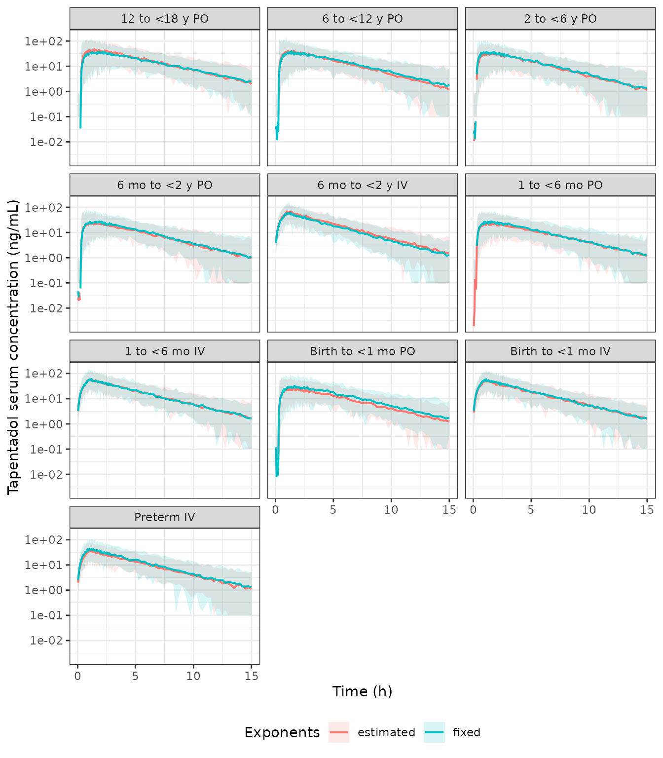
Replicates Figures 2 (fixed exponents) and 3 (estimated exponents) of Khalil 2020: simulated tapentadol serum concentrations after a single dose by age group and route, median (line) and 95% prediction interval including residual error (band), over the 15 h sampling window.
PKNCA validation
Single-dose NCA per arm. For each subject, AUC(0-inf) must equal
F * Dose / CL using the subject’s own simulated
fdepot (1 for IV) and cl; that is the model
checked against its own closed form, so the bound is tight. The per-arm
median AUC(0-inf) is then compared against the digitised Figure 6 and 7
medians, which for a linear model are the same quantity.
nca_one <- function(s) {
  conc <- s |>
    filter(!is.na(Cc)) |>
    select(id, time, Cc, arm)
  conc <- bind_rows(conc, conc |> distinct(id, arm) |> mutate(time = 0, Cc = 0)) |>
    distinct(id, arm, time, .keep_all = TRUE) |>
    arrange(id, time)
  dose <- events |>
    filter(evid == 1L) |>
    select(id, time, amt, arm)
  conc_obj <- PKNCA::PKNCAconc(conc, Cc ~ time | arm + id, concu = "ng/mL", timeu = "h")
  dose_obj <- PKNCA::PKNCAdose(dose, amt ~ time | arm + id, doseu = "mg")
  intervals <- data.frame(start = 0, end = Inf, cmax = TRUE, tmax = TRUE, aucinf.obs = TRUE)
  PKNCA::pk.nca(PKNCA::PKNCAdata(conc_obj, dose_obj, intervals = intervals))
}
ncas <- lapply(sims, nca_one)

for (m in names(sims)) {
  ind <- sims[[m]] |>
    group_by(id) |>
    summarise(route = first(route), dose_mg = first(dose_mg),
              f = ifelse(first(route) == "PO", first(fdepot), 1),
              cl = first(cl), .groups = "drop")
  chk <- as.data.frame(ncas[[m]]$result) |>
    filter(PPTESTCD == "aucinf.obs") |>
    select(id, aucinf = PPORRES) |>
    left_join(ind, by = "id") |>
    mutate(ratio = aucinf * cl / (f * dose_mg * 1000))
  cat(sprintf("%s: AUCinf * CL / (F * Dose) median %.4f, 90th pct |dev| %.2f%%\n",
              m, median(chk$ratio), 100 * quantile(abs(chk$ratio - 1), 0.9)))
  stopifnot(
    nrow(chk) == nrow(cohort), !anyNA(chk$ratio),
    abs(median(chk$ratio) - 1) < 0.01,
    quantile(abs(chk$ratio - 1), 0.9) < 0.03
  )
}
#> fixed: AUCinf * CL / (F * Dose) median 1.0000, 90th pct |dev| 0.03%
#> estimated: AUCinf * CL / (F * Dose) median 1.0000, 90th pct |dev| 0.02%
ref_long <- bind_rows(
  arms |> transmute(arm, model = "fixed", PPTESTCD = "aucinf.obs", PPORRES = fig6),
  arms |> transmute(arm, model = "estimated", PPTESTCD = "aucinf.obs", PPORRES = fig7),
  # Discussion: Tmax after oral solution about 1.3-1.5 h in children, either model.
  arms |> filter(route == "PO") |> transmute(arm, model = "fixed", PPTESTCD = "tmax", PPORRES = 1.4),
  arms |> filter(route == "PO") |> transmute(arm, model = "estimated", PPTESTCD = "tmax", PPORRES = 1.4)
)
sim_long <- bind_rows(lapply(names(ncas), function(m) {
  as.data.frame(ncas[[m]]$result) |>
    filter(PPTESTCD %in% c("aucinf.obs", "tmax")) |>
    mutate(model = m) |>
    semi_join(ref_long, by = c("arm", "model", "PPTESTCD")) |>
    select(arm, model, PPTESTCD, PPORRES)
}))
cmp <- ncaComparisonTable(
  sim_long, ref_long,
  by = c("model", "arm"),
  units = c(aucinf.obs = "h*ng/mL", tmax = "h")
)
knitr::kable(cmp, caption = "Median simulated single-dose NCA vs Khalil 2020: AUC(0-inf) against the Figure 6 / 7 AUCtau,ss medians and Tmax against the Discussion's 1.3-1.5 h.")| NCA parameter | model | arm | Reference | Simulated | % diff |
|---|---|---|---|---|---|
| Tmax (h) | fixed | 12 to <18 y PO | 1.4 | 1.48 | +5.4% |
| Tmax (h) | fixed | 6 to <12 y PO | 1.4 | 1.45 | +3.6% |
| Tmax (h) | fixed | 2 to <6 y PO | 1.4 | 1.25 | -10.7% |
| Tmax (h) | fixed | 6 mo to <2 y PO | 1.4 | 1.4 | +0.0% |
| Tmax (h) | fixed | 1 to <6 mo PO | 1.4 | 1.48 | +5.4% |
| Tmax (h) | fixed | Birth to <1 mo PO | 1.4 | 1.65 | +17.9% |
| Tmax (h) | estimated | 12 to <18 y PO | 1.4 | 1.43 | +1.8% |
| Tmax (h) | estimated | 6 to <12 y PO | 1.4 | 1.2 | -14.3% |
| Tmax (h) | estimated | 2 to <6 y PO | 1.4 | 1.45 | +3.6% |
| Tmax (h) | estimated | 6 mo to <2 y PO | 1.4 | 1.2 | -14.3% |
| Tmax (h) | estimated | 1 to <6 mo PO | 1.4 | 1.3 | -7.1% |
| Tmax (h) | estimated | Birth to <1 mo PO | 1.4 | 1.25 | -10.7% |
| AUC0-∞ (obs) (h*ng/mL) | fixed | 12 to <18 y PO | 252 | 251 | -0.5% |
| AUC0-∞ (obs) (h*ng/mL) | fixed | 6 to <12 y PO | 225 | 229 | +1.9% |
| AUC0-∞ (obs) (h*ng/mL) | fixed | 2 to <6 y PO | 215 | 211 | -2.0% |
| AUC0-∞ (obs) (h*ng/mL) | fixed | 6 mo to <2 y PO | 158 | 168 | +6.5% |
| AUC0-∞ (obs) (h*ng/mL) | fixed | 6 mo to <2 y IV | 245 | 245 | -0.0% |
| AUC0-∞ (obs) (h*ng/mL) | fixed | 1 to <6 mo PO | 163 | 159 | -2.1% |
| AUC0-∞ (obs) (h*ng/mL) | fixed | 1 to <6 mo IV | 258 | 259 | +0.4% |
| AUC0-∞ (obs) (h*ng/mL) | fixed | Birth to <1 mo PO | 205 | 201 | -1.8% |
| AUC0-∞ (obs) (h*ng/mL) | fixed | Birth to <1 mo IV | 275 | 258 | -6.1% |
| AUC0-∞ (obs) (h*ng/mL) | fixed | Preterm IV | 218 | 202 | -7.1% |
| AUC0-∞ (obs) (h*ng/mL) | estimated | 12 to <18 y PO | 268 | 264 | -1.4% |
| AUC0-∞ (obs) (h*ng/mL) | estimated | 6 to <12 y PO | 212 | 218 | +2.8% |
| AUC0-∞ (obs) (h*ng/mL) | estimated | 2 to <6 y PO | 188 | 181 | -3.7% |
| AUC0-∞ (obs) (h*ng/mL) | estimated | 6 mo to <2 y PO | 145 | 141 | -2.6% |
| AUC0-∞ (obs) (h*ng/mL) | estimated | 6 mo to <2 y IV | 285 | 288 | +1.2% |
| AUC0-∞ (obs) (h*ng/mL) | estimated | 1 to <6 mo PO | 153 | 148 | -3.1% |
| AUC0-∞ (obs) (h*ng/mL) | estimated | 1 to <6 mo IV | 277 | 269 | -2.8% |
| AUC0-∞ (obs) (h*ng/mL) | estimated | Birth to <1 mo PO | 160 | 157 | -1.8% |
| AUC0-∞ (obs) (h*ng/mL) | estimated | Birth to <1 mo IV | 265 | 231 | -12.6% |
| AUC0-∞ (obs) (h*ng/mL) | estimated | Preterm IV | 220 | 167 | -24.1%* |
if (!is.null(attr(cmp, "footnote"))) cat(attr(cmp, "footnote"), "\n")
#> * differs from reference by more than ±20%.

auc_cmp <- sim_long |>
  filter(PPTESTCD == "aucinf.obs") |>
  group_by(model, arm) |>
  summarise(sim = median(PPORRES), .groups = "drop") |>
  left_join(ref_long |> filter(PPTESTCD == "aucinf.obs") |> rename(ref = PPORRES),
            by = c("model", "arm")) |>
  mutate(pct = 100 * (sim - ref) / ref)
stopifnot(
  # Centre and robust envelope only: the cohort weights approximate the CDC
  # charts, and arm medians of 100 subjects carry sampling noise.
  abs(median(auc_cmp$pct)) < 10,
  quantile(abs(auc_cmp$pct), 0.9) < 25
)
The simulated AUC medians reproduce the Figure 6 and 7 medians within about 7% in every arm except the two youngest IV arms of the estimated-exponent model: birth to <1 month (-13%) and preterm (-24%, flagged). Both follow from the cohort rather than the parameters. The typical-value table above puts the same preterm arm at -17%. The simulated neonatal ages here span birth to <1 month, whereas the figure caption restricts IV dosing to children older than 7 days, and the paper’s preterm postnatal-age distribution is not stated. The fixed-exponent model, which is less sensitive to these assumptions, stays within 7% in both arms.
Tmax is compared against a single 1.4 h reference only because the Discussion gives a range (1.3-1.5 h) for the typical child; individual Tmax spreads widely because the IIV on Ka is large (omega^2 = 2).
Assumptions and deviations
-
Table 3 caption vs contents. The caption says the
estimates are “CL/F and V/F”; the values are systemic CL and V. The
Discussion’s adult CL/F and V/F (271 / 244 L/h, 1186 / 1018 L) equal
Table 3’s CL and V divided by F, and the model with an IV arm identifies
F, so the packaged
lcl/lvcare systemic and bioavailability is applied throughf(depot). -
Sign in equation 3. Text extraction of the PDF
drops the minus sign in
exp(-k * PNA); the rendered equation shows it, and Figure 4D (V/F per kg rising from about 8.5 to 17 L/kg) confirms it. -
Units of age. The paper states PMA, PMA50, PNA and
k in weeks.
PAGEis supplied in weeks;PNAuses the canonical months and is converted insidemodel()(1 month = 30.4375 / 7 weeks). -
Absorption lag and bioavailability apply to oral
doses (depot) only; IV doses are a 1-hour zero-order infusion into
central. - Supplement. The paper’s supplement (goodness-of-fit plots, random-effect histograms, VPCs, trial-site list) holds no parameter values; it was not needed for the model.
- Virtual cohort. The paper sampled weights from the CDC growth charts; the cohort here interpolates the Table 1 group medians instead, which is why the NCA comparison is asserted on the centre and a robust envelope rather than per arm. The paper’s simulated postnatal-age range for the preterm group is not stated; this cohort uses birth to <1 month.
- Figure digitisation. The Figure 6 and 7 medians and the Figure 4D per-kg volumes were read off the published figures by the maintainers.
-
Covariates not retained. Sex and creatinine
clearance were tested univariately on CL and V and were not significant;
they are recorded in
covariatesDataExcluded.