Buprenorphine (Bjornsson 2023)
Source:vignettes/articles/Bjornsson_2023_buprenorphine.Rmd
Bjornsson_2023_buprenorphine.RmdModel and source
- Citation: Bjornsson M, Acharya C, Strandgarden K, Tiberg F. Population Pharmacokinetic Analysis Supports Initiation Treatment and Bridging from Sublingual Buprenorphine to Subcutaneous Administration of a Buprenorphine Depot (CAM2038) in the Treatment of Opioid Use Disorder. Clin Pharmacokinet. 2023;62(10):1427-1443. doi:10.1007/s40262-023-01288-6.
- Article: https://doi.org/10.1007/s40262-023-01288-6
- Trial registrations: ISRCTN41550730, ISRCTN24987553, NCT02611752, NCT02710526
Buprenorphine (BPN) is a partial mu-opioid receptor agonist used to treat opioid use disorder (OUD). CAM2038 is a subcutaneous extended-release BPN depot built on FluidCrystal injection technology: a lipid solution that transforms in situ into a liquid-crystalline gel and releases BPN as the depot matrix biodegrades. It is supplied in a weekly (Q1W, 8-32 mg) and a monthly (Q4W, 64-160 mg) formulation.
Bjornsson 2023 pooled four trials into a single population PK model covering four routes of administration - intravenous BPN, sublingual (SL) BPN tablets, and subcutaneous CAM2038 Q1W and Q4W. Because the four routes were fitted jointly and share one disposition model, they are packaged here as one model file (per the replicate-the-author’s-structure policy) with six absorption depots.
strwrap(rxode2::rxode2(readModelDb("Bjornsson_2023_buprenorphine"))$description,
        width = 78) |> cat(sep = "\n")
#> ℹ parameter labels from comments will be replaced by 'label()'
#> Three-compartment population pharmacokinetic model for buprenorphine (BPN)
#> covering four routes of administration in a single jointly-fitted model:
#> intravenous BPN, sublingual (SL) BPN tablets, and subcutaneous injection of
#> the CAM2038 FluidCrystal extended-release depot in its weekly (Q1W) and
#> monthly (Q4W) formulations. Disposition is three-compartment with first-order
#> elimination from central. Each extravascular route absorbs through two
#> parallel depot pathways, one fast and one slow, with the dose split between
#> them by an estimated logit-transformed fraction: SL BPN uses a sequential
#> zero-order (D_SL1) then first-order (ka_SL1) pathway with a lag time plus a
#> purely first-order pathway (ka_SL2); CAM2038 Q1W uses a sequential zero-order
#> (D_q1w1) then first-order (ka_q1w1) pathway plus a slow first-order pathway
#> (ka_q1w2, absorption half-life 123 h); CAM2038 Q4W uses two parallel
#> first-order pathways (ka_q4w1 and ka_q4w2, absorption half-life 418 h).
#> Absorption from the CAM2038 depot is rate-limiting for BPN elimination
#> (flip-flop kinetics). Bioavailability is 1 for IV and fixed to 1 for both
#> CAM2038 formulations, and dose-dependent for SL BPN (F_SL = 0.14 * (Dose / 16
#> mg)^-0.371, i.e. 18.1 / 14.0 / 12.0 percent at 8 / 16 / 24 mg). Covariate
#> effects retained in the final model are age and body weight on CL,
#> opioid-use-disorder status on Vc, and opioid-use-disorder status and female
#> sex on the CAM2038 Q1W fast-pathway dose fraction; a thigh injection site
#> routes the entire CAM2038 Q1W dose through the slow pathway. Residual error
#> is additive on log-transformed concentrations, i.e. proportional on the
#> linear scale.
Population
The analysis pooled two Phase 1 trials in healthy participants (Trials 1 and 2) and two Phase 2 trials in participants with OUD (Trials 3 and 4). The final model included 252 individuals and 10,658 BPN plasma concentration observations (Results 3.1.1) - the union of the initial-model dataset (236 participants, 10,260 observations) and 16 additional participants (398 observations) who received 160 mg CAM2038 Q4W and became available after the initial model was built. That update re-estimated only the CAM2038 Q4W absorption parameters.
Baseline characteristics (Table 1, All, N = 236 column):
median age 35 years (range 18-65), median body weight 72.2 kg
(50.4-127), median BMI 24.4 kg/m^2 (16.8-34.9), 39 % female, 66 % White
/ 22 % Black or African American / 6 % Asian / 2 % Mixed / 5 % Other,
median creatinine clearance 112 mL/min (65.1-209). Approximately 85 % of
participants had normal renal function and 15 % mild impairment; none
had moderate or severe impairment. 62 % were healthy and 38 % had OUD.
Table 1 publishes no combined N = 252 demographic column,
so the population metadata records the union of the two
published columns.
pop <- readModelDb("Bjornsson_2023_buprenorphine")()$population
str(pop[c("species", "n_subjects", "n_studies", "age_range", "weight_range",
          "sex_female_pct", "disease_state")], width = 78, strict.width = "wrap")
#> List of 7
#> $ species : chr "human"
#> $ n_subjects : int 252
#> $ n_studies : int 4
#> $ age_range : chr "18-65 years"
#> $ weight_range : chr "50.4-127 kg"
#> $ sex_female_pct: num 39
#> $ disease_state : chr "Pooled cohort of healthy participants (147 / 236 = 62
#>    percent of the initial-model dataset; Phase 1 Trials 1 an"| __truncated__
Model structure
Disposition is three-compartment with first-order elimination from
central (Figure 1). Every extravascular route absorbs
through two parallel depot pathways, one fast and one
slow, with the administered dose split between them by an estimated
logit-transformed fraction:
| Route | Fast pathway | Slow pathway | Dose fraction to fast |
|---|---|---|---|
| IV | dose into central, F = 1 |
– | – |
| SL BPN |
depot_sl1: zero-order over D_SL1 = 0.419 h
after a 0.171 h lag, then ka_SL1 = 1.72 1/h |
depot_sl2: ka_SL2 = 0.0875 1/h |
F_SL1 = 75.9 % of the bioavailable dose |
| CAM2038 Q1W |
depot_q1w1: zero-order over D_q1w1 = 10.1
h, then ka_q1w1 = 0.0401 1/h |
depot_q1w2: ka_q1w2 = 0.00565 1/h |
Fq1w1 = 45.5 % |
| CAM2038 Q4W |
depot_q4w1: ka_q4w1 = 0.0441 1/h |
depot_q4w2: ka_q4w2 = 0.00166 1/h |
Fq4w1 = 8.63 % |
Bioavailability is 1 for IV and was fixed to 1 for
both CAM2038 formulations (estimated close to the upper boundary;
Results 3.1.1). SL bioavailability is dose-dependent. To dose an
extravascular route, supply the same amount to both depots of
the pair - the f() statements split it, exactly as
the source NONMEM model does with per-compartment F.
Derived quantities reproduced from the parameter set
Several numbers the paper quotes in prose are pure consequences of
the ini() values, so they are an immediate arithmetic check
on the transcription - no simulation required.
mod  <- readModelDb("Bjornsson_2023_buprenorphine")
th   <- rxode2::rxode2(mod)$theta
#> ℹ parameter labels from comments will be replaced by 'label()'

hl <- function(nm) log(2) / exp(th[[nm]])
fsl <- function(dose) {
  p <- 1 / (1 + exp(-th[["logitfdepot_sl"]]))
  p * (dose / 16)^th[["e_dose_fdepot_sl"]]
}
cl <- function(age, wt) {
  exp(th[["lcl"]]) * (age / 35)^th[["e_age_cl"]] * (wt / 72.4)^th[["e_wt_cl"]]
}
expit <- function(x) 1 / (1 + exp(-x))
fq1w1 <- function(oud = 0, sexf = 0) {
  expit(th[["logitfdepot_q1w1"]] + th[["e_dis_oud_fdepot_q1w1"]] * oud +
          th[["e_sexf_fdepot_q1w1"]] * sexf)
}

tibble::tribble(
  ~Quantity,                                        ~Model,                       ~Paper,
  "Absorption half-life, ka_SL2 (h)",               hl("lka_sl2"),                7.9,
  "Absorption half-life, ka_q1w2 (h)",              hl("lka_q1w2"),               123,
  "Absorption half-life, ka_q4w2 (h)",              hl("lka_q4w2"),               418,
  "F_SL at 8 mg (%)",                               100 * fsl(8),                 18.1,
  "F_SL at 16 mg (%)",                              100 * fsl(16),                14.0,
  "F_SL at 24 mg (%)",                              100 * fsl(24),                12.0,
  "CL at age 18 y, 72.4 kg (L/h)",                  cl(18, 72.4),                 60.8,
  "CL at age 65 y, 72.4 kg (L/h)",                  cl(65, 72.4),                 45.1,
  "CL at 50 kg, age 35 y (L/h)",                    cl(35, 50),                   44.7,
  "CL at 100 kg, age 35 y (L/h)",                   cl(35, 100),                  59.5,
  "Vc, participants with OUD (L)",                  exp(th[["lvc"]]) * (1 + th[["e_dis_oud_vc"]]), 237,
  "Fq1w1, healthy male (%)",                        100 * fq1w1(0, 0),            45.5,
  "Fq1w1, male with OUD (%)",                       100 * fq1w1(1, 0),            29.9,
  "Fq1w1, healthy female (%)",                      100 * fq1w1(0, 1),            59.8
) |>
  mutate(`% diff` = 100 * (Model - Paper) / Paper) |>
  knitr::kable(digits = c(0, 3, 3, 2),
               caption = paste("Quantities quoted in Bjornsson 2023 prose,",
"recomputed from the packaged ini() values."))| Quantity | Model | Paper | % diff |
|---|---|---|---|
| Absorption half-life, ka_SL2 (h) | 7.922 | 7.9 | 0.27 |
| Absorption half-life, ka_q1w2 (h) | 122.681 | 123.0 | -0.26 |
| Absorption half-life, ka_q4w2 (h) | 417.559 | 418.0 | -0.11 |
| F_SL at 8 mg (%) | 18.105 | 18.1 | 0.03 |
| F_SL at 16 mg (%) | 14.000 | 14.0 | 0.00 |
| F_SL at 24 mg (%) | 12.045 | 12.0 | 0.37 |
| CL at age 18 y, 72.4 kg (L/h) | 60.831 | 60.8 | 0.05 |
| CL at age 65 y, 72.4 kg (L/h) | 45.102 | 45.1 | 0.00 |
| CL at 50 kg, age 35 y (L/h) | 44.714 | 44.7 | 0.03 |
| CL at 100 kg, age 35 y (L/h) | 59.534 | 59.5 | 0.06 |
| Vc, participants with OUD (L) | 237.267 | 237.0 | 0.11 |
| Fq1w1, healthy male (%) | 45.500 | 45.5 | 0.00 |
| Fq1w1, male with OUD (%) | 29.912 | 29.9 | 0.04 |
| Fq1w1, healthy female (%) | 59.761 | 59.8 | -0.07 |
The paper also states that “regardless of dose, 78.9 % of the CAM2038 Q1W dose was absorbed after 7 days and 70.1 % of the CAM2038 Q4W dose was absorbed after 28 days” (Results 3.2, Figure S8). Both follow from the pathway split and the slow-pathway rate constants.
absorbed <- function(f_fast, ka_fast, ka_slow, t) {
  f_fast * (1 - exp(-ka_fast * t)) + (1 - f_fast) * (1 - exp(-ka_slow * t))
}
tibble::tibble(
  Formulation = c("CAM2038 Q1W at 7 days", "CAM2038 Q4W at 28 days"),
  Model = 100 * c(
    absorbed(expit(th[["logitfdepot_q1w1"]]), exp(th[["lka_q1w1"]]),
             exp(th[["lka_q1w2"]]), 7 * 24),
    absorbed(expit(th[["logitfdepot_q4w1"]]), exp(th[["lka_q4w1"]]),
             exp(th[["lka_q4w2"]]), 28 * 24)
  ),
  Paper = c(78.9, 70.1)
) |>
knitr::kable(digits = 2, caption = "Percent of the depot dose absorbed (Figure S8).")| Formulation | Model | Paper |
|---|---|---|
| CAM2038 Q1W at 7 days | 78.85 | 78.9 |
| CAM2038 Q4W at 28 days | 70.05 | 70.1 |
Source trace
Every ini() entry in
inst/modeldb/specificDrugs/Bjornsson_2023_buprenorphine.R
carries an in-file comment naming its origin. The table collects them
for review. All structural, covariate, IIV, and residual-error values
come from Table 3 (“Parameter estimates for the final
BPN population PK model”); the equations come from the Methods and
Results narrative.
| Equation / parameter | Value | Source location |
|---|---|---|
lcl |
52.1 L/h | Table 3, CL (RSE 1.80 %) |
lvc |
64.3 L | Table 3, Vc (RSE 10.3 %); healthy reference |
lq |
186 L/h | Table 3, Q2
|
lvp |
130 L | Table 3, V2
|
lq2 |
60.3 L/h | Table 3, Q3
|
lvp2 |
1580 L | Table 3, V3
|
logitfdepot_sl |
14.0 % | Table 3, FSL
|
logitfdepot_sl1 |
75.9 % | Table 3, FSL1
|
ltlag_sl1 |
0.171 h | Table 3, tlag,SL1
|
ld1_sl1 |
0.419 h | Table 3, DSL1
|
lka_sl1 |
1.72 1/h | Table 3, ka,SL1
|
lka_sl2 |
0.0875 1/h | Table 3, ka,SL2
|
logitfdepot_q1w1 |
45.5 % | Table 3, Fq1w1
|
ld1_q1w1 |
10.1 h | Table 3, Dq1w1
|
lka_q1w1 |
0.0401 1/h | Table 3, ka,q1w1
|
lka_q1w2 |
0.00565 1/h | Table 3, ka,q1w2
|
logitfdepot_q4w1 |
8.63 % | Table 3, Fq4w1
|
lka_q4w1 |
0.0441 1/h | Table 3, ka,q4w1
|
lka_q4w2 |
0.00166 1/h | Table 3, ka,q4w2
|
e_age_cl |
-0.233 | Table 3, “Age covariate on CL” |
e_wt_cl |
0.413 | Table 3, “WT covariate on CL” |
e_dis_oud_vc |
2.69 | Table 3, “Population covariate on Vc”, footnote a |
e_dis_oud_fdepot_q1w1 |
-0.671 | Table 3, “Population covariate on Fq1w1”, footnote a |
e_sexf_fdepot_q1w1 |
0.576 | Table 3, “Sex covariate on Fq1w1”, footnote b |
e_dose_fdepot_sl |
-0.371 | Table 3, “Dose dependency on FSL” |
All 11 eta variances |
Table 3 IIV / CV (%) column |
Table 3 (see Assumptions on how the column is read) |
propSd |
27.7 % | Table 3, sigma_prop
|
| Three-compartment disposition, first-order elimination | n/a | Results 3.1.1; Figure 1 |
Dual parallel absorption per route; zero-order D and
lag on the fast SL / Q1W pathways |
n/a | Results 3.1.1; Figure 1 |
F_SL = 0.14 * (Dose / 16)^-0.371 |
n/a | Results 3.1.3 (printed equation) |
CL = 52.1 * (Age/35)^-0.233 * (WT/72.4)^0.413 |
n/a | Results 3.1.3 (printed equation) |
Vc = 64.3 * (1 + 2.69 * DIS_OUD) |
n/a | Methods Eq. 5 (categorical fractional difference) + Results 3.1.3 (64.3 vs 237 L) |
Additive shifts on logit(Fq1w1) for OUD and female
sex |
n/a | Methods Eqs. 2-4 + Results 3.1.3 direction statements (see Assumptions) |
Fq1w1 = 0 for thigh injections |
n/a | Results 3.1.1 (“close to 0 and subsequently fixed to 0”) |
| CAM2038 F fixed to 1 | n/a | Results 3.1.1 |
| Proportional residual error (additive on log-transformed data) | n/a | Results 3.1.1 |
| Reference age 35 y, weight 72.4 kg, SL dose 16 mg | n/a | Methods 2.4 (typical individual); Results 3.1.3 |
Virtual cohorts
Original observed data are not publicly available. Two cohorts are used below.
The replication cohort matches the paper’s own simulation design: Methods 2.4 states the simulations were “based on predictions for a typical healthy individual (male participant, aged 35 years, 72.4 kg body weight), and were replicated 1000 times”. Covariates are therefore held at those typical values and only the inter-individual random effects vary. Cohort size is 200 per arm (the nlmixr2lib cap); the paper used 1000.
The demographic cohort spreads covariates over the Table 1 ranges and is used only to illustrate the retained covariate effects.
set.seed(20230816)
N_ARM <- 200L

# Depot pairs per route, and which member carries a modelled zero-order duration
# (rate = -2 tells rxode2 to use dur(); the SL/Q1W fast pathways need it).
route_depots <- list(
  sl  = list(cmt = c("depot_sl1",  "depot_sl2"),  rate = c(-2, 0)),
  q1w = list(cmt = c("depot_q1w1", "depot_q1w2"), rate = c(-2, 0)),
  q4w = list(cmt = c("depot_q4w1", "depot_q4w2"), rate = c( 0, 0))
)

# One arm: `ndose` doses of `dose` mg every `tau` h, observed on `obs_time`.
make_arm <- function(route, dose, tau, ndose, obs_time, label,
                     id_offset = 0L, n = N_ARM,
                     age = 35, wt = 72.4, sexf = 0, oud = 0, thigh = 0) {
  dp <- route_depots[[route]]
  # Computed outside mutate(): inside, `route` would resolve to the new column.
  dose_sl <- if (identical(route, "sl")) dose else 16
  dos <- tibble::tibble(time = 0, amt = dose, evid = 1L, cmt = dp$cmt,
                        rate = dp$rate, ii = tau, addl = ndose - 1L)
  obs <- tibble::tibble(time = obs_time, amt = NA_real_, evid = 0L,
                        cmt = "central", rate = 0, ii = 0, addl = 0L)
  tidyr::crossing(id = id_offset + seq_len(n), dplyr::bind_rows(dos, obs)) |>
    dplyr::mutate(
      treatment = label, route = route, dose_mg = dose, tau = tau,
      AGE = age, WT = wt, SEXF = sexf, DIS_OUD = oud, INJSITE_THIGH = thigh,
      DOSE_BPN_SL_MG = dose_sl
    ) |>
    dplyr::arrange(id, time, dplyr::desc(evid))
}
Replication cohort for Table 4 (steady state)
Table 4 reports simulated steady-state Cmax,ss,
Cav,ss, Ctrough,ss, and the
Cmax,ss / Ctrough,ss ratio for 11 regimens. Dose counts
below were chosen so each regimen is fully converged to steady state:
with these parameters the typical-value Cav,ss changes by
< 0.1 % between 20 and 40 daily SL doses, between 8 and 26 weekly
doses, and between 8 and 14 monthly doses.
ss_regimens <- tibble::tribble(
  ~label,          ~route, ~dose, ~tau, ~ndose, ~step,
  "SL 8 mg",       "sl",      8,    24,     20,  0.25,
  "SL 16 mg",      "sl",     16,    24,     20,  0.25,
  "SL 24 mg",      "sl",     24,    24,     20,  0.25,
  "Q1W 8 mg",      "q1w",     8,   168,     12,  1,
  "Q1W 16 mg",     "q1w",    16,   168,     12,  1,
  "Q1W 24 mg",     "q1w",    24,   168,     12,  1,
  "Q1W 32 mg",     "q1w",    32,   168,     12,  1,
  "Q4W 64 mg",     "q4w",    64,   672,     10,  2,
  "Q4W 96 mg",     "q4w",    96,   672,     10,  2,
  "Q4W 128 mg",    "q4w",   128,   672,     10,  2,
  "Q4W 160 mg",    "q4w",   160,   672,     10,  2
)

ss_events <- dplyr::bind_rows(lapply(seq_len(nrow(ss_regimens)), function(i) {
  r <- ss_regimens[i, ]
  t_last <- r$tau * (r$ndose - 1L)
  make_arm(r$route, r$dose, r$tau, r$ndose,
           obs_time = seq(t_last, t_last + r$tau, by = r$step),
           label = r$label, id_offset = (i - 1L) * N_ARM)
}))
stopifnot(!anyDuplicated(unique(ss_events[, c("id", "time", "evid", "cmt")])))
ss_events <- ss_events |> mutate(treatment = factor(treatment, ss_regimens$label))
Simulation
sim_ss <- rxode2::rxSolve(
  mod, events = ss_events,
  keep = c("treatment", "route", "dose_mg", "tau")
) |> as.data.frame()
#> ℹ parameter labels from comments will be replaced by 'label()'
nrow(sim_ss)
#> [1] 463000
Replicate published figures
Figure 3 - treatment initiation with CAM2038 Q1W
Figure 3 shows median typical-value profiles over the first treatment week for 16 mg, 16 + 8 mg (extra dose on day 3), 16 + 8 + 8 mg (extra doses on days 3 and 5), 24 mg, and 32 mg CAM2038 Q1W in individuals not previously exposed to BPN. These are typical-value predictions, so the random effects are zeroed.
mod_typ <- mod |> rxode2::zeroRe()
#> ℹ parameter labels from comments will be replaced by 'label()'

# Titration arms need per-dose amounts, so build them explicitly rather than
# with make_arm()'s single ii/addl block.
init_arm <- function(dose_times, doses, label) {
  dos <- tibble::tibble(
    time = rep(dose_times, each = 2), amt = rep(doses, each = 2), evid = 1L,
    cmt = rep(route_depots$q1w$cmt, times = length(doses)),
    rate = rep(route_depots$q1w$rate, times = length(doses))
  )
  obs <- tibble::tibble(time = seq(0, 168, by = 0.5), amt = NA_real_,
                        evid = 0L, cmt = "central", rate = 0)
  dplyr::bind_rows(dos, obs) |>
    dplyr::mutate(id = 1L, treatment = label, AGE = 35, WT = 72.4, SEXF = 0,
                  DIS_OUD = 0, INJSITE_THIGH = 0, DOSE_BPN_SL_MG = 16) |>
    dplyr::arrange(time, dplyr::desc(evid))
}

init_labels <- c("16 mg", "16 + 8 mg (d3)", "16 + 8 + 8 mg (d3, d5)",
                 "24 mg", "32 mg")
init_events <- dplyr::bind_rows(
  init_arm(0,               16,           init_labels[1]) |> mutate(id = 1L),
  init_arm(c(0, 72),        c(16, 8),     init_labels[2]) |> mutate(id = 2L),
  init_arm(c(0, 72, 120),   c(16, 8, 8),  init_labels[3]) |> mutate(id = 3L),
  init_arm(0,               24,           init_labels[4]) |> mutate(id = 4L),
  init_arm(0,               32,           init_labels[5]) |> mutate(id = 5L)
)

sim_init <- rxode2::rxSolve(mod_typ, events = init_events,
                            keep = "treatment") |> as.data.frame()
#> ℹ omega/sigma items treated as zero: 'etalcl', 'etalvc', 'etalq2', 'etalvp2', 'etalogitfdepot_sl', 'etalka_sl2', 'etalogitfdepot_sl1', 'etalka_q1w2', 'etalogitfdepot_q1w1', 'etalka_q4w2', 'etalogitfdepot_q4w1'
#> Warning: multi-subject simulation without without 'omega'

sim_init |>
  filter(!is.na(Cc)) |>
  mutate(treatment = factor(treatment, init_labels)) |>
  ggplot(aes(time / 24, Cc, colour = treatment)) +
  geom_line(linewidth = 0.7) +
  geom_hline(yintercept = 1.2, linetype = "dashed", colour = "grey40") +
  scale_x_continuous(breaks = 0:7) +
  labs(x = "Time (days)", y = "BPN plasma concentration (ng/mL)",
       colour = "CAM2038 Q1W",
       title = "Figure 3 - treatment initiation with CAM2038 Q1W",
       caption = paste("Replicates Figure 3 of Bjornsson 2023. Dashed line:",
                       "1.2 ng/mL opioid-blockade concentration.")) +
  theme(legend.position = "bottom")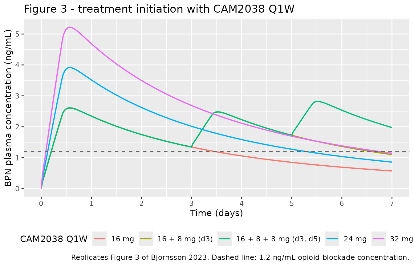
Bjornsson 2023 Results 3.2 states that “BPN concentrations of 1.2 ng/mL were reached approximately 5 h after the recommended starting dose of 16 mg CAM2038 Q1W”. The remaining reference values below were read off the published Figure 3 by eye (its axis gridlines resolve to roughly 0.05 ng/mL), so they carry digitisation uncertainty and are a shape check rather than an exact target.
# Values digitised from Figure 3 of Bjornsson 2023 (see caveat above). For the
# titration arms the figure's visually highest late peak is the one following
# the FINAL 8 mg dose, so `peak_from` gives the time of that dose.
fig3_ref <- tibble::tribble(
  ~treatment,                ~peak_from, ~ref_peak, ~ref_day7,
  "16 mg",                            0,      2.63,      0.52,
  "16 + 8 mg (d3)",                  72,      2.50,      1.10,
  "16 + 8 + 8 mg (d3, d5)",         120,      2.82,      1.95,
  "24 mg",                            0,      3.85,      0.79,
  "32 mg",                            0,      5.23,      1.04
)

sim_init |>
  filter(!is.na(Cc)) |>
  left_join(fig3_ref, by = "treatment") |>
  group_by(treatment, peak_from, ref_peak, ref_day7) |>
  summarise(
    last_peak = max(Cc[time >= peak_from[1]]),
    tmax_days = time[which.max(Cc)] / 24,
    `Time to 1.2 ng/mL (h)` = suppressWarnings(min(time[Cc >= 1.2])),
    day7 = Cc[which.min(abs(time - 168))],
    .groups = "drop"
  ) |>
  mutate(treatment = factor(treatment, init_labels)) |>
  arrange(treatment) |>
  select(treatment, last_peak, ref_peak, day7, ref_day7,
         `Time to 1.2 ng/mL (h)`, tmax_days) |>
  rename("CAM2038 Q1W regimen" = treatment,
         "Simulated final peak (ng/mL)" = last_peak,
         "Figure 3 final peak (ng/mL)" = ref_peak,
         "Simulated day 7 (ng/mL)" = day7,
         "Figure 3 day 7 (ng/mL)" = ref_day7,
         "Day-1 Tmax (days)" = tmax_days) |>
  knitr::kable(digits = 3,
               caption = paste("Typical-value initiation metrics versus values",
"digitised from Figure 3 of Bjornsson 2023."))| CAM2038 Q1W regimen | Simulated final peak (ng/mL) | Figure 3 final peak (ng/mL) | Simulated day 7 (ng/mL) | Figure 3 day 7 (ng/mL) | Time to 1.2 ng/mL (h) | Day-1 Tmax (days) |
|---|---|---|---|---|---|---|
| 16 mg | 2.610 | 2.63 | 0.572 | 0.52 | 5.0 | 0.562 |
| 16 + 8 mg (d3) | 2.481 | 2.50 | 1.100 | 1.10 | 5.0 | 0.562 |
| 16 + 8 + 8 mg (d3, d5) | 2.820 | 2.82 | 1.975 | 1.95 | 5.0 | 5.521 |
| 24 mg | 3.915 | 3.85 | 0.858 | 0.79 | 3.5 | 0.562 |
| 32 mg | 5.220 | 5.23 | 1.144 | 1.04 | 2.5 | 0.562 |
Figure 5 - bridging from SL BPN to CAM2038 at steady state
Figure 5 overlays steady-state profiles for the established dose conversions: 16 mg daily SL BPN with 24 mg CAM2038 Q1W (panel a), 16 mg SL with 96 mg CAM2038 Q4W (panel b), and 24 mg Q1W with 96 mg Q4W (panel c). Time is shown relative to the start of the last dosing interval, on the panel’s own interval length.
bridge <- tibble::tribble(
  ~panel,                                  ~treatment,
  "a: 16 mg SL vs 24 mg Q1W",              "SL 16 mg",
  "a: 16 mg SL vs 24 mg Q1W",              "Q1W 24 mg",
  "b: 16 mg SL vs 96 mg Q4W",              "SL 16 mg",
  "b: 16 mg SL vs 96 mg Q4W",              "Q4W 96 mg",
  "c: 24 mg Q1W vs 96 mg Q4W",             "Q1W 24 mg",
  "c: 24 mg Q1W vs 96 mg Q4W",             "Q4W 96 mg"
) |> mutate(treatment = factor(treatment, ss_regimens$label))

sim_ss |>
  filter(!is.na(Cc)) |>
  group_by(treatment, time) |>
  summarise(Q05 = quantile(Cc, 0.05), Q50 = median(Cc), Q95 = quantile(Cc, 0.95),
            .groups = "drop") |>
  group_by(treatment) |>
  mutate(t_rel = (time - min(time)) / 24) |>
  ungroup() |>
  inner_join(bridge, by = "treatment", relationship = "many-to-many") |>
  ggplot(aes(t_rel, Q50, colour = treatment, fill = treatment)) +
  geom_ribbon(aes(ymin = Q05, ymax = Q95), alpha = 0.18, colour = NA) +
  geom_line(linewidth = 0.7) +
  facet_wrap(~panel, scales = "free_x") +
  labs(x = "Time within the steady-state dosing interval (days)",
       y = "BPN plasma concentration (ng/mL)", colour = NULL, fill = NULL,
       title = "Figure 5 - steady-state bridging between SL BPN and CAM2038",
       caption = paste("Replicates Figure 5 of Bjornsson 2023. Line = median,",
                       "band = 5th-95th percentile of 200 simulated subjects.")) +
  theme(legend.position = "bottom")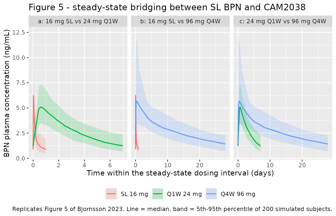
Figure 7 and Table 5 - tapering after interrupting treatment
Figure 7 shows the decline after five doses of CAM2038, and Table 5 reports the geometric-mean time for BPN to fall below 0.1 ng/mL for each Q1W and Q4W dose.
taper_regimens <- tibble::tribble(
  ~label,       ~route, ~dose, ~tau, ~ndose, ~follow_days,
  "16 mg Q1W",  "q1w",    16,   168,      5,   90,
  "24 mg Q1W",  "q1w",    24,   168,      5,   90,
  "32 mg Q1W",  "q1w",    32,   168,      5,   90,
  "64 mg Q4W",  "q4w",    64,   672,      5,  220,
  "96 mg Q4W",  "q4w",    96,   672,      5,  220,
  "128 mg Q4W", "q4w",   128,   672,      5,  220,
  "160 mg Q4W", "q4w",   160,   672,      5,  220
)

taper_events <- dplyr::bind_rows(lapply(seq_len(nrow(taper_regimens)), function(i) {
  r <- taper_regimens[i, ]
  t_last <- r$tau * (r$ndose - 1L)
  make_arm(r$route, r$dose, r$tau, r$ndose,
           obs_time = t_last + seq(0, r$follow_days * 24, by = 12),
           label = r$label, id_offset = (i - 1L) * N_ARM)
}))
stopifnot(!anyDuplicated(unique(taper_events[, c("id", "time", "evid", "cmt")])))

sim_taper <- rxode2::rxSolve(mod, events = taper_events,
                             keep = c("treatment", "route")) |> as.data.frame()
sim_taper |>
  filter(!is.na(Cc), treatment %in% c("32 mg Q1W", "128 mg Q4W")) |>
  group_by(treatment, time) |>
  summarise(Q025 = quantile(Cc, 0.025), Q50 = median(Cc),
            Q975 = quantile(Cc, 0.975), .groups = "drop") |>
  group_by(treatment) |>
  mutate(days_after_last = (time - min(time)) / 24) |>
  ungroup() |>
  ggplot(aes(days_after_last, Q50)) +
  geom_ribbon(aes(ymin = Q025, ymax = Q975), alpha = 0.2) +
  geom_line(linewidth = 0.7) +
  geom_hline(yintercept = 0.1, linetype = "dashed", colour = "firebrick") +
  facet_wrap(~treatment, scales = "free_x") +
  scale_y_log10() +
  labs(x = "Days after the last dose", y = "BPN plasma concentration (ng/mL)",
       title = "Figure 7 - decline after five doses of CAM2038",
       caption = paste("Replicates Figure 7 of Bjornsson 2023. Dashed line:",
                       "the 0.1 ng/mL threshold used in Table 5."))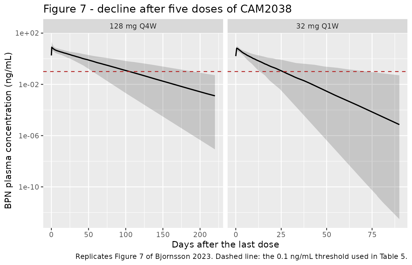
gm <- function(x) exp(mean(log(x)))

taper_pub <- tibble::tribble(
  ~treatment,   ~pub_gm, ~pub_lo, ~pub_hi,
  "16 mg Q1W",     21.8,    10.9,    52.3,
  "24 mg Q1W",     25.6,    12.0,    60.9,
  "32 mg Q1W",     27.3,    13.0,    63.1,
  "64 mg Q4W",     82.3,    43.9,     150,
  "96 mg Q4W",     92.9,    50.4,     165,
  "128 mg Q4W",     101,    55.4,     183,
  "160 mg Q4W",     104,    56.9,     192
)

# Last time at or above 0.1 ng/mL; the next grid point is the first sustained
# time below the threshold. Concentrations decline monotonically over the
# follow-up window, so this is the crossing time to grid resolution (12 h).
first_below <- function(time, Cc, thresh = 0.1) {
  o <- order(time)
  time <- time[o]; Cc <- Cc[o]
  if (all(Cc < thresh)) return(0)
  if (Cc[length(Cc)] >= thresh) return(NA_real_)
  (time[max(which(Cc >= thresh)) + 1L] - time[1]) / 24
}

sim_taper |>
  filter(!is.na(Cc)) |>
  group_by(treatment, id) |>
  summarise(t_below = first_below(time, Cc), .groups = "drop") |>
  group_by(treatment) |>
  summarise(n_reached = sum(!is.na(t_below)),
            sim_gm = gm(t_below[!is.na(t_below)]),
            sim_lo = quantile(t_below, 0.025, na.rm = TRUE),
            sim_hi = quantile(t_below, 0.975, na.rm = TRUE), .groups = "drop") |>
  left_join(taper_pub, by = "treatment") |>
  mutate(`% diff` = 100 * (sim_gm - pub_gm) / pub_gm,
         treatment = factor(treatment, taper_regimens$label)) |>
  arrange(treatment) |>
  select(treatment, sim_gm, pub_gm, `% diff`, sim_lo, sim_hi, pub_lo, pub_hi) |>
  rename("Regimen" = treatment,
         "Simulated geo. mean (d)" = sim_gm, "Paper geo. mean (d)" = pub_gm,
         "Simulated 2.5th (d)" = sim_lo, "Simulated 97.5th (d)" = sim_hi,
         "Paper 95% PI low (d)" = pub_lo, "Paper 95% PI high (d)" = pub_hi) |>
  knitr::kable(digits = 1,
               caption = paste("Table 5 of Bjornsson 2023 - days for BPN to fall",
"below 0.1 ng/mL after five CAM2038 doses."))| Regimen | Simulated geo. mean (d) | Paper geo. mean (d) | % diff | Simulated 2.5th (d) | Simulated 97.5th (d) | Paper 95% PI low (d) | Paper 95% PI high (d) |
|---|---|---|---|---|---|---|---|
| 16 mg Q1W | 22.8 | 21.8 | 4.4 | 11.0 | 54.2 | 10.9 | 52.3 |
| 24 mg Q1W | 25.5 | 25.6 | -0.5 | 12.5 | 56.1 | 12.0 | 60.9 |
| 32 mg Q1W | 27.0 | 27.3 | -1.0 | 13.5 | 66.3 | 13.0 | 63.1 |
| 64 mg Q4W | 79.7 | 82.3 | -3.1 | 46.0 | 165.7 | 43.9 | 150.0 |
| 96 mg Q4W | 95.7 | 92.9 | 3.0 | 53.9 | 183.1 | 50.4 | 165.0 |
| 128 mg Q4W | 104.6 | 101.0 | 3.6 | 55.9 | 184.2 | 55.4 | 183.0 |
| 160 mg Q4W | 105.3 | 104.0 | 1.2 | 51.4 | 186.3 | 56.9 | 192.0 |
PKNCA validation
Steady-state NCA is computed on the final dosing interval of each regimen, with the treatment label as the grouping variable so results can be compared with Table 4 per regimen.
The paper’s Ctrough,ss is taken from PKNCA’s
cmin over the steady-state interval rather than
ctrough: these profiles decline monotonically from their
peak to the end of the interval, so the interval minimum is the
trough (for the Q1W 16 mg arm the two agree to four significant
figures), and PKNCA’s ctrough returns NA in
this configuration. The Cmax,ss / Ctrough,ss ratio is
therefore formed per subject as cmax / cmin and then
aggregated, rather than taken from PKNCA’s ptr.
sim_nca <- sim_ss |>
  dplyr::filter(!is.na(Cc)) |>
  dplyr::select(id, time, Cc, treatment)

dose_df <- ss_events |>
  dplyr::filter(evid == 1, cmt %in% c("depot_sl1", "depot_q1w1", "depot_q4w1")) |>
  dplyr::select(id, time, amt, treatment, tau, ii, addl) |>
  dplyr::mutate(time = time + ii * addl) |>   # the final dose of the regimen
  dplyr::select(id, time, amt, treatment)

conc_obj <- PKNCA::PKNCAconc(sim_nca, Cc ~ time | treatment + id,
                             concu = "ng/mL", timeu = "hr")
dose_obj <- PKNCA::PKNCAdose(dose_df, amt ~ time | treatment + id,
                             doseu = "mg")

# One steady-state interval per regimen: [last dose, last dose + tau].
intervals <- ss_regimens |>
  transmute(start = tau * (ndose - 1L), end = start + tau,
            treatment = factor(label, ss_regimens$label),
            cmax = TRUE, tmax = TRUE, cav = TRUE, cmin = TRUE,
            auclast = TRUE) |>
  as.data.frame()

nca_res <- PKNCA::pk.nca(
  PKNCA::PKNCAdata(conc_obj, dose_obj, intervals = intervals)
)

# Per-subject metrics, with the peak-to-trough ratio derived from cmax / cmin.
gcv <- function(x) 100 * sqrt(exp(stats::var(log(x))) - 1)

nca_subj <- as.data.frame(nca_res) |>
  filter(PPTESTCD %in% c("cmax", "cav", "cmin"), !is.na(PPORRES)) |>
  select(treatment, id, PPTESTCD, PPORRES) |>
  tidyr::pivot_wider(names_from = PPTESTCD, values_from = PPORRES) |>
  mutate(ptr = cmax / cmin) |>
  tidyr::pivot_longer(c(cmax, cav, cmin, ptr),
                      names_to = "PPTESTCD", values_to = "PPORRES")
Comparison against published Table 4
Table 4 reports geometric means (with geometric CV
%), so the per-subject PKNCA output is aggregated with the geometric
mean rather than ncaComparisonTable()’s default median.
sim_wide <- nca_subj |>
  group_by(treatment, PPTESTCD) |>
  summarise(PPORRES = gm(PPORRES), .groups = "drop") |>
  tidyr::pivot_wider(names_from = PPTESTCD, values_from = PPORRES) |>
  mutate(treatment = as.character(treatment))

published <- tibble::tribble(
  ~treatment,   ~cmax, ~cav,  ~cmin,  ~ptr,
  "SL 8 mg",     3.92, 1.08,  0.540,  7.26,
  "SL 16 mg",    6.09, 1.69,  0.852,  7.15,
  "SL 24 mg",    7.94, 2.21,  1.10,   7.24,
  "Q1W 8 mg",    1.69, 0.893, 0.386,  4.37,
  "Q1W 16 mg",   3.38, 1.79,  0.780,  4.34,
  "Q1W 24 mg",   4.97, 2.66,  1.18,   4.21,
  "Q1W 32 mg",   6.75, 3.57,  1.55,   4.37,
  "Q4W 64 mg",   4.11, 1.83,  0.870,  4.72,
  "Q4W 96 mg",   5.84, 2.71,  1.34,   4.36,
  "Q4W 128 mg",  8.16, 3.68,  1.74,   4.69,
  "Q4W 160 mg",  9.97, 4.52,  2.21,   4.52
)

cmp <- nlmixr2lib::ncaComparisonTable(
  simulated = sim_wide,
  reference = published,
  by        = "treatment",
  units     = c(cmax = "ng/mL", cav = "ng/mL", cmin = "ng/mL",
                ptr = "Cmax,ss / Ctrough,ss"),
  tolerance_pct = 20
)

cmp |>
  mutate(treatment = factor(treatment, ss_regimens$label)) |>
  arrange(treatment) |>
  rename("Regimen" = treatment) |>
  knitr::kable(
    digits = 3,
    caption = paste("Simulated vs. published steady-state NCA (Table 4 of",
                    "Bjornsson 2023). * differs from the paper by > 20 %.")
)| NCA parameter | Regimen | Reference | Simulated | % diff |
|---|---|---|---|---|
| Cmax (ng/mL) | SL 8 mg | 3.92 | 4.17 | +6.4% |
| Cmin (ng/mL) | SL 8 mg | 0.54 | 0.601 | +11.4% |
| Cavg (ng/mL) | SL 8 mg | 1.08 | 1.16 | +7.8% |
| PTR (Cmax,ss / Ctrough,ss) | SL 8 mg | 7.26 | 6.94 | -4.5% |
| Cmax (ng/mL) | SL 16 mg | 6.09 | 6.55 | +7.5% |
| Cmin (ng/mL) | SL 16 mg | 0.852 | 0.898 | +5.4% |
| Cavg (ng/mL) | SL 16 mg | 1.69 | 1.76 | +4.2% |
| PTR (Cmax,ss / Ctrough,ss) | SL 16 mg | 7.15 | 7.29 | +1.9% |
| Cmax (ng/mL) | SL 24 mg | 7.94 | 8.26 | +4.1% |
| Cmin (ng/mL) | SL 24 mg | 1.1 | 1.21 | +9.6% |
| Cavg (ng/mL) | SL 24 mg | 2.21 | 2.3 | +3.9% |
| PTR (Cmax,ss / Ctrough,ss) | SL 24 mg | 7.24 | 6.85 | -5.4% |
| Cmax (ng/mL) | Q1W 8 mg | 1.69 | 1.64 | -2.8% |
| Cmin (ng/mL) | Q1W 8 mg | 0.386 | 0.401 | +3.8% |
| Cavg (ng/mL) | Q1W 8 mg | 0.893 | 0.89 | -0.4% |
| PTR (Cmax,ss / Ctrough,ss) | Q1W 8 mg | 4.37 | 4.1 | -6.2% |
| Cmax (ng/mL) | Q1W 16 mg | 3.38 | 3.44 | +1.7% |
| Cmin (ng/mL) | Q1W 16 mg | 0.78 | 0.825 | +5.8% |
| Cavg (ng/mL) | Q1W 16 mg | 1.79 | 1.85 | +3.6% |
| PTR (Cmax,ss / Ctrough,ss) | Q1W 16 mg | 4.34 | 4.16 | -4.1% |
| Cmax (ng/mL) | Q1W 24 mg | 4.97 | 5.09 | +2.4% |
| Cmin (ng/mL) | Q1W 24 mg | 1.18 | 1.23 | +4.5% |
| Cavg (ng/mL) | Q1W 24 mg | 2.66 | 2.76 | +3.8% |
| PTR (Cmax,ss / Ctrough,ss) | Q1W 24 mg | 4.21 | 4.13 | -2.0% |
| Cmax (ng/mL) | Q1W 32 mg | 6.75 | 6.73 | -0.3% |
| Cmin (ng/mL) | Q1W 32 mg | 1.55 | 1.64 | +6.0% |
| Cavg (ng/mL) | Q1W 32 mg | 3.57 | 3.6 | +0.8% |
| PTR (Cmax,ss / Ctrough,ss) | Q1W 32 mg | 4.37 | 4.1 | -6.2% |
| Cmax (ng/mL) | Q4W 64 mg | 4.11 | 4 | -2.6% |
| Cmin (ng/mL) | Q4W 64 mg | 0.87 | 0.909 | +4.5% |
| Cavg (ng/mL) | Q4W 64 mg | 1.83 | 1.85 | +1.3% |
| PTR (Cmax,ss / Ctrough,ss) | Q4W 64 mg | 4.72 | 4.4 | -6.7% |
| Cmax (ng/mL) | Q4W 96 mg | 5.84 | 6 | +2.7% |
| Cmin (ng/mL) | Q4W 96 mg | 1.34 | 1.33 | -0.5% |
| Cavg (ng/mL) | Q4W 96 mg | 2.71 | 2.73 | +0.9% |
| PTR (Cmax,ss / Ctrough,ss) | Q4W 96 mg | 4.36 | 4.5 | +3.2% |
| Cmax (ng/mL) | Q4W 128 mg | 8.16 | 7.63 | -6.5% |
| Cmin (ng/mL) | Q4W 128 mg | 1.74 | 1.74 | -0.1% |
| Cavg (ng/mL) | Q4W 128 mg | 3.68 | 3.62 | -1.6% |
| PTR (Cmax,ss / Ctrough,ss) | Q4W 128 mg | 4.69 | 4.39 | -6.3% |
| Cmax (ng/mL) | Q4W 160 mg | 9.97 | 9.72 | -2.5% |
| Cmin (ng/mL) | Q4W 160 mg | 2.21 | 2.26 | +2.4% |
| Cavg (ng/mL) | Q4W 160 mg | 4.52 | 4.61 | +2.0% |
| PTR (Cmax,ss / Ctrough,ss) | Q4W 160 mg | 4.52 | 4.29 | -5.0% |
The paper’s own geometric CV percentages are the sharpest available
check on how the Table 3 IIV / CV (%) column should be read
(see Assumptions below), so they are compared as well.
published_cv <- tibble::tribble(
  ~treatment,   ~cmax, ~cav, ~cmin, ~ptr,
  "SL 8 mg",       37,   33,    46,   46,
  "SL 16 mg",      36,   33,    45,   44,
  "SL 24 mg",      38,   35,    47,   45,
  "Q1W 8 mg",      25,   22,    45,   54,
  "Q1W 16 mg",     24,   22,    45,   53,
  "Q1W 24 mg",     25,   21,    45,   55,
  "Q1W 32 mg",     24,   21,    43,   52,
  "Q4W 64 mg",     41,   21,    40,   66,
  "Q4W 96 mg",     35,   20,    33,   52,
  "Q4W 128 mg",    40,   22,    39,   63,
  "Q4W 160 mg",    39,   22,    39,   60
) |> tidyr::pivot_longer(-treatment, names_to = "PPTESTCD", values_to = "paper_cv")

cv_cmp <- nca_subj |>
  group_by(treatment, PPTESTCD) |>
  summarise(sim_cv = gcv(PPORRES), .groups = "drop") |>
  mutate(treatment = as.character(treatment)) |>
  left_join(published_cv, by = c("treatment", "PPTESTCD")) |>
  mutate(diff_pp = sim_cv - paper_cv,
         label = dplyr::recode(PPTESTCD, cmax = "Cmax,ss", cav = "Cav,ss",
                               cmin = "Ctrough,ss", ptr = "Cmax,ss/Ctrough,ss"),
         treatment = factor(treatment, ss_regimens$label))

cv_cmp |>
  select(treatment, label, sim_cv, paper_cv, diff_pp) |>
  arrange(treatment, label) |>
  rename("Regimen" = treatment, "NCA parameter" = label,
         "Simulated geo. CV (%)" = sim_cv, "Paper geo. CV (%)" = paper_cv,
         "Difference (pp)" = diff_pp) |>
  knitr::kable(digits = 1,
               caption = paste("Geometric CV percentages, simulated vs. Table 4",
"of Bjornsson 2023 (pp = percentage points)."))| Regimen | NCA parameter | Simulated geo. CV (%) | Paper geo. CV (%) | Difference (pp) |
|---|---|---|---|---|
| SL 8 mg | Cav,ss | 34.4 | 33 | 1.4 |
| SL 8 mg | Cmax,ss | 37.3 | 37 | 0.3 |
| SL 8 mg | Cmax,ss/Ctrough,ss | 45.4 | 46 | -0.6 |
| SL 8 mg | Ctrough,ss | 45.5 | 46 | -0.5 |
| SL 16 mg | Cav,ss | 36.6 | 33 | 3.6 |
| SL 16 mg | Cmax,ss | 37.3 | 36 | 1.3 |
| SL 16 mg | Cmax,ss/Ctrough,ss | 39.1 | 44 | -4.9 |
| SL 16 mg | Ctrough,ss | 48.1 | 45 | 3.1 |
| SL 24 mg | Cav,ss | 35.8 | 35 | 0.8 |
| SL 24 mg | Cmax,ss | 38.4 | 38 | 0.4 |
| SL 24 mg | Cmax,ss/Ctrough,ss | 42.5 | 45 | -2.5 |
| SL 24 mg | Ctrough,ss | 45.7 | 47 | -1.3 |
| Q1W 8 mg | Cav,ss | 22.5 | 22 | 0.5 |
| Q1W 8 mg | Cmax,ss | 26.1 | 25 | 1.1 |
| Q1W 8 mg | Cmax,ss/Ctrough,ss | 56.1 | 54 | 2.1 |
| Q1W 8 mg | Ctrough,ss | 46.6 | 45 | 1.6 |
| Q1W 16 mg | Cav,ss | 21.5 | 22 | -0.5 |
| Q1W 16 mg | Cmax,ss | 24.2 | 24 | 0.2 |
| Q1W 16 mg | Cmax,ss/Ctrough,ss | 53.6 | 53 | 0.6 |
| Q1W 16 mg | Ctrough,ss | 45.7 | 45 | 0.7 |
| Q1W 24 mg | Cav,ss | 21.6 | 21 | 0.6 |
| Q1W 24 mg | Cmax,ss | 23.5 | 25 | -1.5 |
| Q1W 24 mg | Cmax,ss/Ctrough,ss | 50.0 | 55 | -5.0 |
| Q1W 24 mg | Ctrough,ss | 43.2 | 45 | -1.8 |
| Q1W 32 mg | Cav,ss | 21.8 | 21 | 0.8 |
| Q1W 32 mg | Cmax,ss | 24.7 | 24 | 0.7 |
| Q1W 32 mg | Cmax,ss/Ctrough,ss | 46.8 | 52 | -5.2 |
| Q1W 32 mg | Ctrough,ss | 40.9 | 43 | -2.1 |
| Q4W 64 mg | Cav,ss | 19.9 | 21 | -1.1 |
| Q4W 64 mg | Cmax,ss | 37.6 | 41 | -3.4 |
| Q4W 64 mg | Cmax,ss/Ctrough,ss | 59.6 | 66 | -6.4 |
| Q4W 64 mg | Ctrough,ss | 36.5 | 40 | -3.5 |
| Q4W 96 mg | Cav,ss | 20.6 | 20 | 0.6 |
| Q4W 96 mg | Cmax,ss | 39.7 | 35 | 4.7 |
| Q4W 96 mg | Cmax,ss/Ctrough,ss | 59.4 | 52 | 7.4 |
| Q4W 96 mg | Ctrough,ss | 37.2 | 33 | 4.2 |
| Q4W 128 mg | Cav,ss | 19.7 | 22 | -2.3 |
| Q4W 128 mg | Cmax,ss | 37.5 | 40 | -2.5 |
| Q4W 128 mg | Cmax,ss/Ctrough,ss | 63.2 | 63 | 0.2 |
| Q4W 128 mg | Ctrough,ss | 37.6 | 39 | -1.4 |
| Q4W 160 mg | Cav,ss | 20.7 | 22 | -1.3 |
| Q4W 160 mg | Cmax,ss | 37.8 | 39 | -1.2 |
| Q4W 160 mg | Cmax,ss/Ctrough,ss | 51.9 | 60 | -8.1 |
| Q4W 160 mg | Ctrough,ss | 30.4 | 39 | -8.6 |
cv_cmp |>
  group_by(`NCA parameter` = label) |>
  summarise(`Mean |difference| (pp)` = mean(abs(diff_pp)),
            `Max |difference| (pp)` = max(abs(diff_pp)), .groups = "drop") |>
  knitr::kable(digits = 2,
               caption = paste("Aggregate agreement of the simulated geometric",
"CV percentages with Table 4."))| NCA parameter | Mean |difference| (pp) | Max |difference| (pp) |
|---|---|---|
| Cav,ss | 1.23 | 3.65 |
| Cmax,ss | 1.57 | 4.69 |
| Cmax,ss/Ctrough,ss | 3.91 | 8.14 |
| Ctrough,ss | 2.61 | 8.61 |
Which reading of the Table 3 IIV / CV (%) column?
Table 3 reports a single CV (%) column spanning both
exponentially distributed parameters and the four logit-transformed
fractions. A coefficient of variation is undefined for a logit-normal
parameter, so the column can only be uniform if it carries
100 * omega - the standard deviation of eta on the
transformed scale. The model file adopts that reading
(variance = (CV / 100)^2); the alternative log-normal
reading is omega^2 = log(1 + CV^2).
The choice is testable, because Table 4’s geometric CV percentages are a direct readout of the omegas. The block below re-solves every regimen under the alternative reading and scores both against Table 4. Nothing here is fitted - the published CVs are recovered from the model’s own OMEGA diagonal, so the two matrices are two deterministic transforms of the same 11 published numbers.
omega_adopted <- rxode2::rxode2(mod)$omega
#> ℹ parameter labels from comments will be replaced by 'label()'
cv_published  <- sqrt(diag(omega_adopted))     # recovers the Table 3 CV/100
omega_alt     <- diag(log(1 + cv_published^2))
dimnames(omega_alt) <- dimnames(omega_adopted)

# Same NCA pipeline, driven by a supplied OMEGA.
cv_under <- function(omega) {
  s <- rxode2::rxSolve(mod, events = ss_events, omega = omega,
                       keep = "treatment") |> as.data.frame()
  nc <- s |> filter(!is.na(Cc)) |> select(id, time, Cc, treatment)
  r <- PKNCA::pk.nca(PKNCA::PKNCAdata(
    PKNCA::PKNCAconc(nc, Cc ~ time | treatment + id,
                     concu = "ng/mL", timeu = "hr"),
    dose_obj, intervals = intervals))
  as.data.frame(r) |>
    filter(PPTESTCD %in% c("cmax", "cav", "cmin"), !is.na(PPORRES)) |>
    select(treatment, id, PPTESTCD, PPORRES) |>
    tidyr::pivot_wider(names_from = PPTESTCD, values_from = PPORRES) |>
    mutate(ptr = cmax / cmin) |>
    tidyr::pivot_longer(c(cmax, cav, cmin, ptr),
                        names_to = "PPTESTCD", values_to = "PPORRES") |>
    group_by(treatment, PPTESTCD) |>
    summarise(sim_cv = gcv(PPORRES), .groups = "drop") |>
    mutate(treatment = as.character(treatment))
}

bind_rows(
  cv_under(omega_adopted) |> mutate(reading = "Adopted: var = (CV/100)^2"),
  cv_under(omega_alt)     |> mutate(reading = "Alternative: var = log(1 + CV^2)")
) |>
  left_join(published_cv, by = c("treatment", "PPTESTCD")) |>
  mutate(label = dplyr::recode(PPTESTCD, cmax = "Cmax,ss", cav = "Cav,ss",
                               cmin = "Ctrough,ss",
                               ptr = "Cmax,ss/Ctrough,ss")) |>
  group_by(reading, label) |>
  summarise(bias = mean(sim_cv - paper_cv),
            mae = mean(abs(sim_cv - paper_cv)), .groups = "drop") |>
  tidyr::pivot_longer(c(bias, mae), names_to = "stat", values_to = "pp") |>
  mutate(stat = dplyr::recode(stat, bias = "Mean signed diff.",
                              mae = "Mean |diff.|")) |>
  tidyr::pivot_wider(names_from = reading, values_from = pp) |>
  arrange(label, stat) |>
  rename("NCA parameter" = label, "Statistic" = stat) |>
  knitr::kable(digits = 2,
               caption = paste("Deviation (percentage points) of the simulated",
                               "geometric CV from Table 4 under the two readings",
                               "of the Table 3 IIV column, across all 11",
                               "regimens. A negative signed difference means the",
"simulated variability is too narrow."))| NCA parameter | Statistic | Adopted: var = (CV/100)^2 | Alternative: var = log(1 + CV^2) |
|---|---|---|---|
| Cav,ss | Mean signed diff. | -0.71 | 0.34 |
| Cav,ss | Mean |diff.| | 1.30 | 1.29 |
| Cmax,ss | Mean signed diff. | -1.12 | -2.37 |
| Cmax,ss | Mean |diff.| | 2.71 | 2.97 |
| Cmax,ss/Ctrough,ss | Mean signed diff. | -1.31 | -6.51 |
| Cmax,ss/Ctrough,ss | Mean |diff.| | 4.91 | 6.85 |
| Ctrough,ss | Mean signed diff. | -0.78 | -1.78 |
| Ctrough,ss | Mean |diff.| | 3.18 | 2.44 |
Covariate effects
The final model retained age and body weight on CL, OUD status on Vc,
and OUD status and female sex on Fq1w1. The demographic
cohort below illustrates them for 24 mg CAM2038 Q1W at steady state.
Fq1w1 redistributes dose between the fast and slow
pathways, so it moves Cmax and Ctrough in
opposite directions while leaving overall exposure (AUC,
hence Cav) unchanged - the point made in Results 3.1.3 and
Discussion 4.1.
cov_arms <- tibble::tribble(
  ~label,                        ~age, ~wt, ~sexf, ~oud, ~thigh,
  "Reference (healthy M, 35 y, 72.4 kg)", 35, 72.4,  0,    0,     0,
  "Female",                               35, 72.4,  1,    0,     0,
  "OUD",                                  35, 72.4,  0,    1,     0,
  "Age 65 y",                             65, 72.4,  0,    0,     0,
  "Weight 100 kg",                        35,  100,  0,    0,     0,
  "Thigh injection",                      35, 72.4,  0,    0,     1
)

cov_events <- dplyr::bind_rows(lapply(seq_len(nrow(cov_arms)), function(i) {
  a <- cov_arms[i, ]
  make_arm("q1w", 24, 168, 12, obs_time = seq(1848, 2016, by = 2),
           label = a$label, id_offset = (i - 1L) * N_ARM,
           age = a$age, wt = a$wt, sexf = a$sexf, oud = a$oud, thigh = a$thigh)
}))
stopifnot(!anyDuplicated(unique(cov_events[, c("id", "time", "evid", "cmt")])))

sim_cov <- rxode2::rxSolve(mod, events = cov_events, keep = "treatment") |>
  as.data.frame()

sim_cov |>
  filter(!is.na(Cc)) |>
  group_by(treatment, id) |>
  summarise(cmax = max(Cc), ctrough = Cc[which.max(time)],
            cav = sum(diff(time) * (head(Cc, -1) + tail(Cc, -1)) / 2) /
              (max(time) - min(time)), .groups = "drop") |>
  group_by(treatment) |>
  summarise(across(c(cmax, cav, ctrough), gm), .groups = "drop") |>
  mutate(treatment = factor(treatment, cov_arms$label)) |>
  arrange(treatment) |>
  rename("Covariate scenario" = treatment, "Cmax,ss (ng/mL)" = cmax,
         "Cav,ss (ng/mL)" = cav, "Ctrough,ss (ng/mL)" = ctrough) |>
  knitr::kable(digits = 3,
               caption = paste("Retained covariate effects at steady state on",
                               "24 mg CAM2038 Q1W (geometric means, n = 200",
"per scenario)."))| Covariate scenario | Cmax,ss (ng/mL) | Cav,ss (ng/mL) | Ctrough,ss (ng/mL) |
|---|---|---|---|
| Reference (healthy M, 35 y, 72.4 kg) | 5.172 | 2.758 | 1.212 |
| Female | 5.622 | 2.749 | 1.041 |
| OUD | 4.324 | 2.686 | 1.452 |
| Age 65 y | 5.634 | 3.140 | 1.443 |
| Weight 100 kg | 4.837 | 2.493 | 1.072 |
| Thigh injection | 3.296 | 2.716 | 1.849 |
sim_cov |>
  filter(!is.na(Cc)) |>
  group_by(treatment, time) |>
  summarise(Q50 = median(Cc), .groups = "drop") |>
  group_by(treatment) |>
  mutate(t_rel = (time - min(time)) / 24) |>
  ungroup() |>
  mutate(treatment = factor(treatment, cov_arms$label)) |>
  ggplot(aes(t_rel, Q50, colour = treatment)) +
  geom_line(linewidth = 0.7) +
  labs(x = "Time within the steady-state weekly interval (days)",
       y = "Median BPN plasma concentration (ng/mL)", colour = NULL,
       title = "Retained covariate effects, 24 mg CAM2038 Q1W at steady state") +
  theme(legend.position = "bottom")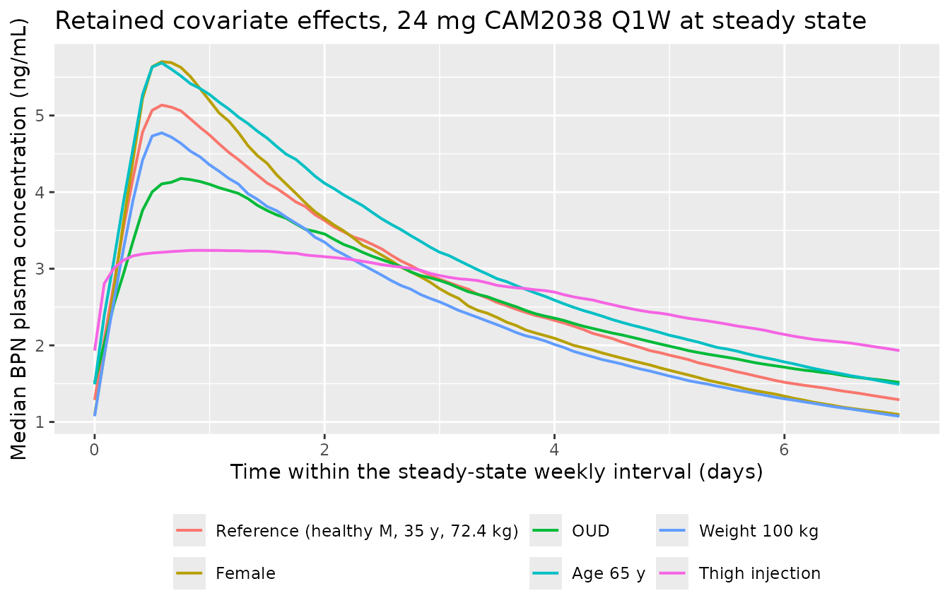
Assumptions and deviations
-
How the Table 3
IIV / CV (%)column is read. Table 3 reports oneCV (%)column spanning both exponentially distributed parameters (Methods Eq. 1) and logit-transformed parameters (F_SL,F_SL1,Fq1w1,Fq4w1; Methods Eqs. 2-3). A coefficient of variation is undefined for a logit-normal parameter, so a single column can only be uniform if it carries100 * omega, the standard deviation of eta on the transformed scale. The model file therefore encodesvariance = (CV / 100)^2. The “Which reading of the Table 3IIV / CV (%)column?” section above tests this against the paper’s own geometric CV percentages across all 11 regimens of Table 4. The adopted reading wins overall, and the discriminating quantity is theCmax,ss / Ctrough,ssratio CV - the metric most sensitive to the large logit-scale etas onFq1w1andFq4w1- where the log-normal alternativeomega^2 = log(1 + CV^2)is systematically too narrow. The two readings differ by under 1.5 % relative for the exponentially distributed parameters (omega= 0.209 versus 0.2068 for CL, for instance), so the choice materially affects only the four logit-transformed fractions, where the gap is larger (0.921 versus 0.785 forFq4w1). At the 200-subjects-per-arm cohort size used here the margin between the two readings is modest relative to Monte Carlo noise on a CV; a higher-powered run of the same comparison at 1000 per arm (the paper’s replicate count, above this vignette’s cohort cap) separates them more cleanly, at 1.8 versus 2.7 percentage points of mean absolute error over the same 44 targets. -
Where the IIV on
F_SLenters relative to the dose effect. Methods Eq. 2 applies the logit transform to “the typical parameter value (P)”, and Results 3.1.3 prints the typical value as the dose-dependentF_SL = 0.14 * (Dose/16)^-0.371. The model file therefore adds eta to the logit of the dose-adjusted typical value, which keeps every individualF_SLinside (0, 1). Applying eta to the logit of the 16 mg value and then scaling by the dose term is numerically identical at the 16 mg reference dose and differs only in how variability propagates at other doses; it is not used here because it can push an individualF_SLabove 1. -
The printed
F_SLequation is a power model, contradicting Methods Eq. 4. Eq. 4 states that continuous covariates enter “as power models for untransformed parameters and linear models for logit-transformed parameters”, which for the logit-transformedF_SLwould mean an additive shift of-0.371 * log(Dose/16)on the logit scale. That form givesF_SL(8 mg) = 17.4 %, not the 18.1 % the paper itself reports. The power form printed in Results 3.1.3 reproduces all three published values (18.1 / 14.0 / 12.0 % at 8 / 16 / 24 mg) exactly, so the printed equation is used and the Methods generalisation is treated as not applying to this term. -
Categorical covariates on
Fq1w1are additive on the logit scale. Methods Eq. 5 describes categorical covariates as “a fractional difference to the most common category”, which for an untransformed parameter such asVcmeansVc * (1 + theta)- that form reproduces the published 64.3 L (healthy) versus 237 L (OUD) exactly and is what the model file uses. Applying the same multiplicative form tologit(Fq1w1)would makeFq1w1higher in participants with OUD (48.5 %) and lower in women (42.9 %), contradicting Results 3.1.3 (“HigherFq1w1was shown in women than in men, and in healthy individuals versus those with OUD”). Adding the coefficients on the logit scale gives 29.9 % for OUD and 59.8 % for women, matching both stated directions. The additive-on-logit reading is therefore used; the paper does not print theFq1w1covariate equation explicitly. -
Fq4w1= 8.63 % (Table 3) versus 0.0900 implied in the text. Results 3.1.3 writes the slow-pathway Q4W fraction as “0.910 (= 1 - 0.0900)”, while Table 3 reportsFq4w1 = 8.63 %. The Table 3 value is used, being the final model’s parameter table; it reproduces the paper’s “70.1 % of the CAM2038 Q4W dose was absorbed after 28 days” as 70.05 % (the text’s 0.0900 gives 70.17 %). -
Injection-site typo in Results 3.1.1. The sentence
“for injections in the thigh, the entire dose was absorbed through the
slower of the two absorption pathways (
ka,q1w1) with the estimated dose fraction entering compartment q1w1 (Fq1w1) close to 0” nameska,q1w1as the slower pathway, butka,q1w1= 0.0401 1/h is the faster of the Q1W pair andFq1w1= 0 routes the dose intodepot_q1w2(ka,q1w2= 0.00565 1/h). Results 3.1.3 and Discussion 4.1 both confirmka,q1w2is the slow pathway. The model implementsFq1w1 = 0for thigh injections, which sends the whole dose throughdepot_q1w2, consistent with the rest of the paper. - Covariates in the replication cohort are fixed, not sampled. Methods 2.4 states the paper’s simulations were for a typical healthy 35-year-old, 72.4 kg male. The Table 4 / Table 5 replications hold covariates at those values so only inter-individual random effects vary, matching the published design. The covariate-effect section uses a separate scenario cohort instead of a sampled demographic distribution, because the paper reports covariate effects as point-value contrasts rather than as a distributional summary.
- Cohort size. 200 subjects per arm (the nlmixr2lib cap) versus the paper’s 1000 replicates. With geometric CVs of 20-66 %, the Monte Carlo standard error on a simulated geometric mean is roughly 1.5-4.5 % at n = 200, and on a simulated geometric CV roughly 1-3 percentage points. That is the floor on the agreement achievable in the comparison tables, and it is the reason the IIV-reading discriminator above is less sharp here than at the paper’s n.
-
Steady state. Dose counts (20 daily SL, 12 weekly,
10 monthly) were chosen from a typical-value convergence check rather
than taken from the paper, which states only that “steady-state
conditions appear to be reached within 4 doses” of CAM2038 and within 7
daily SL doses. At 4 weekly doses the typical-value
Cav,ssis 1.6 % below its converged value, so the paper’s own simulations may sit marginally below full steady state. - Tapering setup. Table 5 describes decay “after interrupting treatment with CAM2038 at steady state” while Figure 7 specifies five doses. Five doses are used here, matching Figure 7’s explicit design. Note also that Table 5’s “Geometric CV %” column (1.33-1.82) is not a percentage - the values are consistent with a geometric standard deviation, not a CV, given the published 95 % prediction intervals span 3- to 5-fold.
-
Sublingual concentrations run high; CAM2038 does
not. Simulated SL
Cmax,ss,Cav,ss, andCtrough,ssexceed Table 4 by 4-11 % at all three doses, all in the same direction, whereas the CAM2038 Q1W and Q4W regimens straddle the published values (-6.5 % to +3.6 %). The SL shape is right - theCmax,ss / Ctrough,ssratio is within 6 % and every SL geometric CV within 5 percentage points - so the residual is a level offset on the SL bioavailable dose rather than a structural error in the dual SL absorption pathway. No reported quantity in the paper distinguishes its cause, and nothing was tuned. Note that the paper independently reports its own model-predicted SL steady-state values as running below the observed non-compartmental values (Discussion 4.1), so its published SL simulation is known to sit at the low end. All 44 Table 4 targets are within 12 %, well inside the 20 % flag threshold, so no row is starred. -
Residual error. Results 3.1.1 describes the RUV as
additive on log-transformed concentrations, which is proportional on the
linear scale; Table 3 reports it directly as
sigma_prop= 27.7 %, encoded aspropSd = 0.277. - No parameter uncertainty. The simulations propagate inter-individual variability only. Table 3’s relative standard errors are recorded in the model file’s in-file comments but no covariance matrix is published, so parameter uncertainty is not propagated (the paper’s own prediction intervals likewise reflect IIV).
-
Compartment naming. The six absorption depots use
the source paper’s own Figure 1 labels (
depot_sl1,depot_sl2,depot_q1w1,depot_q1w2,depot_q4w1,depot_q4w2) and are declared through the model file’spaper_specific_compartmentsfield. Four of the six name pathways of two proprietary CAM2038 formulations and so were not registered as new canonical compartments; the generic blesseddepot1…depot6numbering was rejected because a user dosing this four-route model must be able to tell which depot pair belongs to which formulation and which member is the fast pathway. -
New canonical covariates.
DIS_OUD(opioid use disorder indicator) andDOSE_BPN_SL_MG(administered sublingual dose, needed becausemodel()code cannot read theamtof the dose record it scales) were added toinst/references/covariate-columns.mdin the same change.INJSITE_THIGHalready existed and gained this model in its example list. -
Not implemented: BLQ handling and the 192 mg Q4W
dose. Concentrations below the 0.0250 ng/mL LLOQ were excluded
from the paper’s estimation but retained for its visual predictive
checks; the packaged model emits continuous concentrations and applies
no BLQ rule. Dose-proportionality was reported for CAM2038 Q4W up to 192
mg, but Table 4 simulates only 64-160 mg, so 192 mg is not among the
validation targets. The paper also notes a small non-linearity in Q4W
Cmaxat 192 mg that “was not captured by the PK model”, so the packaged model - like the source - is linear in dose. - Not implemented: norbuprenorphine. The active metabolite was measured in the trials but deliberately excluded from the population PK model (Discussion 4.1), so no metabolite compartment is present.
- Between-occasion variability. Not investigated by the paper (“few individuals received > 1 dose of CAM2038”; Discussion 4.1), so none is encoded.
- Supplement not available. Tables S1-S4 and Figures S1-S8 could not be obtained when this model was built. They document the trial designs, the dataset composition, the covariate relationships screened, and the stepwise-covariate-model results for the initial base model - none of which carry final-model parameter values. All values encoded here come from Table 3 and the Results narrative of the main paper.