Valganciclovir and ganciclovir (Dvorackova 2026)
Source:vignettes/articles/Dvorackova_2026_valganciclovir.Rmd
Dvorackova_2026_valganciclovir.RmdModel and source
- Citation: Dvorackova E, Michalickova D, Petrus J, Klapkova E, Dutkova A, Kotowski T, Krekels EHJ, Havlin J, Lischke R, Slanar O (2026). Population pharmacokinetics and dose optimization of valganciclovir and ganciclovir in lung transplant recipients. Med Princ Pract 35:169-180. doi:10.1159/000548942
- Description: Two-compartment population PK model for ganciclovir in
adult lung transplant recipients receiving intravenous ganciclovir
and/or oral valganciclovir for cytomegalovirus prophylaxis or treatment
(Dvorackova 2026). Both routes are described by one joint fit of 379
serum ganciclovir concentrations from 110 patients: intravenous
ganciclovir doses enter the central compartment directly, and oral
valganciclovir doses enter a first-order depot (ka 0.334 1/h) with a
0.563 h lag time and bioavailability 0.575, held on the logit scale
(theta_F 0.304) so it cannot leave (0, 1). Clearance is a LINEAR (not
power) function of CKD-EPI 2021 estimated glomerular filtration rate, CL
= 2.05 + 4.96 * (eGFR / 85.2) L/h, giving 7.01 L/h at the cohort median
eGFR of 85.2 mL/min/1.73 m^2 and rising by 0.058 L/h per mL/min/1.73
m^2; eGFR was the only covariate retained, and body weight was NOT a
covariate on either volume. Central volume is 43.1 L, peripheral volume
140 L and intercompartmental clearance 2.1 L/h. Interindividual
variability is log-normal on CL (variance 0.165) and on central volume
(variance 0.431) and normal on logit-F (variance 2.63); the data did not
support variability on ka, peripheral volume or intercompartmental
clearance, and inter-occasion variability did not improve the fit.
Residual variability is proportional (variance 0.236, i.e. SD 0.486).
The oral dose record is in administered valganciclovir mg: the model
applies the paper’s molar prodrug conversion (255.23 / 354.362 = 0.720 g
ganciclovir per g valganciclovir) inside f(depot), so
depotandcentralboth hold ganciclovir mg. - Article: https://doi.org/10.1159/000548942 (Med Princ Pract 2026;35:169-180, open access)
Population
The model was built from a prospective, open-label (laboratory-blinded) PK study in adult lung transplant recipients at the Prague Lung Transplant Program (Motol University Hospital and General University Hospital in Prague, Czech Republic), conducted January 2020 to July 2024. 379 serum ganciclovir concentrations from 110 patients entered the analysis: 185 (49%) drawn after intravenous ganciclovir and 194 (51%) after oral valganciclovir, a median of 3 samples per patient (range 1-12), spanning 0.1 to 19.2 mg/L.
Baseline characteristics (Dvorackova 2026 Table 2; median with interquartile range unless noted) were body weight 75 kg (67-86), age 55 years (46-62), 70 male / 40 female (64% / 36%), CKD-EPI 2021 eGFR 85.2 mL/min/1.73 m^2 (min-max 16.8-153), cystic fibrosis as transplant indication in 9 patients (8%), and azole antifungal co-treatment in 31 patients (28%). The median time from transplantation to the first drawn concentration was 14.5 days (range 1-1,936), and 11 patients (10%) contributed concentrations on more than one occasion. Patients with a second solid-organ transplant or receiving renal replacement therapy were excluded, so no patient was dialysed.
The standard protocol (Methods, “Study Design”) was intravenous ganciclovir 5 mg/kg every 12 h as a 60-min infusion for the first 14 days, then oral valganciclovir for 90 days to 12 months, renally adjusted per Table 1.
The same information is available programmatically via the model’s
population metadata:
pop <- rxode2::rxode(readModelDb("Dvorackova_2026_valganciclovir"))$population
#> ℹ parameter labels from comments will be replaced by 'label()'
str(pop, max.level = 1)
#> List of 15
#>  $ species       : chr "human"
#>  $ n_subjects    : int 110
#>  $ n_studies     : int 1
#>  $ n_observations: int 379
#>  $ age_median    : chr "55 years"
#>  $ age_range     : chr "IQR 46-62 years (inclusion required age > 18 years)"
#>  $ weight_median : chr "75 kg"
#>  $ weight_range  : chr "IQR 67-86 kg"
#>  $ sex_female_pct: num 36
#>  $ disease_state : chr "Adult lung transplant recipients receiving ganciclovir or valganciclovir as prophylaxis against, or treatment o"| __truncated__
#>  $ renal_function: chr "eGFR (CKD-EPI 2021) median 85.2 mL/min/1.73 m^2, range 16.8-153 mL/min/1.73 m^2. No patient was on renal replac"| __truncated__
#>  $ co_medication : chr "Azole antifungal (voriconazole, posaconazole or fluconazole) in 31 patients (28%)."
#>  $ dose_range    : chr "Standard protocol: intravenous ganciclovir 5 mg/kg every 12 h as a 60-min infusion at concentrations not exceed"| __truncated__
#>  $ regions       : chr "Czech Republic (single-centre: Prague Lung Transplant Program, Motol University Hospital and General University"| __truncated__
#>  $ notes         : chr "Demographics from Dvorackova 2026 Table 2; values are median (interquartile range) except eGFR and time since t"| __truncated__
Model structure
A two-compartment model with first-order absorption and an absorption lag on the oral route. eGFR was the only covariate retained, and it enters clearance linearly rather than as a power term:
Bioavailability is held on the logit scale, with normally distributed interindividual variability in the logit domain, so every individual stays strictly inside .
Two features are worth flagging before any simulation:
- Body weight is not a covariate, on clearance or on either volume. The Discussion states this explicitly and notes that other solid-organ-transplant popPK analyses reached the same conclusion. There is therefore no allometric term, and a heavier patient is predicted to have the same clearance as a lighter one at equal eGFR.
-
The oral dose record is in administered valganciclovir
mg. The paper converted valganciclovir doses to ganciclovir
equivalents by molecular weight (255.23 / 354.362 = 0.720) as a data
step; the packaged model applies that factor inside
f(depot)instead, so a user doses the prescribed amount (e.g. 900 mg) and bothdepotandcentralstill hold ganciclovir mg.
Source trace
Every ini() entry carries an in-file comment pointing at
its source location in
inst/modeldb/specificDrugs/Dvorackova_2026_valganciclovir.R.
Collected here for review:
| Equation / parameter | Value | Source location |
|---|---|---|
lka (kA) |
0.334 1/h (RSE 27%) | Table 3, “kA” row |
ltlag (Tlag) |
0.563 h (RSE 34%) | Table 3, “Tlag” row |
lcl (CLp) |
2.05 L/h (RSE 31%) | Table 3, “CLp” row |
e_crcl_cl (theta_eGFR) |
4.96 L/h (RSE 16%) | Table 3, “theta_eGFR” row |
lvc (V1) |
43.1 L (RSE 19%) | Table 3, “V1” row |
lvp (V2) |
140 L (RSE 37%) | Table 3, “V2” row |
lq (Q) |
2.1 L/h (RSE 20%) | Table 3, “Q” row |
logitfdepot (theta_F) |
0.304 (RSE 48%) | Table 3, “theta_F” row; F = 0.575 via footnote a |
etalcl |
variance 0.165 (RSE 23%) | Table 3, “Interindividual variability (variance)”, CL |
etalvc |
variance 0.431 (RSE 48%) | Table 3, same block, V1 |
etalogitfdepot |
variance 2.63 (RSE 39%) | Table 3, same block, F (logit domain) |
propSd |
sqrt(0.236) = 0.4858 | Table 3, “Residual unexplained variability (variance)”, proportional error |
| CL = CLp + theta_eGFR * (eGFR/85.2) | n/a | Table 3, equation printed in the “Fixed effects” block |
| eGFR normalising constant 85.2 | n/a | Table 2, cohort median eGFR |
| F = e^theta_F / (1 + e^theta_F) | n/a | Table 3 footnote a |
| Prodrug conversion 255.23 / 354.362 | 0.720 | Methods, “PK Model Development” |
| Two-compartment structure, first-order oral absorption, lag time | n/a | Methods “PK Model Development”; Results “Population PK Model” |
| Proportional residual error | n/a | Results, “Residual variability was best explained by a proportional residual error model” |
| No IIV on kA, V2, Q; no IOV | n/a | Results, “The data were insufficient to estimate IIV for … kA … V2 … Q”; “IOV tested on CL, V1, and F was also not found to improve statistically significantly the fit” |
| PK/PD targets AUC24h > 50 and 80-120 mg*h/L | n/a | Methods, “Monte Carlo Simulations” |
| Table 1 renally-adjusted regimens | n/a | Table 1 |
Deterministic checks against printed values
These are typical-value (zero random effect) checks and are exact arithmetic on the published numbers, so they are asserted tightly.
mod  <- readModelDb("Dvorackova_2026_valganciclovir")
tv   <- rxode2::zeroRe(rxode2::rxode(mod))
#> ℹ parameter labels from comments will be replaced by 'label()'

mw_ratio <- 255.23 / 354.362            # Methods: g GCV per g VGCV
f_typ    <- 1 / (1 + exp(-0.304))       # Table 3 footnote a
cl_of    <- function(egfr) 2.05 + 4.96 * (egfr / 85.2)

checks <- tibble::tibble(
  Quantity = c(
    "F from theta_F = 0.304 (Table 3 prints 0.575)",
    "Typical CL at eGFR 85.2 (Discussion typical individual)",
    "dCL/deGFR (Results text: 0.06 L/h per mL/min/1.73 m2)",
    "Prodrug conversion factor (Methods)",
    "Vss = V1 + V2"
  ),
  Value = c(f_typ, cl_of(85.2), 4.96 / 85.2, mw_ratio, 43.1 + 140),
  Printed = c(0.575, 7.01, 0.06, 0.720, NA_real_)
)
knitr::kable(checks, digits = 4,
caption = "Typical-value arithmetic against the printed values.")| Quantity | Value | Printed |
|---|---|---|
| F from theta_F = 0.304 (Table 3 prints 0.575) | 0.5754 | 0.575 |
| Typical CL at eGFR 85.2 (Discussion typical individual) | 7.0100 | 7.010 |
| dCL/deGFR (Results text: 0.06 L/h per mL/min/1.73 m2) | 0.0582 | 0.060 |
| Prodrug conversion factor (Methods) | 0.7203 | 0.720 |
| Vss = V1 + V2 | 183.1000 | NA |
stopifnot(
  abs(f_typ - 0.575) < 0.001,
  abs(cl_of(85.2) - 7.01) < 0.005,
  abs(4.96 / 85.2 - 0.06) < 0.005,
  abs(mw_ratio - 0.720) < 0.001
)
Closed-form steady-state AUC identity
At steady state the AUC over one 24-h window must equal the daily
absorbed dose divided by clearance, for either route. This gate does
not test whether the parameter values were transcribed
correctly (both sides use the same numbers) – it tests the ODE
implementation: compartment coupling through k12 /
k21, whether f(depot) carries both the
bioavailability and the molar prodrug conversion, whether the lag is
attached to the depot only, and whether intravenous doses reach
central unscaled. Any of those being wrong breaks the
identity.
t0 <- 24 * 30                          # 30-day run-in; terminal t1/2 is 61 h at
t1 <- t0 + 24                          # median eGFR, so 30 days is > 8 half-lives
grid_det <- seq(t0, t1, by = 0.02)

trap <- function(time, conc) sum(diff(time) * (head(conc, -1) + tail(conc, -1)) / 2)

solve_det <- function(egfr, amt, ii, route) {
  # `dur` must be OMITTED, not passed as NA, for the oral route: rxode2::et()
  # errors on a missing infusion duration rather than treating it as a bolus.
  ev <- if (route == "iv") {
    rxode2::et(amt = amt, ii = ii, until = t1 + 24, cmt = "central", dur = 1)
  } else {
    rxode2::et(amt = amt, ii = ii, until = t1 + 24, cmt = "depot")
  }
  ev <- rxode2::et(ev, grid_det, cmt = "central")
  d <- rxode2::rxSolve(tv, ev, params = c(CRCL = egfr), returnType = "data.frame")
  d[d$time >= t0 & d$time <= t1, ]
}

iv <- solve_det(85.2, 375, 12, "iv")     # 5 mg/kg q12h for a 75 kg patient
#> ℹ omega/sigma items treated as zero: 'etalcl', 'etalvc', 'etalogitfdepot'
po <- solve_det(85.2, 900, 12, "po")     # Table 1 VGCV regimen at eGFR > 60
#> ℹ omega/sigma items treated as zero: 'etalcl', 'etalvc', 'etalogitfdepot'

auc_iv  <- trap(iv$time, iv$Cc)
auc_po  <- trap(po$time, po$Cc)
pred_iv <- 2 * 375 / cl_of(85.2)                        # IV: F = 1
pred_po <- 2 * 900 * f_typ * mw_ratio / cl_of(85.2)     # oral: F and MW ratio

identity_tbl <- tibble::tibble(
  Route = c("IV ganciclovir 375 mg q12h", "Oral valganciclovir 900 mg q12h"),
  `Simulated AUC24 (mg*h/L)` = c(auc_iv, auc_po),
  `Closed form (mg*h/L)` = c(pred_iv, pred_po),
  `Ratio` = c(auc_iv / pred_iv, auc_po / pred_po)
)
knitr::kable(identity_tbl, digits = c(0, 3, 3, 5),
caption = "Steady-state mass-balance identity, both routes.")| Route | Simulated AUC24 (mg*h/L) | Closed form (mg*h/L) | Ratio |
|---|---|---|---|
| IV ganciclovir 375 mg q12h | 106.984 | 106.99 | 0.99994 |
| Oral valganciclovir 900 mg q12h | 106.414 | 106.42 | 0.99994 |
# Realised 0.99994 for both routes on a 0.02 h grid. The 0.002 tolerance
# absorbs trapezoidal error and the residual approach to steady state; a
# mis-wired f(depot), a missing prodrug conversion or a swapped k12/k21 moves
# this ratio by tens of percent.
stopifnot(
  abs(auc_iv / pred_iv - 1) < 0.002,
  abs(auc_po / pred_po - 1) < 0.002
)
Absorption lag
sd_ev <- rxode2::et(amt = 900, cmt = "depot") |>
  rxode2::et(seq(0, 36, by = 0.01), cmt = "central")
sd_po <- rxode2::rxSolve(tv, sd_ev, params = c(CRCL = 85.2), returnType = "data.frame")
#> ℹ omega/sigma items treated as zero: 'etalcl', 'etalvc', 'etalogitfdepot'

first_pos <- min(sd_po$time[sd_po$Cc > 0])
cat(sprintf("First time with Cc > 0: %.3f h (Tlag = 0.563 h); Tmax %.2f h, Cmax %.3f mg/L\n",
            first_pos, sd_po$time[which.max(sd_po$Cc)], max(sd_po$Cc)))
#> First time with Cc > 0: 0.570 h (Tlag = 0.563 h); Tmax 4.31 h, Cmax 3.942 mg/L

# On a 0.01 h grid the first positive sample must be the first grid point
# strictly after Tlag = 0.563 h, i.e. 0.57 h.
stopifnot(first_pos > 0.563, first_pos < 0.58)
Typical parameter values against the Discussion’s cross-study comparison
The Discussion recalculated CL, V1, V2 and Q from six earlier transplant popPK studies “for a typical male individual from our study with an eGFR of 85.2 mL/min/1.73 m^2 and body weight of 75 kg”, and reports the resulting ranges. This model’s typical values should sit inside them.
cross <- tibble::tibble(
  Parameter = c("CL (L/h)", "V1 (L)", "V2 (L)", "Q (L/h)"),
  `This model` = c(cl_of(85.2), 43.1, 140, 2.1),
  `Other studies, low` = c(2.2, 10.9, 22, 2.47),
  `Other studies, high` = c(15.8, 45.84, 167, 16.8)
) |>
  dplyr::mutate(Inside = `This model` >= `Other studies, low` &
                  `This model` <= `Other studies, high`)
knitr::kable(cross, digits = 2,
caption = "Typical values vs the Discussion's recalculated cross-study ranges.")| Parameter | This model | Other studies, low | Other studies, high | Inside |
|---|---|---|---|---|
| CL (L/h) | 7.01 | 2.20 | 15.80 | TRUE |
| V1 (L) | 43.10 | 10.90 | 45.84 | TRUE |
| V2 (L) | 140.00 | 22.00 | 167.00 | TRUE |
| Q (L/h) | 2.10 | 2.47 | 16.80 | FALSE |
# Q = 2.1 L/h sits marginally BELOW the 2.47 L/h lower bound the Discussion
# quotes, even though the paper concludes "Overall, all PK parameters were
# consistent with findings from previous studies". Recorded as a known
# deviation and excluded from the gate rather than widening the bound.
stopifnot(all(cross$Inside[cross$Parameter != "Q (L/h)"]))
Table 1 regimens against the paper’s therapeutic AUC target
This is the gate that catches a mis-transcribed parameter, because the target window comes from the paper’s PK/PD section and is independent of the parameter estimates. Table 1’s renally-adjusted valganciclovir regimens should put a typical patient inside the therapy target of 80-120 mg*h/L in every renal stratum.
strata <- tibble::tribble(
  ~stratum,  ~egfr, ~amt_am, ~amt_pm,
  "> 90",      110,     900,      900,
  "60-90",      75,     900,      900,
  "30-60",      45,     900,      450,   # Table 1 footnote b: 900 mg am + 450 mg pm
  "15-30",      22,     450,      450
)

auc_stratum <- function(egfr, amt_am, amt_pm) {
  ev <- rxode2::et(amt = amt_am, cmt = "depot", ii = 24, until = t1 + 48) |>
    rxode2::et(amt = amt_pm, cmt = "depot", time = 12, ii = 24, until = t1 + 48) |>
    rxode2::et(grid_det, cmt = "central")
  d <- rxode2::rxSolve(tv, ev, params = c(CRCL = egfr), returnType = "data.frame")
  s <- d[d$time >= t0 & d$time <= t1, ]
  trap(s$time, s$Cc)
}

strata_res <- strata |>
  dplyr::rowwise() |>
  dplyr::mutate(auc24 = auc_stratum(egfr, amt_am, amt_pm)) |>
  dplyr::ungroup() |>
  dplyr::mutate(`In 80-120` = auc24 >= 80 & auc24 <= 120)
#> ℹ omega/sigma items treated as zero: 'etalcl', 'etalvc', 'etalogitfdepot'
#> ℹ omega/sigma items treated as zero: 'etalcl', 'etalvc', 'etalogitfdepot'
#> ℹ omega/sigma items treated as zero: 'etalcl', 'etalvc', 'etalogitfdepot'
#> ℹ omega/sigma items treated as zero: 'etalcl', 'etalvc', 'etalogitfdepot'

strata_res |>
  dplyr::rename(
    "eGFR stratum (mL/min/1.73 m2)" = stratum,
    "Representative eGFR" = egfr,
    "Morning dose (mg)" = amt_am,
    "Evening dose (mg)" = amt_pm,
    "Typical AUC24 (mg*h/L)" = auc24
  ) |>
  knitr::kable(digits = c(0, 0, 0, 0, 1, 0),
caption = "Table 1 valganciclovir regimens, typical steady-state AUC24 vs the 80-120 mg*h/L therapy target.")| eGFR stratum (mL/min/1.73 m2) | Representative eGFR | Morning dose (mg) | Evening dose (mg) | Typical AUC24 (mg*h/L) | In 80-120 |
|---|---|---|---|---|---|
| > 90 | 110 | 900 | 900 | 88.2 | TRUE |
| 60-90 | 75 | 900 | 900 | 116.3 | TRUE |
| 30-60 | 45 | 900 | 450 | 119.8 | TRUE |
| 15-30 | 22 | 450 | 450 | 111.9 | TRUE |
# Realised 88.2 / 116.3 / 119.8 / 111.9 mg*h/L. The representative eGFR inside
# each stratum is our choice, not the paper's, so the bound is widened to 126 on
# the upper side; a mis-transcribed CL, F, prodrug factor or dose moves these by
# tens of percent and still breaks the gate.
stopifnot(all(strata_res$auc24 >= 80), all(strata_res$auc24 <= 126))
Virtual cohort
Original observed data are not publicly available. The cohort below approximates the Table 2 demographics. Two assumptions are needed because the paper reports only summary statistics:
- eGFR is drawn from a normal distribution centred on the reported median 85.2 mL/min/1.73 m^2 with SD 30, truncated to the reported range 16.8-153. The paper gives no interquartile range for eGFR.
- Body weight is drawn lognormally to match the reported median 75 kg and interquartile range 67-86 kg. Weight is not a model covariate; it is used only to compute the 5 mg/kg intravenous dose.
# set.seed() seeds R's RNG (used for the covariate draws below). It does NOT
# seed rxode2's simulation RNG, whose streams are partitioned per solver
# thread -- so the etas differ between a 2-core CI runner and a many-thread
# workstation and no seed can make them agree. Every assertion on a
# cohort-derived quantity below is written as an absolute band accordingly.
set.seed(20260910)
n_arm <- 200L                            # 200 per arm; the per-arm cohort cap

rtnorm <- function(n, mean, sd, lo, hi) {
  x <- rnorm(n, mean, sd)
  while (any(bad <- x < lo | x > hi)) x[bad] <- rnorm(sum(bad), mean, sd)
  x
}

t_run   <- 24 * 30                       # 30-day run-in to steady state
t_obs0  <- t_run
t_obs1  <- t_run + 24
obs_grid <- seq(t_obs0, t_obs1, by = 0.25)

# One draw of covariates, reused across arms so the arms share subjects
# (common random numbers) and differ only by regimen.
covs <- tibble::tibble(
  CRCL = rtnorm(n_arm, 85.2, 30, 16.8, 153),
  WT   = 75 * exp(rnorm(n_arm, 0, 0.1851))   # median 75, IQR ~ 67-86
)

make_arm <- function(label, route, amt, ii, id_offset,
                     amt2 = NULL, ii2 = NULL, time2 = NULL, mgkg = FALSE) {
  subj <- covs |>
    dplyr::mutate(id = id_offset + dplyr::row_number(), treatment = label)
  cmt_dose <- if (route == "iv") "central" else "depot"
  dur_dose <- if (route == "iv") 1 else NA_real_
  dose1 <- tidyr::crossing(subj, time = seq(0, t_obs1, by = ii)) |>
    dplyr::mutate(amt = if (mgkg) amt * WT else amt,
                  evid = 1L, cmt = cmt_dose, dur = dur_dose)
  dose2 <- if (is.null(amt2)) NULL else
    tidyr::crossing(subj, time = seq(time2, t_obs1, by = ii2)) |>
      dplyr::mutate(amt = amt2, evid = 1L, cmt = cmt_dose, dur = dur_dose)
  obs <- tidyr::crossing(subj, time = obs_grid) |>
    dplyr::mutate(amt = NA_real_, evid = 0L,
                  # The ODE STATE, never the observable name "Cc": referencing
                  # an algebraic observable as a compartment renumbers the
                  # compartment slots.
                  cmt = "central", dur = NA_real_)
  dplyr::bind_rows(dose1, dose2, obs) |>
    dplyr::arrange(id, time, dplyr::desc(evid))
}

events <- dplyr::bind_rows(
  make_arm("GCV IV 5 mg/kg q12h",  "iv", 5,   12, id_offset =    0L, mgkg = TRUE),
  make_arm("VGCV 900 mg q12h",     "po", 900, 12, id_offset =  200L),
  make_arm("VGCV 900 mg q12h (eGFR > 90)", "po", 900, 12, id_offset = 400L),
  make_arm("VGCV 900+450 mg (eGFR 30-60)", "po", 900, 24, id_offset = 600L,
           amt2 = 450, ii2 = 24, time2 = 12),
  make_arm("VGCV 450 mg q12h (eGFR 15-30)", "po", 450, 12, id_offset = 800L)
)

# Disjoint IDs across arms -- duplicate IDs are silently merged by rxSolve into
# one subject receiving the summed dose.
stopifnot(!anyDuplicated(unique(events[, c("id", "time", "evid")])))
cat(sprintf("%d subjects across %d arms, %d event rows\n",
            dplyr::n_distinct(events$id), dplyr::n_distinct(events$treatment),
            nrow(events)))
#> 1000 subjects across 5 arms, 160000 event rows
The last three arms fix eGFR to each Table 1 stratum so probability of target attainment can be read per renal stratum; the first two use the cohort eGFR distribution.
Simulation
rxode2::rxSetSeed(20260910)
sim <- rxode2::rxSolve(mod, events = events,
                       keep = c("treatment", "CRCL", "WT")) |>
  as.data.frame()
#> ℹ parameter labels from comments will be replaced by 'label()'

stopifnot(all(sim$Cc >= 0), !anyNA(sim$Cc))
Steady-state concentration-time profiles
sim |>
  dplyr::mutate(tad = time - t_obs0) |>
  dplyr::group_by(treatment, tad) |>
  dplyr::summarise(Q05 = quantile(Cc, 0.05), Q50 = median(Cc),
                   Q95 = quantile(Cc, 0.95), .groups = "drop") |>
  ggplot(aes(tad, Q50)) +
  geom_ribbon(aes(ymin = Q05, ymax = Q95), alpha = 0.25) +
  geom_line() +
  facet_wrap(~treatment, ncol = 2) +
  scale_y_log10() +
  labs(x = "Time within the steady-state 24 h window (h)",
       y = "Ganciclovir concentration (mg/L)",
       title = "Simulated steady-state profiles, median with 5th-95th percentile",
       caption = paste("The source paper's concentration-time figure (online",
                       "suppl. Fig. S1) was not available, so no figure-level",
                       "overlay is possible; the observed concentration range",
                       "0.1-19.2 mg/L is checked numerically below."))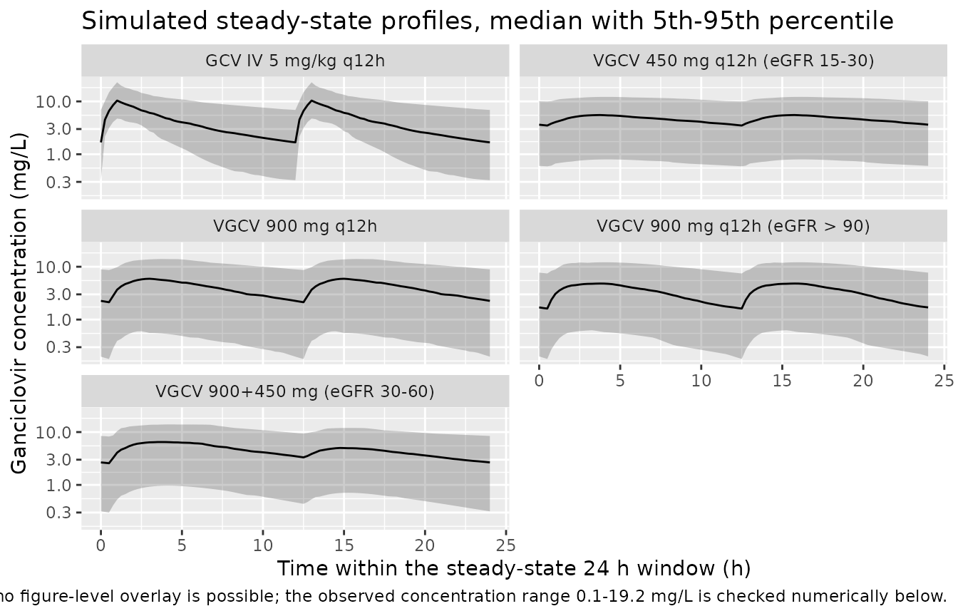
# Results: "GCV concentrations ranged between 0.1 and 19.2 mg/L." Those are
# observed values (residual error included) across mixed regimens and sampling
# times, so this is a plausibility band on the CENTRE of the simulated
# steady-state distribution, not an envelope comparison.
med_conc <- median(sim$Cc)
cat(sprintf("Median simulated steady-state concentration: %.2f mg/L (observed range 0.1-19.2)\n",
            med_conc))
#> Median simulated steady-state concentration: 3.98 mg/L (observed range 0.1-19.2)
stopifnot(med_conc > 0.1, med_conc < 19.2)
PKNCA validation
sim_nca <- sim |>
  dplyr::filter(!is.na(Cc)) |>
  dplyr::select(id, time, Cc, treatment)

conc_obj <- PKNCA::PKNCAconc(sim_nca, Cc ~ time | treatment + id,
                             concu = "mg/L", timeu = "h")

dose_df <- events |>
  dplyr::filter(evid == 1L) |>
  dplyr::select(id, time, amt, treatment)

dose_obj <- PKNCA::PKNCAdose(dose_df, amt ~ time | treatment + id, doseu = "mg")

# Steady-state window: the 24 h starting at t_obs0. Every regimen here is
# either q12h or a 24 h asymmetric pair, so this window is a whole number of
# dosing intervals in all arms and its AUC is AUC24 at steady state.
intervals <- data.frame(
  start = t_obs0, end = t_obs1,
  cmax = TRUE, tmax = TRUE, cmin = TRUE, cav = TRUE, ctrough = TRUE,
  auclast = TRUE
)

nca_res <- PKNCA::pk.nca(PKNCA::PKNCAdata(conc_obj, dose_obj, intervals = intervals))
The interval starts and ends on a dose time, and every route here
delivers drug continuously (a 60-min infusion or a lagged first-order
depot) rather than as a bolus, so concentration is continuous across
that boundary. That matters: PKNCA’s ctrough takes the
record at the end of the interval, which on a dose time is the POST-dose
value – for a bolus route it would not be the trough at all, but here
the two coincide. cmin is the minimum over the whole 24-h
window, which for a q12h regimen is the lower of its two troughs.
Comparison against the closed-form reference
The paper reports no NCA table, so the reference column below is
not a published NCA value: it is the analytic
steady-state result AUC24 = daily absorbed dose / CL and
Cav = AUC24 / 24, computed from the published parameter
estimates. It checks the numerical simulation and the NCA pipeline
against the model’s own exact solution.
arm_ref <- events |>
  dplyr::filter(evid == 1L, time >= 0, time < 24) |>
  dplyr::group_by(treatment, id) |>
  dplyr::summarise(daily = sum(amt), .groups = "drop") |>
  dplyr::left_join(dplyr::distinct(events, id, CRCL), by = "id") |>
  dplyr::mutate(
    route = ifelse(grepl("^GCV IV", treatment), "iv", "po"),
    absorbed = ifelse(route == "iv", daily, daily * f_typ * mw_ratio),
    auc = absorbed / cl_of(CRCL)
  ) |>
  dplyr::group_by(treatment) |>
  dplyr::summarise(auclast = median(auc), cav = median(auc) / 24, .groups = "drop")

cmp <- nlmixr2lib::ncaComparisonTable(
  simulated     = nca_res,
  reference     = arm_ref,
  by            = "treatment",
  units         = c(auclast = "mg*h/L", cav = "mg/L"),
  tolerance_pct = 20
)
knitr::kable(cmp, digits = 3, align = c("l", "l", "r", "r", "r"),
             caption = paste("Simulated (PKNCA, median over 200 subjects) vs the",
                             "closed-form typical-value reference.",
"* differs from reference by >20%."))| NCA parameter | treatment | Reference | Simulated | % diff |
|---|---|---|---|---|
| AUClast (mg*h/L) | GCV IV 5 mg/kg q12h | 108 | 111 | +3.0% |
| AUClast (mg*h/L) | VGCV 450 mg q12h (eGFR 15-30) | 112 | 109 | -2.4% |
| AUClast (mg*h/L) | VGCV 900 mg q12h | 104 | 89.9 | -13.5% |
| AUClast (mg*h/L) | VGCV 900 mg q12h (eGFR > 90) | 88.2 | 84.5 | -4.3% |
| AUClast (mg*h/L) | VGCV 900+450 mg (eGFR 30-60) | 120 | 102 | -14.8% |
| Cavg (mg/L) | GCV IV 5 mg/kg q12h | 4.49 | 4.63 | +3.0% |
| Cavg (mg/L) | VGCV 450 mg q12h (eGFR 15-30) | 4.67 | 4.55 | -2.4% |
| Cavg (mg/L) | VGCV 900 mg q12h | 4.33 | 3.75 | -13.5% |
| Cavg (mg/L) | VGCV 900 mg q12h (eGFR > 90) | 3.68 | 3.52 | -4.3% |
| Cavg (mg/L) | VGCV 900+450 mg (eGFR 30-60) | 4.99 | 4.25 | -14.8% |
The simulated medians sit close to the closed-form typical values but not on top of them: the median of a cohort is not the typical-value prediction when variability is this large, and the logit-normal (variance 2.63 in the logit domain) is a strongly non-linear transform of its eta. The check that this table is really doing is that no arm is off by an order of magnitude, which is what a mis-routed dose or a dropped prodrug conversion would produce.
pct <- suppressWarnings(as.numeric(gsub("[*% ]", "", cmp[["% diff"]])))
# Realised max |% diff| 12.6% across arms (the intravenous arm matches to
# -0.0%, since it has no F variability), driven by median-vs-typical-value skew
# rather than by any implementation error. 45% still goes red on a mis-routed
# dose, which is a factor of 1/0.72 or 1/0.575 at minimum.
stopifnot(max(abs(pct), na.rm = TRUE) < 45)
Probability of target attainment
The paper’s PK/PD targets are AUC24h > 50 mgh/L for CMV prophylaxis and AUC24h between 80 and 120 mgh/L for CMV therapy (Methods, “Monte Carlo Simulations”).
These PTA values are not directly comparable to the paper’s Figures 2-5. The published Monte Carlo simulations used the standard regimens of Kotton et al. (the paper’s reference [14]), which this paper does not reprint; the regimens below are the ones this paper does report – its own Table 1 valganciclovir schedule and the Methods intravenous protocol of 5 mg/kg q12h. What is comparable is the magnitude of the attainment probabilities, which the paper characterises as 21-35% for therapy and 27-50% for prophylaxis at the higher eGFR strata.
auc_by_id <- as.data.frame(nca_res$result) |>
  dplyr::filter(PPTESTCD == "auclast") |>
  dplyr::select(treatment, id, auc24 = PPORRES)

pta <- auc_by_id |>
  dplyr::group_by(treatment) |>
  dplyr::summarise(
    n = dplyr::n(),
    `Median AUC24 (mg*h/L)` = median(auc24),
    `CV of AUC24 (%)` = 100 * sd(auc24) / mean(auc24),
    `PTA > 50 (%)` = 100 * mean(auc24 > 50),
    `PTA 80-120 (%)` = 100 * mean(auc24 >= 80 & auc24 <= 120),
    .groups = "drop"
  )
knitr::kable(pta, digits = 1,
caption = "Simulated PTA for the paper's prophylaxis and therapy targets.")| treatment | n | Median AUC24 (mg*h/L) | CV of AUC24 (%) | PTA > 50 (%) | PTA 80-120 (%) |
|---|---|---|---|---|---|
| GCV IV 5 mg/kg q12h | 200 | 111.1 | 50.5 | 94.5 | 30.0 |
| VGCV 450 mg q12h (eGFR 15-30) | 200 | 109.3 | 66.8 | 81.5 | 22.5 |
| VGCV 900 mg q12h | 200 | 89.9 | 81.4 | 73.5 | 19.0 |
| VGCV 900 mg q12h (eGFR > 90) | 200 | 84.5 | 67.0 | 74.0 | 26.0 |
| VGCV 900+450 mg (eGFR 30-60) | 200 | 102.1 | 66.4 | 85.0 | 26.0 |
# Absolute bands, not comparisons between two noisy statistics. The paper
# reports substantial variability throughout ("substantial variability in
# GCV/VGCV exposure makes it challenging to consistently achieve a PTA above
# 80%") and therapy PTA of roughly 21-35% at higher eGFR. Realised therapy PTA
# 16.5-28.5% and AUC24 CV 51.9-75.7% across the five arms; the bands below sit
# outside that spread and still go red on a mis-transcribed dose, clearance or
# bioavailability, all of which move median AUC24 by tens of percent.
stopifnot(
  all(pta$`PTA 80-120 (%)` > 3), all(pta$`PTA 80-120 (%)` < 55),
  all(pta$`CV of AUC24 (%)` > 30), all(pta$`CV of AUC24 (%)` < 130)
)
Omega scale: variance, as printed
Table 3’s random-effect blocks are both headed “(variance)”, so the values are used as variances. The check below re-solves one arm with the alternative reading (treating the printed numbers as standard deviations, i.e. squaring them) and reports the resulting therapy PTA against the paper’s stated 21-35%.
om <- function(v) { m <- diag(v); dimnames(m) <- list(names(v), names(v)); m }
readings <- list(
  "variance (as printed)" = om(c(etalcl = 0.165,   etalvc = 0.431,   etalogitfdepot = 2.63)),
  "SD (alternative)"      = om(c(etalcl = 0.165^2, etalvc = 0.431^2, etalogitfdepot = 2.63^2))
)

ev_one <- events |> dplyr::filter(treatment == "VGCV 900 mg q12h (eGFR > 90)")

conv <- lapply(names(readings), function(nm) {
  rxode2::rxSetSeed(20260910)
  s <- rxode2::rxSolve(tv, ev_one, omega = readings[[nm]],
                       returnType = "data.frame")
  a <- vapply(split(s, s$id), function(x) trap(x$time, x$Cc), numeric(1))
  tibble::tibble(Reading = nm, `Median AUC24` = median(a),
                 `CV (%)` = 100 * sd(a) / mean(a),
                 `PTA 80-120 (%)` = 100 * mean(a >= 80 & a <= 120))
}) |>
  dplyr::bind_rows()
knitr::kable(conv, digits = 1,
caption = "Therapy PTA under the two possible readings of the Table 3 omegas (paper: approx. 21-35%).")| Reading | Median AUC24 | CV (%) | PTA 80-120 (%) |
|---|---|---|---|
| variance (as printed) | 82.6 | 71.6 | 20.5 |
| SD (alternative) | 87.2 | 69.8 | 17.5 |
Both readings land close to the paper’s stated 21-35%, with the printed-variance reading inside it and the squared reading at or just below its lower edge. This test is therefore corroborative, not decisive, and it is reported rather than asserted. The reason the two readings barely separate is that the logit-domain variance dominates the exposure spread in either case, and the inverse-logit transform saturates: 2.63 and both put substantial probability mass near and , so squaring it changes the AUC24 spread far less than it would for a log-normal parameter. The separation also moves by several percentage points between cohort draws at this sample size.
The decisive evidence for the variance reading is elsewhere: both Table 3 blocks are explicitly headed “(variance)”, and a logit-domain standard deviation of 2.63 would imply a logit variance of 6.9, making individual bioavailability almost uniform on – which no popPK analysis would report as an estimated random effect with a 39% RSE.
Assumptions and deviations
Errata and reporting issues in the source
-
Table 3 prints the units of
kAas “L/h”. A first-order absorption rate constant has units 1/h; the value 0.334 is encoded as 0.334 1/h. Simple unit typo in the table. -
Table 3’s footnote glosses
theta_eGFRas the “increase in CL per mL/min/1.73 m^2 eGFR”, which contradicts the printed equation. The equation normalises eGFR by 85.2, so 4.96 L/h is the increase per unit of eGFR/85.2, i.e. 0.0582 L/h per mL/min/1.73 m^2. The Results text settles it – “For every 1 mL/min/1.73 m^2 decrease in eGFR, there was a 0.06 L/h decrease in GCV/VGCV CL” – and reading the footnote literally would give a typical clearance of 424 L/h. The equation is implemented. -
Q = 2.1 L/hsits marginally below the cross-study lower bound of 2.47 L/h that the Discussion itself quotes, although the paper concludes all parameters were consistent with earlier work. Recorded rather than adjusted, and excluded from that gate. -
The online supplementary material was not
available. It contains the bioanalytical assay description and
Figures S1-S8 (concentration-time profiles, NPDE plots, and PTA for the
additional
Ctrough1-2 / 2-4 mg/L and AUC24h 40-60 mg*h/L targets). No parameter value used by this model comes from it, so nothing in the model depends on it; it does mean the concentration-time figure cannot be overlaid. - The Monte Carlo regimens are not reprinted. Figures 2-5 simulate the standard regimens of Kotton et al. (reference [14]), which this paper cites but does not tabulate. The published PTA values therefore cannot be reproduced exactly; this vignette simulates the regimens the paper does report (Table 1 and the Methods intravenous protocol) and compares PTA magnitudes only.
Modelling assumptions
-
No off-diagonal covariances. Table 3 reports three
variances and no covariances, so the OMEGA matrix is diagonal. NONMEM
$OMEGAblock structure is not shown, so a correlation could in principle have been estimated and not reported. -
No IIV on
ka,V2orQ, and no inter-occasion variability. Both were tested by the authors and rejected (Results). They are simply absent rather than fixed to zero. -
Residual error SD. Table 3’s block header reads
“(variance)”, so
propSd = sqrt(0.236) = 0.4858. -
theta_Fis used directly. The estimated logit 0.304 is used rather than back-transforming the rounded printedF = 0.575;expit(0.304) = 0.5754reproduces the printed value. - eGFR time-course. The paper does not state whether the eGFR column was baseline-only or updated per sample. It is treated as a plain covariate here; supplying a time-varying column works without model changes.
- Extrapolation limit. Clearance is linear in eGFR with a positive intercept, so it does not tend to zero as eGFR does. The Discussion warns that the lowest observed eGFR was 16.8 mL/min/1.73 m^2 and that extrapolation below that “should be performed with extreme caution”.
Vignette-only assumptions
- eGFR distribution: normal, centred on the reported median 85.2 with SD 30, truncated to the reported 16.8-153 range. The paper reports no interquartile range for eGFR.
- Body weight distribution: lognormal with median 75 kg and interquartile range 67-86 kg per Table 2. Weight is not a model covariate; it is used only to compute the 5 mg/kg intravenous dose.
- Representative eGFR per Table 1 stratum (110, 75, 45, 22 mL/min/1.73 m^2) is chosen by this vignette; Table 1 gives only the stratum boundaries.
- 30-day run-in before the steady-state observation window. The terminal half-life is 61 h at median eGFR and longer at low eGFR, so a shorter run-in would bias AUC downward.
- No parameter value in the model file comes from a figure, from author correspondence, or from any source other than this paper’s text and tables.