Cefazolin (Bindellini 2025)
Source:vignettes/articles/Bindellini_2025_cefazolin.Rmd
Bindellini_2025_cefazolin.RmdModel and source
- Citation: Bindellini D, Simon P, Busse D, Michelet R, Petroff D, Aulin LBS, Dorn C, Zeitlinger M, Huisinga W, Wrigge H, Kloft C. Evaluation of the need for dosing adaptations in obese patients for surgical antibiotic prophylaxis: a model-based analysis of cefazolin pharmacokinetics. Br J Anaesth. 2025;134(4):1041-1049. doi:10.1016/j.bja.2024.11.044. PMCID PMC11947583. Parameter estimates from Table 2; model structure from Figure 1 and the Results text; the authors’ deposited mrgsolve simulation code (github.com/Kloft-Lab/Bindellini-et-al._CefazolinPK_Obese_Nonobese_mrgsolve_model, popPK_CEZ_run077.cpp, cited in the Supplementary Material) confirms the LBW/FM scaling, the binding equation and Cisf = TF * C2.
- Description: Two-compartment population PK model for intravenous cefazolin in obese (bariatric surgery, BMI >= 35 kg/m^2) and nonobese surgical adults with plasma and subcutaneous adipose-tissue microdialysis data (Bindellini 2025). The model is parameterised on UNBOUND cefazolin: Cu = central/V1 with linear unbound clearance, and the measured total plasma concentration is Cc = Cu + Bmax * Cu / (Kd + Cu) (saturable protein binding). V1 scales linearly and Q to the 0.75 power with lean body weight (fat-free mass, Janmahasatian); V2 follows the LBW/FM approach, with a fraction R scaling with lean body weight and the rest with fat mass. The interstitial-fluid concentration is a tissue factor times the peripheral-compartment concentration, Cisf = TF * C2; microdialysate concentrations are Cisf times the catheter relative recovery RR, which differs between obese and nonobese patients and carries inter-individual and inter-catheter variability, and retrodialysis observes 1 - RR.
- Article (open access): https://doi.org/10.1016/j.bja.2024.11.044
- Authors’ mrgsolve simulation code: https://github.com/Kloft-Lab/Bindellini-et-al._CefazolinPK_Obese_Nonobese_mrgsolve_model
mod <- readModelDb("Bindellini_2025_cefazolin")
ui <- rxode2::rxode(mod)
#> ℹ parameter labels from comments will be replaced by 'label()'
Population
Bindellini 2025 is a post hoc model-based analysis of a prospective, controlled, single-centre, open-label trial at Leipzig University (EudraCT 2012-004383-22). Fifteen obese patients (BMI >= 35 kg/m^2; median 52.6, range 39.5-69.3) undergoing bariatric surgery and 15 age- and sex-matched nonobese patients (median BMI 26.0, range 18.7-29.8) undergoing elective abdominal surgery each received a single 2 g cefazolin dose as a 30-minute intravenous infusion after induction of general anaesthesia (Methods; Table 1). Two thirds of each group were women; the median age was 45 years (range 21-65). Lean body weight (Janmahasatian) had a median of 64.3 kg (range 34.2-96.1) and fat mass a median of 41.5 kg (range 15.8-122); these two medians are the reference values of the body-size scaling.
Total cefazolin was measured in plasma at 0.5, 1, 2, 3, 4, 5, 6 and 8 h and unbound cefazolin (ultrafiltration) at 0.5, 1, 4 and 8 h. Two microdialysis catheters per patient, one in the subcutaneous adipose tissue of each upper arm, collected dialysate over ten intervals from 0-0.5 h to 7-8 h, and three 15-minute retrodialysis samples per patient followed the sampling period to calibrate the catheter relative recovery.
The same information is available programmatically via
readModelDb("Bindellini_2025_cefazolin")()$population.
Model structure
The model is a two-compartment model written in terms of unbound cefazolin (Methods: “The model was parameterised in terms of cefazolin unbound concentrations”):
-
Cu = central / V1, with linear unbound clearance CL (17.9 L/h, no covariate). - Total plasma concentration through saturable binding,
Cc = Cu + Bmax * Cu / (Kd + Cu), Bmax 247 mg/L and Kd 65.3 mg/L. At low concentrations the unbound fraction tends toKd / (Kd + Bmax)= 20.9%. - Body size (Results): V1 scales linearly and Q with exponent 0.75 on
lean body weight (
FFM, reference 64.3 kg); V2 follows the LBW/FM approach,V2 = 34.3 * (0.764 * FFM / 64.3 + 0.236 * FM / 41.5). - The adipose interstitial-fluid concentration is a tissue factor
times the peripheral-compartment concentration,
Cisf = 0.655 * C2. - Microdialysis: the dialysate concentration is
Cmd = RR * Cisf, with the catheter relative recovery RR = 41.1% in nonobese and 23.3% in obese patients (DIS_OBESE), log-normal inter-individual variability and an additional intercatheter random effect per catheter (MD_CATHETER). Retrodialysis observesCrd_ratio = C_RD / C_RP = 1 - RR.
Obesity acts only on RR, a property of the microdialysis technique in the tissue; it changes no drug parameter. Drug exposure differs between obese and nonobese patients only through lean body weight and fat mass.
Source trace
| Element | Value | Source |
|---|---|---|
| Two-compartment structure, linear elimination | – | Results, ‘Pharmacokinetic model’; Figure 1 |
| Parameterisation on unbound concentration | – | Methods, ‘Pharmacokinetic model development’ |
lcl |
log(17.9) L/h | Table 2, CL |
lvc |
log(22.9) L at LBW 64.3 kg | Table 2, V1 |
e_ffm_vc |
1 (fixed) | Table 2, Exponent V1 |
lq |
log(56.8) L/h at LBW 64.3 kg | Table 2, Q |
e_ffm_q |
0.75 (fixed) | Table 2, Exponent Q |
lvp |
log(34.3) L at LBW 64.3 kg, FM 41.5 kg | Table 2, V2 |
f_ffm_vp |
0.764 | Table 2, R; Results (‘23.6% … depend on FM’) |
| LBW/FM equation for V2 | – | Table 2 footnote; authors’ mrgsolve code
V2=TVV2*((LBW/64.3)*R+(FM/41.5)*(1-R))
|
lbmax_pb |
log(247) mg/L | Table 2, Bmax; Results |
lkd_pb |
log(65.3) mg/L | Table 2, Kd; Results |
Binding equation Cc = Cu + Bmax*Cu/(Kd+Cu)
|
– | Results; Supplementary Fig. S1; mrgsolve code
CT=CU+(CU*BMAX/(CU+KD))
|
ratio_isf_peripheral1 |
0.655 | Table 2, TF; Results |
Cisf = TF * C2 |
– | Results; Figure 1; mrgsolve code CISF=(P/V2)*TF
|
lrr_md |
log(0.411) | Table 2, RRnonobese |
lrr_md_obese |
log(0.233) | Table 2, RRobese |
Cmd = RR * Cisf; Crd_ratio = 1 - RR
|
– | Results; Figure 1; Methods (retrodialysis calibration) |
etalcl, etalvc, etalq,
etalvp, etalbmax_pb
|
21.9, 40.1, 54.8, 12.4, 9.20% CV | Table 2, interindividual variability |
etalrr_md |
43.3% CV | Table 2, RR |
etaiov_lrr_md (per catheter) |
58.6% CV | Table 2, Intercatheter |
propSd, propSd_Cu
|
0.357 | Table 2, plasma proportional error (total and unbound) |
propSd_Cmd |
0.521 | Table 2, microdialysis proportional error |
propSd_Crd_ratio |
0.289 | Table 2, retrodialysis proportional error |
The CV% values are converted to log-scale variances with
omega^2 = log(CV^2 + 1).
Reference patients
The paper’s dosing evaluation (Methods) uses three reference patients
given by total body weight and percent fat mass. Fat mass is
WT * FM% and lean body weight the remainder.
ref_pts <- tibble(
  patient = factor(
    c("Nonobese", "Obese", "Morbidly obese"),
    levels = c("Nonobese", "Obese", "Morbidly obese")
  ),
  WT = c(70, 95.1, 127),
  fm_pct = c(24.8, 29.5, 39.5),
  BMI = c(24.2, 33.0, 44.0)
) |>
  mutate(FM = WT * fm_pct / 100, FFM = WT - FM)

ref_pts |>
  dplyr::rename(
    "Reference patient" = patient,
    "TBW (kg)" = WT,
    "FM (%)" = fm_pct,
    "BMI (kg/m^2)" = BMI,
    "FM (kg)" = FM,
    "LBW (kg)" = FFM
  ) |>
knitr::kable(digits = 1)| Reference patient | TBW (kg) | FM (%) | BMI (kg/m^2) | FM (kg) | LBW (kg) |
|---|---|---|---|---|---|
| Nonobese | 70.0 | 24.8 | 24.2 | 17.4 | 52.6 |
| Obese | 95.1 | 29.5 | 33.0 | 28.1 | 67.0 |
| Morbidly obese | 127.0 | 39.5 | 44.0 | 50.2 | 76.8 |
Dosing-regimen simulation (Figures 2 and 3)
Four regimens, each a 30-minute infusion with the same dose repeated at 3 or 4 h, are simulated for 200 virtual patients per reference patient and regimen with inter-individual variability (the paper used 1000).
regimens <- tibble(
  regimen = factor(
    c("1 g (redosing 3 h)", "1 g (redosing 4 h)", "2 g (redosing 3 h)", "2 g (redosing 4 h)"),
    levels = c("1 g (redosing 3 h)", "1 g (redosing 4 h)", "2 g (redosing 3 h)", "2 g (redosing 4 h)")
  ),
  dose = c(1000, 1000, 2000, 2000),
  redose = c(3, 4, 3, 4)
)

n_per_arm <- 200
obs_times <- seq(0, 8, by = 0.05)

arms <- tidyr::crossing(ref_pts, regimens) |>
  mutate(arm = row_number())

subjects <- arms |>
  tidyr::uncount(n_per_arm) |>
  mutate(id = row_number())

dose_rows <- subjects |>
  rowwise() |>
  reframe(
    id = id,
    time = seq(0, 7.99, by = redose),
    amt = dose,
    rate = dose / 0.5
  ) |>
  mutate(evid = 1L, cmt = "central", dvid = NA_integer_)

obs_rows <- subjects |>
  select(id) |>
  tidyr::crossing(time = obs_times) |>
  mutate(amt = 0, rate = 0, evid = 0L, cmt = "central", dvid = 1L)

ev_reg <- bind_rows(dose_rows, obs_rows) |>
  left_join(
    subjects |> select(id, patient, regimen, FFM, FM),
    by = "id"
  ) |>
  mutate(DIS_OBESE = 0L, MD_CATHETER = 1L) |>
  arrange(id, time, desc(evid))

# The intercatheter random effect needs at least two catheter levels in the
# data to be simulated; one extra subject carries catheter 2 and is dropped.
ev_reg <- bind_rows(
  ev_reg,
  ev_reg |> filter(id == 1) |> mutate(id = max(ev_reg$id) + 1L, MD_CATHETER = 2L)
)

rxode2::rxSetSeed(20250401)
sim_reg <- rxode2::rxSolve(
  mod,
  events = ev_reg,
  keep = c("patient", "regimen"),
  returnType = "data.frame"
) |>
  filter(id <= nrow(subjects))
#> ℹ parameter labels from comments will be replaced by 'label()'
Figure 2: unbound plasma and ISF concentrations
fig2 <- sim_reg |>
  select(id, time, patient, regimen, Plasma = Cu, ISF = Cisf) |>
  tidyr::pivot_longer(c(Plasma, ISF), names_to = "matrix", values_to = "conc") |>
  mutate(matrix = factor(matrix, levels = c("Plasma", "ISF"))) |>
  group_by(patient, regimen, matrix, time) |>
  summarise(
    p05 = quantile(conc, 0.05),
    p50 = median(conc),
    p95 = quantile(conc, 0.95),
    .groups = "drop"
  )

ggplot(fig2, aes(time, p50, colour = patient, fill = patient)) +
  geom_ribbon(aes(ymin = p05, ymax = p95), alpha = 0.15, colour = NA) +
  geom_line(linewidth = 0.8) +
  geom_hline(yintercept = 4, linetype = "dashed") +
  facet_grid(regimen ~ matrix, scales = "free_y") +
  labs(
    x = "Time (h)", y = "Unbound cefazolin (mg/L)", colour = NULL, fill = NULL,
    caption = "Replicates Figure 2 of Bindellini 2025: median and 5th-95th percentiles; dashed line MIC 4 mg/L."
  ) +
  theme_bw() +
  theme(legend.position = "bottom")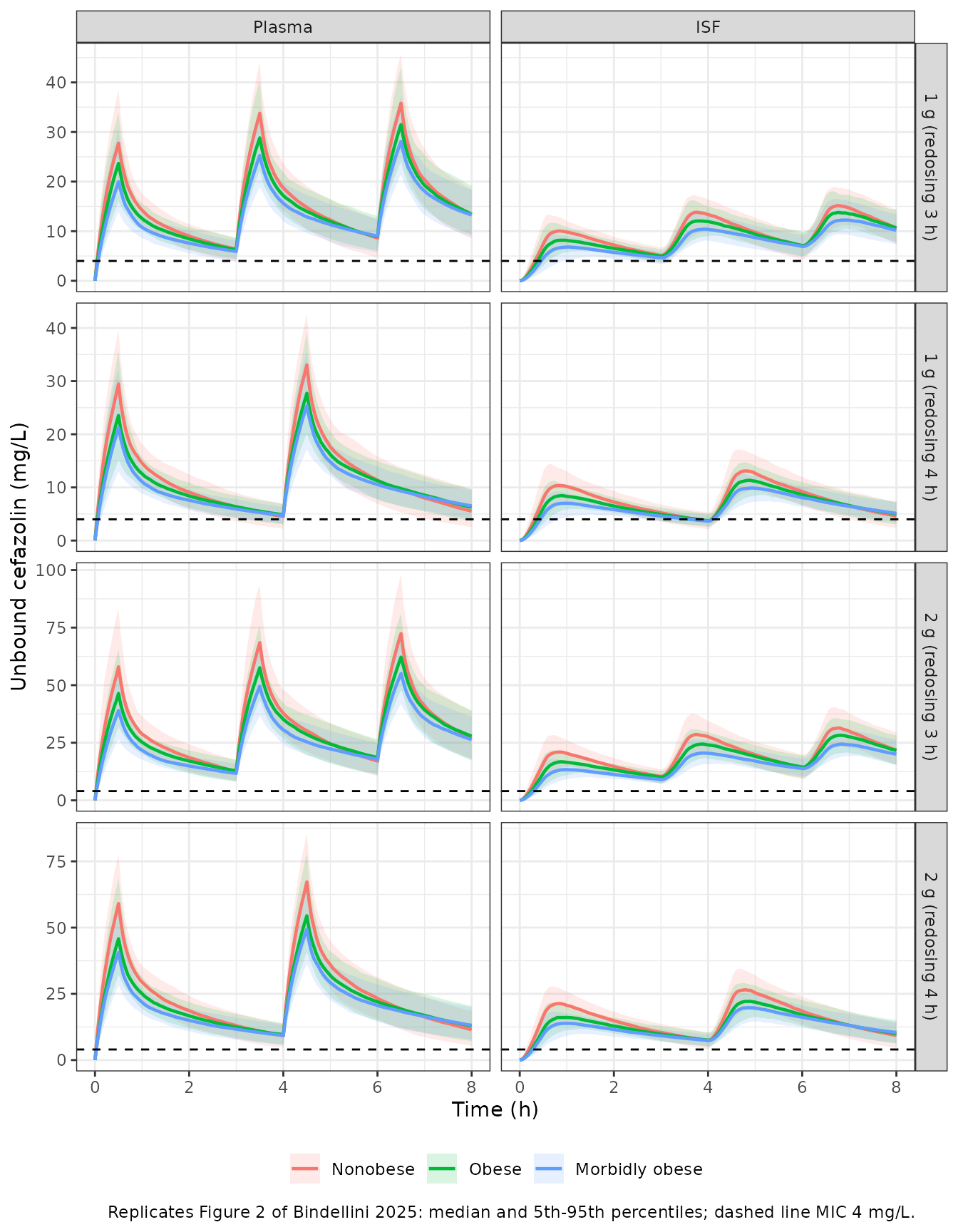
The medians read off Figure 2 of the paper give a check of the typical exposure in each reference patient: the first unbound plasma peak after 1 g is about 27 mg/L (nonobese) and 20 mg/L (morbidly obese), and the first ISF peak after 2 g about 20.5 mg/L (nonobese) and 13.5 mg/L (morbidly obese).
fig2_ref <- tibble(
  patient = c("Nonobese", "Morbidly obese", "Nonobese", "Morbidly obese"),
  regimen = c("1 g (redosing 4 h)", "1 g (redosing 4 h)", "2 g (redosing 4 h)", "2 g (redosing 4 h)"),
  matrix = c("Plasma", "Plasma", "ISF", "ISF"),
  published = c(27, 20, 20.5, 13.5)
)

fig2_sim <- fig2 |>
  filter(time <= 2) |>
  group_by(patient, regimen, matrix) |>
  summarise(simulated = max(p50), .groups = "drop") |>
  mutate(across(c(patient, regimen, matrix), as.character))

fig2_cmp <- fig2_ref |>
  left_join(fig2_sim, by = c("patient", "regimen", "matrix")) |>
  mutate(pct_diff = 100 * (simulated - published) / published)

fig2_cmp |>
  dplyr::rename(
    "Reference patient" = patient, Regimen = regimen, Matrix = matrix,
    "Figure 2 median peak (mg/L)" = published,
    "Simulated median peak (mg/L)" = simulated,
    "Difference (%)" = pct_diff
  ) |>
knitr::kable(digits = 1)| Reference patient | Regimen | Matrix | Figure 2 median peak (mg/L) | Simulated median peak (mg/L) | Difference (%) |
|---|---|---|---|---|---|
| Nonobese | 1 g (redosing 4 h) | Plasma | 27.0 | 29.5 | 9.2 |
| Morbidly obese | 1 g (redosing 4 h) | Plasma | 20.0 | 21.2 | 6.0 |
| Nonobese | 2 g (redosing 4 h) | ISF | 20.5 | 21.4 | 4.3 |
| Morbidly obese | 2 g (redosing 4 h) | ISF | 13.5 | 13.9 | 2.7 |
Figure 3: probability of target attainment
The target is unbound cefazolin above the MIC for 100% of the 8-hour evaluation period (fT>MIC = 100%). Concentrations are zero at the start of the first infusion, so the period is taken from the end of the first infusion (0.5 h) to 8 h; this reading reproduces the PTA values the paper reports in the text (next chunk).
mics <- c(0.25, 0.5, 1, 2, 4)

min_conc <- sim_reg |>
  filter(time >= 0.5) |>
  group_by(patient, regimen, id) |>
  summarise(Plasma = min(Cu), ISF = min(Cisf), .groups = "drop") |>
  tidyr::pivot_longer(c(Plasma, ISF), names_to = "matrix", values_to = "cmin")

pta <- tidyr::crossing(min_conc, MIC = mics) |>
  group_by(patient, regimen, matrix, MIC) |>
  summarise(PTA = 100 * mean(cmin >= MIC), .groups = "drop") |>
  mutate(matrix = factor(matrix, levels = c("Plasma", "ISF")))

ggplot(pta, aes(factor(MIC), PTA, colour = patient, group = patient)) +
  annotate("rect", xmin = -Inf, xmax = Inf, ymin = 90, ymax = 100, fill = "palegreen", alpha = 0.5) +
  geom_line() +
  geom_point() +
  facet_grid(matrix ~ regimen) +
  labs(
    x = "MIC (mg/L)", y = "PTA (%)", colour = NULL,
    caption = "Replicates the PTA curves of Figure 3 of Bindellini 2025 (MIC distributions not shown)."
  ) +
  theme_bw() +
  theme(legend.position = "bottom")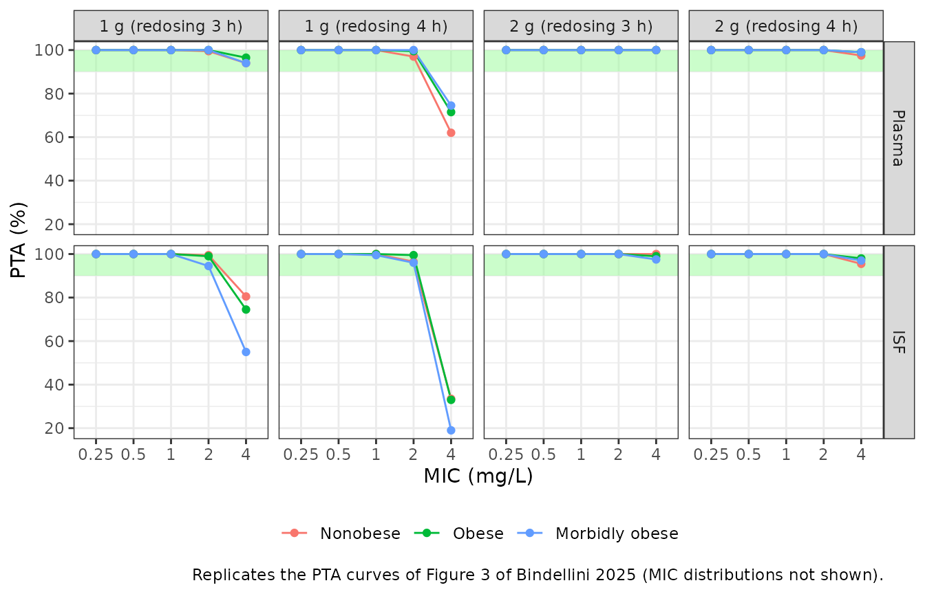
The Results text reports six PTA values at MIC 4 mg/L: unbound plasma after 1 g with redosing at 4 h, and ISF after 1 g with redosing at 3 h.
pta_ref <- tibble(
  matrix = rep(c("Plasma", "ISF"), each = 3),
  regimen = rep(c("1 g (redosing 4 h)", "1 g (redosing 3 h)"), each = 3),
  patient = rep(c("Nonobese", "Obese", "Morbidly obese"), 2),
  published = c(60.9, 73.4, 74.5, 85.5, 75.1, 61.2)
)

pta_cmp <- pta_ref |>
  left_join(
    pta |>
      filter(MIC == 4) |>
      mutate(across(c(patient, regimen, matrix), as.character)),
    by = c("matrix", "regimen", "patient")
  ) |>
  mutate(diff_pp = PTA - published)

pta_cmp |>
  select(matrix, regimen, patient, published, PTA, diff_pp) |>
  dplyr::rename(
    Matrix = matrix, Regimen = regimen, "Reference patient" = patient,
    "Published PTA (%)" = published, "Simulated PTA (%)" = PTA,
    "Difference (percentage points)" = diff_pp
  ) |>
knitr::kable(digits = 1)| Matrix | Regimen | Reference patient | Published PTA (%) | Simulated PTA (%) | Difference (percentage points) |
|---|---|---|---|---|---|
| Plasma | 1 g (redosing 4 h) | Nonobese | 60.9 | 62.0 | 1.1 |
| Plasma | 1 g (redosing 4 h) | Obese | 73.4 | 71.5 | -1.9 |
| Plasma | 1 g (redosing 4 h) | Morbidly obese | 74.5 | 74.5 | 0.0 |
| ISF | 1 g (redosing 3 h) | Nonobese | 85.5 | 80.5 | -5.0 |
| ISF | 1 g (redosing 3 h) | Obese | 75.1 | 74.5 | -0.6 |
| ISF | 1 g (redosing 3 h) | Morbidly obese | 61.2 | 55.0 | -6.2 |
# 200 patients per arm give a Monte Carlo standard error of about 3.5
# percentage points at these PTAs, so the gate is on the mean absolute
# difference, with a looser envelope for any one value.
stopifnot(
  mean(abs(pta_cmp$diff_pp)) < 7,
  all(abs(pta_cmp$diff_pp) < 15)
)
The paper’s conclusions are reproduced: at MIC <= 2 mg/L every regimen reaches PTA >= 90% in plasma and ISF for all three reference patients, while at MIC 4 mg/L 1 g with redosing at 4 h fails in plasma and 1 g with redosing at 3 h fails in ISF, and obesity changes PTA only modestly.
Closed-form checks on the typical patient
For the typical patient (no random effects) the unbound AUC from zero
to infinity of a single 2 g dose is Dose / CL = 111.7
mg*h/L whatever the body size, and the unbound fraction at low
concentrations is Kd / (Kd + Bmax).
mod_typ <- rxode2::zeroRe(mod)
#> ℹ parameter labels from comments will be replaced by 'label()'

ev_typ <- ref_pts |>
  filter(patient %in% c("Nonobese", "Morbidly obese")) |>
  mutate(id = row_number()) |>
  select(id, patient, FFM, FM) |>
  rowwise() |>
  reframe(
    id = id, patient = patient, FFM = FFM, FM = FM,
    time = c(0, seq(0, 48, by = 0.05)),
    amt = c(2000, rep(0, length(seq(0, 48, by = 0.05)))),
    rate = c(4000, rep(0, length(seq(0, 48, by = 0.05)))),
    evid = c(1L, rep(0L, length(seq(0, 48, by = 0.05)))),
    dvid = c(NA_integer_, rep(1L, length(seq(0, 48, by = 0.05))))
  ) |>
  # rxode2 needs at least two levels of the catheter nesting column in the
  # data even when the random effects are zeroed.
  mutate(cmt = "central", DIS_OBESE = 0L, MD_CATHETER = id)

sim_typ <- rxode2::rxSolve(
  mod_typ,
  events = ev_typ,
  keep = "patient",
  returnType = "data.frame",
  atol = 1e-10, rtol = 1e-10
)

fu_low <- with(tail(sim_typ, 1), Cu / Cc)
fu_expected <- 65.3 / (65.3 + 247)
stopifnot(abs(fu_low - fu_expected) / fu_expected < 1e-3)
NCA with PKNCA
Noncompartmental analysis of the single 2 g dose for the two typical patients, on unbound and total plasma concentration.
nca_conc <- sim_typ |>
  filter(!is.na(Cu)) |>
  select(id, time, patient, Cu, Cc) |>
  tidyr::pivot_longer(c(Cu, Cc), names_to = "analyte", values_to = "conc") |>
  mutate(treatment = paste(patient, analyte)) |>
  distinct(id, treatment, time, .keep_all = TRUE)

nca_dose <- ev_typ |>
  filter(evid == 1) |>
  select(id, time, amt, patient) |>
  tidyr::crossing(analyte = c("Cu", "Cc")) |>
  mutate(treatment = paste(patient, analyte))

conc_obj <- PKNCA::PKNCAconc(nca_conc, conc ~ time | treatment + id)
dose_obj <- PKNCA::PKNCAdose(nca_dose, amt ~ time | treatment + id, route = "intravascular", duration = 0.5)
intervals <- data.frame(
  start = 0, end = Inf,
  cmax = TRUE, tmax = TRUE, aucinf.obs = TRUE, half.life = TRUE
)
nca_res <- PKNCA::pk.nca(PKNCA::PKNCAdata(conc_obj, dose_obj, intervals = intervals))

nca_tbl <- as.data.frame(nca_res) |>
  filter(PPTESTCD %in% c("cmax", "tmax", "aucinf.obs", "half.life")) |>
  select(treatment, PPTESTCD, PPORRES) |>
  tidyr::pivot_wider(names_from = PPTESTCD, values_from = PPORRES)

nca_tbl |>
  dplyr::rename(
    "Patient and analyte" = treatment,
    "Cmax (mg/L)" = cmax,
    "Tmax (h)" = tmax,
    "AUC0-inf (mg*h/L)" = aucinf.obs,
    "t1/2 (h)" = half.life
  ) |>
knitr::kable(digits = 2)| Patient and analyte | Cmax (mg/L) | Tmax (h) | t1/2 (h) | AUC0-inf (mg*h/L) |
|---|---|---|---|---|
| Morbidly obese Cc | 139.74 | 0.5 | 2.96 | 460.93 |
| Morbidly obese Cu | 42.44 | 0.5 | 2.93 | 111.72 |
| Nonobese Cc | 174.20 | 0.5 | 1.92 | 434.44 |
| Nonobese Cu | 58.01 | 0.5 | 1.90 | 111.72 |
auc_u <- nca_tbl$aucinf.obs[grepl(" Cu$", nca_tbl$treatment)]
stopifnot(all(abs(auc_u - 2000 / 17.9) / (2000 / 17.9) < 0.01))

# Terminal half-life of the two-compartment unbound disposition, from the
# micro-constants of each typical patient.
hl_check <- sim_typ |>
  filter(!is.na(Cu)) |>
  group_by(patient) |>
  slice(1) |>
  ungroup() |>
  mutate(
    beta = 0.5 * ((kel + k12 + k21) - sqrt((kel + k12 + k21)^2 - 4 * kel * k21)),
    t_half_closed = log(2) / beta,
    treatment = paste(patient, "Cu")
  ) |>
  select(treatment, t_half_closed) |>
  left_join(nca_tbl |> select(treatment, half.life), by = "treatment")
hl_check
#> # A tibble: 2 × 3
#>   treatment         t_half_closed half.life
#>   <chr>                     <dbl>     <dbl>
#> 1 Nonobese Cu                1.91      1.90
#> 2 Morbidly obese Cu          2.93      2.93
stopifnot(all(abs(hl_check$half.life / hl_check$t_half_closed - 1) < 0.02))
The unbound AUC equals Dose / CL (111.7 mg*h/L) in both
typical patients: clearance carries no body-size term, and the greater
lean body weight and fat mass of the morbidly obese patient only lowers
the early peak and prolongs the terminal phase. The terminal half-life
of the nonobese reference patient (about 1.9 h) is in the 1.5-2 h range
the paper’s Discussion quotes for cefazolin; in the morbidly obese
reference patient the larger V1 and V2 at the same clearance lengthen it
to about 3 h. Bindellini 2025 itself reports no NCA parameters (the
earlier noncompartmental analysis of these data is Dorn et al. 2021), so
there is no published table to compare against.
Microdialysis measurement layer
To exercise the microdialysis and retrodialysis outputs, the trial design is simulated with 200 obese and 200 nonobese patients, each with two catheters. Lean body weight and fat mass are drawn log-normally around the cohort medians of Table 1 and truncated to the observed ranges. Microdialysate records sit at the midpoint of each collection interval; three retrodialysis records follow the 8-hour sampling period.
n_md <- 200
set.seed(2025)
md_subj <- tibble(
  id = seq_len(2 * n_md),
  DIS_OBESE = rep(c(0L, 1L), each = n_md),
  cohort = ifelse(DIS_OBESE == 1L, "Obese", "Nonobese")
) |>
  mutate(
    FFM = ifelse(DIS_OBESE == 1L, 69.3, 45.6) * exp(rnorm(n(), 0, 0.15)),
    FFM = ifelse(DIS_OBESE == 1L, pmin(pmax(FFM, 54.9), 96.1), pmin(pmax(FFM, 34.2), 72.4)),
    FM = ifelse(DIS_OBESE == 1L, 84.2, 25.0) * exp(rnorm(n(), 0, 0.2)),
    FM = ifelse(DIS_OBESE == 1L, pmin(pmax(FM, 48.8), 122), pmin(pmax(FM, 15.8), 34.2))
  )

md_start <- c(0, 0.5, 1, 1.5, 2, 3, 4, 5, 6, 7)
md_end <- c(0.5, 1, 1.5, 2, 3, 4, 5, 6, 7, 8)
md_mid <- (md_start + md_end) / 2

# dvid follows the order of the residual-error lines in model():
# 1 Cc, 2 Cu, 3 Cmd, 4 Crd_ratio.
plasma_obs <- tidyr::crossing(id = md_subj$id, time = c(0.5, 1, 2, 3, 4, 5, 6, 8)) |>
  mutate(dvid = 1L, MD_CATHETER = 1L)
unbound_obs <- tidyr::crossing(id = md_subj$id, time = c(0.5, 1, 4, 8)) |>
  mutate(dvid = 2L, MD_CATHETER = 1L)
md_obs <- tidyr::crossing(id = md_subj$id, time = md_mid, MD_CATHETER = 1:2) |>
  mutate(dvid = 3L)
rd_obs <- tidyr::crossing(id = md_subj$id, time = c(8.125, 8.375, 8.625), MD_CATHETER = 1:2) |>
  mutate(dvid = 4L)

ev_md <- bind_rows(
  tibble(id = md_subj$id, time = 0, amt = 2000, rate = 4000, evid = 1L, dvid = NA_integer_, MD_CATHETER = 1L),
  bind_rows(plasma_obs, unbound_obs, md_obs, rd_obs) |> mutate(amt = 0, rate = 0, evid = 0L)
) |>
  mutate(
    cmt = "central",
    endpoint = c("Cc", "Cu", "Cmd", "Crd_ratio")[dvid],
    catheter = MD_CATHETER
  ) |>
  left_join(md_subj, by = "id") |>
  arrange(id, time, desc(evid), dvid, MD_CATHETER)

rxode2::rxSetSeed(2026)
sim_md <- rxode2::rxSolve(
  mod,
  events = ev_md,
  keep = c("cohort", "catheter", "endpoint"),
  returnType = "data.frame"
)
sim_md |>
  filter(endpoint == "Cmd") |>
  group_by(cohort, time) |>
  summarise(
    across(c(Cisf, sim), list(p50 = median, p05 = ~ quantile(.x, 0.05), p95 = ~ quantile(.x, 0.95))),
    .groups = "drop"
  ) |>
  ggplot(aes(time)) +
  geom_ribbon(aes(ymin = sim_p05, ymax = sim_p95, fill = "Microdialysate (with residual error)"), alpha = 0.25) +
  geom_line(aes(y = sim_p50, colour = "Microdialysate (with residual error)")) +
  geom_line(aes(y = Cisf_p50, colour = "ISF (recovery-corrected)"), linewidth = 0.8) +
  facet_wrap(~cohort) +
  labs(
    x = "Time (h)", y = "Cefazolin (mg/L)", colour = NULL, fill = NULL,
    caption = "Simulated microdialysate concentrations at the collection-interval midpoints: median and 5th-95th percentiles."
  ) +
  theme_bw() +
  theme(legend.position = "bottom")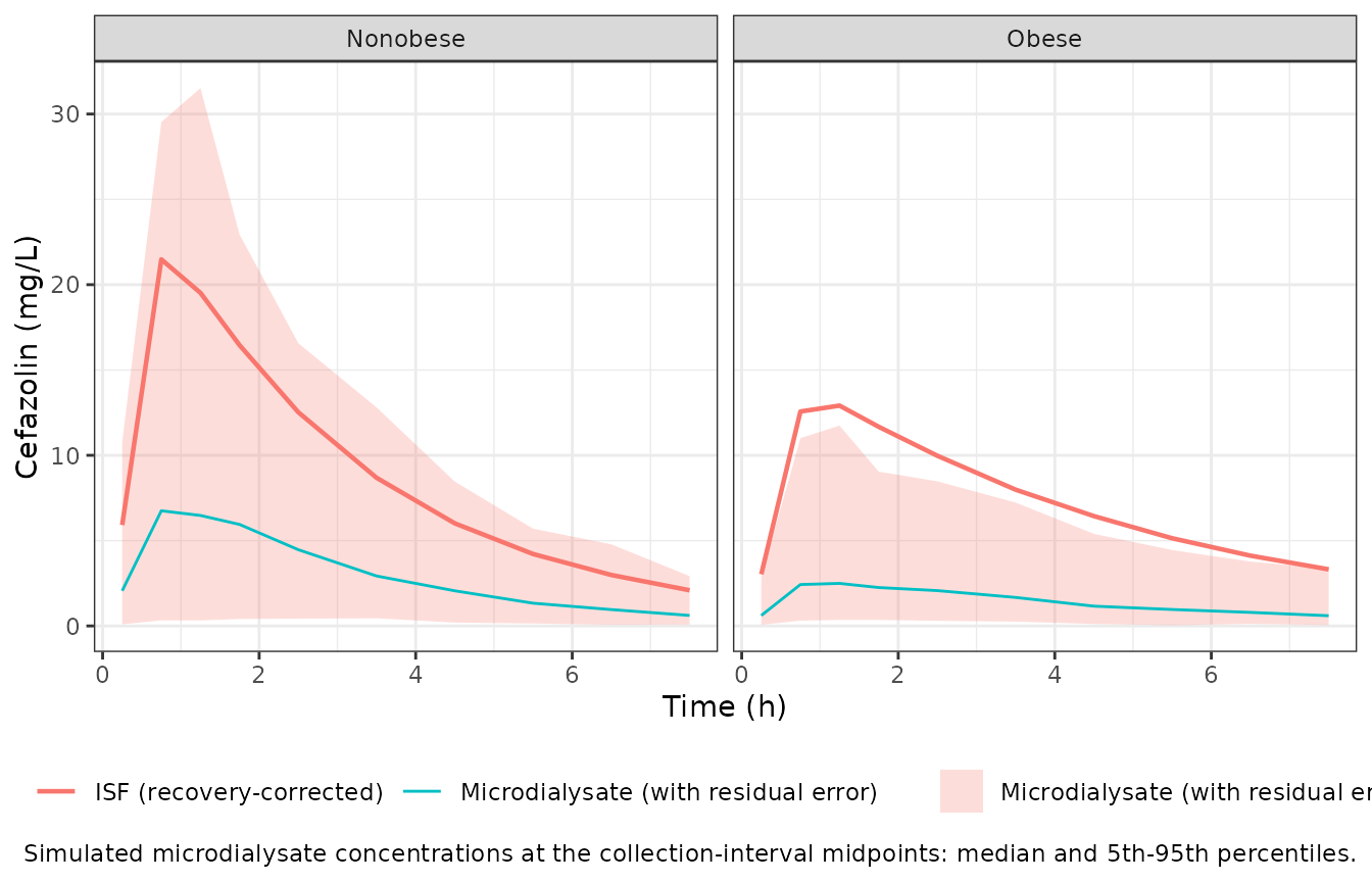
The recovery layer is checked directly: the median ratio of
microdialysate to ISF concentration is the typical RR of each cohort,
the median retrodialysis ratio is 1 - RR, and the two
catheters of a patient share the inter-individual part of the random
effect, so the correlation of their log-recoveries is
omega^2_RR / (omega^2_RR + omega^2_catheter) = 0.37.
rr_by_catheter <- sim_md |>
  filter(endpoint == "Cmd") |>
  distinct(id, cohort, catheter, rr_md)

md_tbl <- rr_by_catheter |>
  group_by(cohort) |>
  summarise(median_rr = median(rr_md), pct_rr_above_1 = 100 * mean(rr_md > 1), .groups = "drop") |>
  left_join(
    sim_md |>
      filter(endpoint == "Crd_ratio") |>
      group_by(cohort) |>
      summarise(median_crd_ratio = median(Crd_ratio), .groups = "drop"),
    by = "cohort"
  ) |>
  mutate(typical_rr = ifelse(cohort == "Obese", 0.233, 0.411))

md_tbl |>
  select(cohort, typical_rr, median_rr, median_crd_ratio, pct_rr_above_1) |>
  dplyr::rename(
    Cohort = cohort,
    "Table 2 RR" = typical_rr,
    "Median simulated RR" = median_rr,
    "Median C_RD / C_RP" = median_crd_ratio,
    "Catheters with RR > 1 (%)" = pct_rr_above_1
  ) |>
knitr::kable(digits = 3)| Cohort | Table 2 RR | Median simulated RR | Median C_RD / C_RP | Catheters with RR > 1 (%) |
|---|---|---|---|---|
| Nonobese | 0.411 | 0.381 | 0.619 | 6.5 |
| Obese | 0.233 | 0.215 | 0.785 | 1.5 |
# Centre each catheter's log-recovery on its cohort's typical value so the
# obese / nonobese difference in RR does not add to the shared variance.
cat_wide <- rr_by_catheter |>
  mutate(rr_md = rr_md / ifelse(cohort == "Obese", 0.233, 0.411)) |>
  tidyr::pivot_wider(id_cols = id, names_from = catheter, values_from = rr_md, names_prefix = "cath")
r_catheter <- cor(log(cat_wide$cath1), log(cat_wide$cath2))
r_expected <- 0.17184 / (0.17184 + 0.2952)
r_catheter
#> [1] 0.4335949

stopifnot(
  all(abs(md_tbl$median_rr / md_tbl$typical_rr - 1) < 0.2),
  all(abs(md_tbl$median_crd_ratio - (1 - md_tbl$typical_rr)) < 0.1),
  abs(r_catheter - r_expected) < 0.2
)
Assumptions and deviations
-
Random-effect scale. Table 2 reports all random
effects as CV%; they are taken as log-normal and converted with
omega^2 = log(CV^2 + 1). For RR this log-normal reading lets a catheter’s recovery exceed 1 in a minority of draws (about 10% of nonobese and 2% of obese catheters, from the 0.411 and 0.233 typical values and the combined IIV and intercatheter variance; see the table above), which would make the retrodialysis ratio1 - RRnegative. The paper does not state the RR transform; a logit-scale implementation would avoid the boundary, but there is no published value to build it from. -
Integrated dialysate. The paper analysed
microdialysis with the integrated dialysate-based approach (Tunblad et
al. 2004; Busse et al. 2021), where a dialysate value is RR times the
mean ISF concentration over its collection interval. The model evaluates
Cmd = RR * Cisfat the record time, so dialysate records belong at the collection-interval midpoint; for the 0-0.5 h and 0.5-1 h intervals, where the ISF concentration is rising steeply, the midpoint value differs from the interval mean. - Intracatheter variability (90.3% CV in Table 2) is not encoded. It is a within-catheter random effect on RR below the level of the catheter, and rxode2 has no third nesting level for it here; leaving it out narrows the spread of simulated dialysate values but changes no drug exposure.
-
Retrodialysis.
Crd_ratio = C_RD / C_RP = 1 - RRis the calibration relation of retrodialysis by drug; it neglects any cefazolin still in the ISF during the retrodialysis period after 8 h. The proportional retrodialysis error applies unchanged to the ratio because the perfusate concentration is a known constant. -
One plasma residual error. Table 2 gives a single
plasma proportional error for total and unbound plasma data;
propSdandpropSd_Cucarry the same 0.357. -
Obesity indicator.
DIS_OBESEmarks the bariatric cohort (BMI >= 35 kg/m^2 in this study). It acts only on RR, so plasma and ISF simulations do not depend on it; the vignette sets it to 0 for the reference patients. -
Reference patients. The paper gives the reference
patients as TBW and percent fat mass; lean body weight is taken as
TBW - FM, the same relationship that defines fat mass in the LBW/FM approach. - Evaluation window for PTA. fT>MIC = 100% is evaluated from the end of the first infusion (0.5 h) to 8 h. This choice is not stated in the paper but reproduces its reported PTA values; starting at 1 h instead raises the ISF PTA after 1 g with redosing at 3 h well above the published values.
- Figure 3 panel titles print “2 g (redosing 1 g at 3 h)” and “2 g (redosing 1 g at 4 h)”, while the Methods, Results and Figure 2 describe redosing 2 g. The simulation follows the text (2 g redosed).
- Virtual trial cohort. The microdialysis demonstration draws lean body weight and fat mass log-normally around the Table 1 cohort medians (spread chosen by the maintainers) and truncates them to the Table 1 ranges; it serves to exercise the measurement layer, not to reproduce Table 1.