Olanzapine and samidorphan (Sun 2021)
Source:vignettes/articles/Sun_2021_olanzapine_samidorphan.Rmd
Sun_2021_olanzapine_samidorphan.RmdModel and source
Sun 2021 developed two separate population PK models from the same pooled clinical program of the olanzapine/samidorphan combination tablet (OLZ/SAM): one for olanzapine and one for samidorphan. Each is packaged as its own model.
- Citation: Sun L, Mills R, Sadler BM, Rege B (2021). Population Pharmacokinetics of Olanzapine and Samidorphan When Administered in Combination in Healthy Subjects and Patients With Schizophrenia. J Clin Pharmacol 61(11):1430-1441. doi:10.1002/jcph.1911.
- Olanzapine model: Two-compartment population PK model for oral olanzapine given as the olanzapine/samidorphan (OLZ/SAM) combination (or olanzapine alone) in healthy adults and adults with schizophrenia (Sun 2021; 601 subjects, 10 studies). First-order absorption with a fixed absorption lag time and inter-occasion variability on ka. Allometric body-weight scaling (fixed exponents 0.75 on CL/F and 1 on Vc/F, 70 kg reference) and a power age effect on Vc/F (36-year reference). Multiplicative categorical effects on CL/F for rifampin coadministration, smoking, female sex, Black race, moderate hepatic impairment (fixed) and severe renal impairment, and a fed-state effect on relative bioavailability.
- Samidorphan model: Two-compartment population PK model for oral samidorphan given as the olanzapine/samidorphan (OLZ/SAM) combination (or samidorphan alone) in healthy adults and adults with schizophrenia (Sun 2021; 521 subjects, 11 studies). First-order absorption with an absorption lag time. Allometric body-weight scaling (fixed exponents 0.75 on CL/F and 1 on Vc/F, 70 kg reference). Multiplicative categorical effects on CL/F for rifampin coadministration, moderate hepatic impairment and severe renal impairment; a fed-state effect on ka; and effects on the lag time for the samidorphan-alone tablet (vs the OLZ/SAM bilayer tablet) and for the phase 3 study ALK3831-A305 (imputed dose times).
- Article: https://doi.org/10.1002/jcph.1911 (open access; supplement Table S1 lists the pooled studies and Figure S1 the model schematic)
Population
The olanzapine model was fit to 601 subjects (9905 concentrations) from 10 OLZ/SAM studies: nine intensively sampled phase 1 studies and the sparsely sampled phase 3 study ALK3831-A305. The samidorphan model was fit to 521 subjects (9321 concentrations) from the same 10 studies plus the samidorphan-alone phase 1 study ALK33-B109 (Sun 2021 Table S1). Subjects were healthy adults or adults with schizophrenia (41% / 59% in the olanzapine data set, 57% / 43% in the samidorphan data set), with median age 36 and 34 years (range 18-73), median body weight 76.9 and 76.4 kg, 32% and 29% women, and 42% and 50% Black (Sun 2021 Table 1). Olanzapine and samidorphan doses ranged from 5 to 30 mg orally. Ten subjects with moderate hepatic impairment (Child-Pugh B) and subjects with severe renal impairment came from dedicated organ-impairment studies, and rifampin coadministration from a dedicated drug-drug interaction study.
The same information is available programmatically via each model’s
population metadata
(e.g. readModelDb("Sun_2021_olanzapine")()$population).
Source trace
Both models share the structure of Sun 2021 Figure S1:
two-compartment disposition with first-order absorption from a depot, a
lag time on absorption, and first-order elimination. Continuous
covariates enter as TVP = theta_P * (COV / TVCOV)^theta_COV
and categorical covariates as TVP = theta_P * theta_CAT^CAT
(Methods, “Model Development”). Random effects are exponential and the
residual error is proportional, Yobs = Ypred * (1 + eps)
(Methods).
Olanzapine (Table 3)
| Parameter | Value | Source location |
|---|---|---|
lcl (CL/F) |
log(15.5 L/h) | Table 3 |
lvc (Vc/F) |
log(656 L) | Table 3 |
lka (ka) |
log(0.861 1/h) | Table 3 |
ltlag (ALAG) |
fixed(log(0.782 h)) | Table 3, footnote a; Results |
lvp (Vp/F) |
log(225 L) | Table 3 |
lq (Q/F) |
log(6.15 L/h) | Table 3 |
e_wt_cl |
fixed(0.75), reference 70 kg | Table 3, footnote b; Figure 3 caption |
e_wt_vc |
fixed(1.0), reference 70 kg | Table 3, footnote b; Figure 3 caption |
e_age_vc |
0.356, reference 36 years | Table 3; Figure 3 caption |
e_conmed_rifampicin_cl |
1.80 | Table 3 |
e_smoke_cl |
1.30 | Table 3; Table 2 (reference pools not-recorded status) |
e_fed_fdepot |
0.943 | Table 3 |
e_hepimp_mod_cl |
fixed(0.875) | Table 3, footnote a |
e_renalimp_sev_cl |
0.801 | Table 3 |
e_race_black_cl |
1.10 | Table 3 |
e_sexf_cl |
0.862 | Table 3 |
etalcl, etalvc, etalka,
etaltlag
|
0.171, 0.127, 0.209, 0.319 | Table 3 (omega^2) |
etalvp, etalq
|
fixed(0.223) each | Table 3; Results (“fixed at 50%”) |
etaiov_ka_1..3 |
0.630 (occasions 2-3 fixed equal) | Table 3 ‘Interoccasion variability in Ka’ |
propSd |
sqrt(0.0462) = 0.215 | Table 3 |
Samidorphan (Table 4)
| Parameter | Value | Source location |
|---|---|---|
lcl (CL/F) |
log(35.4 L/h) | Table 4 |
lvc (Vc/F) |
log(297 L) | Table 4 |
lvp (Vp/F) |
log(124 L) | Table 4 |
lka (ka) |
log(6.61 1/h) | Table 4 |
ltlag (ALAG) |
log(0.323 h) | Table 4 |
lq (Q/F) |
log(12.1 L/h) | Table 4 |
e_wt_cl |
fixed(0.75), reference 70 kg | Table 4, footnote a; Figure 3 caption |
e_wt_vc |
fixed(1.0), reference 70 kg | Table 4, footnote a; Figure 3 caption |
e_conmed_rifampicin_cl |
2.70 | Table 4 |
e_hepimp_mod_cl |
0.810 | Table 4 |
e_renalimp_sev_cl |
0.570 | Table 4 |
e_fed_ka |
0.107 | Table 4 |
e_study_alk3831a305_tlag |
10.1 | Table 4, footnotes b and c; Table 2 |
e_form_sam_tab_tlag |
1.41 | Table 4 |
etalcl, etalvc, etalka,
etaltlag, etalvp
|
0.087, 0.054, 1.76, 0.131, 0.681 | Table 4 (omega^2) |
etalq |
fixed(0.223) | Table 4; Results (“fixed at 50%”) |
propSd |
sqrt(0.061) = 0.247 | Table 4 |
Virtual cohort: the Figure 3 covariate individuals
Sun 2021 Figure 3 compares steady-state exposure of a set of “covariate individuals” with a reference subject: a 36-year-old, 70 kg, non-Black, nonsmoking man with normal hepatic and renal function taking OLZ/SAM 10 mg/10 mg once daily, fasted. Each covariate individual differs from the reference in one covariate only. The paper simulated 500 profiles per individual; here 200 are simulated per individual.
The between-subject random effects are drawn once in R from each
model’s omega matrix and passed to the solver as data
columns of a zeroRe() copy of the model, so every covariate
individual shares the same 200 sets of random effects (common random
numbers). This makes each exposure ratio a within-subject comparison and
makes the whole simulation reproducible across machines. For olanzapine
a single occasion is simulated (OCC = 1), so each subject
carries one draw of the ka inter-occasion effect.
n_per_individual <- 200
tau <- 24
n_doses <- 28 # 4 weeks of once-daily dosing: steady state for the slow tail of the olanzapine CL/F distribution
t_ss <- (n_doses - 1) * tau
obs_times <- t_ss + c(0, 0.25, 0.5, 0.75, 1, 1.25, 1.5, 2, 2.5, 3, 3.5, 4, 5, 6, 8, 10, 12, 16, 20, 24)

reference_subject <- tibble(
  WT = 70, AGE = 36, SEXF = 0, RACE_BLACK = 0, SMOKE = 0, FED = 0,
  CONMED_RIFAMPICIN = 0, HEPIMP_MOD = 0, RENALIMP_SEV = 0, OCC = 1,
  FORM_SAM_TAB = 0, STUDY_ALK3831A305 = 0
)

# Figure 3 covariate individuals: label, changed covariate(s)
individuals <- list(
  "Reference" = list(),
  "Weight: low (44 kg)" = list(WT = 44),
  "Weight: high (141 kg)" = list(WT = 141),
  "Age: low (18 y)" = list(AGE = 18),
  "Age: high (73 y)" = list(AGE = 73),
  "Rifampin: presence" = list(CONMED_RIFAMPICIN = 1),
  "Smoking: smoker" = list(SMOKE = 1),
  "Hepatic impairment: moderate" = list(HEPIMP_MOD = 1),
  "Renal impairment: severe" = list(RENALIMP_SEV = 1),
  "Food: fed" = list(FED = 1),
  "Race: Black" = list(RACE_BLACK = 1),
  "Sex: female" = list(SEXF = 1),
  "Tablet: samidorphan alone" = list(FORM_SAM_TAB = 1)
)

make_individual <- function(label, changes, eta, id_offset) {
  covs <- reference_subject
  for (nm in names(changes)) covs[[nm]] <- changes[[nm]]
  tibble(
    id = id_offset + seq_len(nrow(eta)),
    sid = seq_len(nrow(eta)),
    individual = label
  ) |>
    bind_cols(covs[rep(1, nrow(eta)), ], as_tibble(eta))
}

make_events <- function(model_name, labels, seed) {
  ui <- rxode2::rxode(readModelDb(model_name))
  omega <- ui$omega
  set.seed(seed)
  eta <- MASS::mvrnorm(n_per_individual, rep(0, nrow(omega)), omega)
  colnames(eta) <- rownames(omega)
  subjects <- bind_rows(lapply(seq_along(labels), function(i) {
    make_individual(labels[i], individuals[[labels[i]]], eta,
      id_offset = (i - 1L) * n_per_individual
    )
  }))
  bind_rows(
    subjects |> tidyr::crossing(time = (seq_len(n_doses) - 1) * tau) |>
      mutate(evid = 1L, amt = 10),
    subjects |> tidyr::crossing(time = obs_times) |>
      mutate(evid = 0L, amt = 0)
  ) |>
    mutate(cmt = "depot") |>
    arrange(id, time, desc(evid))
}

olz_labels <- setdiff(names(individuals), "Tablet: samidorphan alone")
sam_labels <- c(
  "Reference", "Weight: low (44 kg)", "Weight: high (141 kg)",
  "Rifampin: presence", "Hepatic impairment: moderate",
  "Renal impairment: severe", "Food: fed", "Tablet: samidorphan alone"
)
events_olz <- make_events("Sun_2021_olanzapine", olz_labels, seed = 1430)
#> ℹ parameter labels from comments will be replaced by 'label()'
#> Warning: some etas defaulted to non-mu referenced, possible parsing error: etaiov_ka_1, etaiov_ka_2, etaiov_ka_3
#> as a work-around try putting the mu-referenced expression on a simple line
events_sam <- make_events("Sun_2021_samidorphan", sam_labels, seed = 1441)
#> ℹ parameter labels from comments will be replaced by 'label()'
stopifnot(
  !anyDuplicated(unique(events_olz[, c("id", "time", "evid")])),
  !anyDuplicated(unique(events_sam[, c("id", "time", "evid")]))
)
Simulation
simulate_model <- function(model_name, events) {
  mod <- rxode2::zeroRe(rxode2::rxode(readModelDb(model_name)))
  rxode2::rxSolve(mod,
    events = events, keep = c("individual", "sid"),
    returnType = "data.frame"
  ) |>
    filter(time >= t_ss) |>
    mutate(tad = time - t_ss)
}
sim_olz <- simulate_model("Sun_2021_olanzapine", events_olz)
#> ℹ parameter labels from comments will be replaced by 'label()'
#> Warning: some etas defaulted to non-mu referenced, possible parsing error: etaiov_ka_1, etaiov_ka_2, etaiov_ka_3
#> as a work-around try putting the mu-referenced expression on a simple line
#> Warning: some etas defaulted to non-mu referenced, possible parsing error: etaiov_ka_1, etaiov_ka_2, etaiov_ka_3
#> as a work-around try putting the mu-referenced expression on a simple line
#> ℹ omega/sigma items treated as zero: 'etalcl', 'etalvc', 'etalka', 'etaltlag', 'etalvp', 'etalq', 'etaiov_ka_1', 'etaiov_ka_2', 'etaiov_ka_3'
#> Warning: multi-subject simulation without without 'omega'
sim_sam <- simulate_model("Sun_2021_samidorphan", events_sam)
#> ℹ parameter labels from comments will be replaced by 'label()'
#> ℹ omega/sigma items treated as zero: 'etalcl', 'etalvc', 'etalka', 'etaltlag', 'etalvp', 'etalq'
#> Warning: multi-subject simulation without without 'omega'
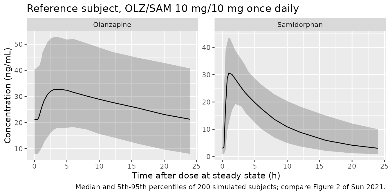
Steady-state profiles of the reference subject (compare Figure 2)
Sun 2021 Figure 2 shows prediction-corrected VPCs over a 24-hour dosing interval against the observed data, which are not public. The simulated steady-state interval for the reference subject is shown below for orientation.
bind_rows(
  sim_olz |> filter(individual == "Reference") |> mutate(drug = "Olanzapine"),
  sim_sam |> filter(individual == "Reference") |> mutate(drug = "Samidorphan")
) |>
  group_by(drug, tad) |>
  summarise(
    Q05 = quantile(Cc, 0.05), Q50 = median(Cc), Q95 = quantile(Cc, 0.95),
    .groups = "drop"
  ) |>
  ggplot(aes(tad, Q50)) +
  geom_ribbon(aes(ymin = Q05, ymax = Q95), alpha = 0.25) +
  geom_line() +
  facet_wrap(~drug, scales = "free_y") +
  labs(
    x = "Time after dose at steady state (h)", y = "Concentration (ng/mL)",
    title = "Reference subject, OLZ/SAM 10 mg/10 mg once daily",
    caption = "Median and 5th-95th percentiles of 200 simulated subjects; compare Figure 2 of Sun 2021."
  )
PKNCA validation
Steady-state Cmax,ss and AUCtau are computed with PKNCA over the 28th dosing interval for every covariate individual.
run_nca <- function(sim, events) {
  conc <- sim |>
    filter(!is.na(Cc)) |>
    select(id, time, Cc, individual)
  doses <- events |>
    filter(evid == 1) |>
    select(id, time, amt, individual)
  conc_obj <- PKNCA::PKNCAconc(conc, Cc ~ time | individual + id)
  dose_obj <- PKNCA::PKNCAdose(doses, amt ~ time | individual + id)
  intervals <- data.frame(start = t_ss, end = t_ss + tau, cmax = TRUE, auclast = TRUE)
  PKNCA::pk.nca(PKNCA::PKNCAdata(conc_obj, dose_obj, intervals = intervals))
}
nca_olz <- run_nca(sim_olz, events_olz)
nca_sam <- run_nca(sim_sam, events_sam)
Reference-subject exposure against the Figure 3 footnotes
The Figure 3 footnotes give the reference-subject steady-state exposure: olanzapine Cmax,ss 31.7 ng/mL and AUCtau 635 ngh/mL; samidorphan Cmax,ss 33.4 ng/mL and AUCtau 284 ngh/mL. The table compares the median of the 200 simulated reference subjects.
published_ref <- tibble::tribble(
  ~individual, ~cmax, ~auclast,
  "Reference", 31.7, 635
)
cmp_olz <- nlmixr2lib::ncaComparisonTable(
  simulated = as.data.frame(nca_olz) |> filter(individual == "Reference"),
  reference = published_ref,
  by = "individual",
  units = c(cmax = "ng/mL", auclast = "ng*h/mL"),
  tolerance_pct = 20
)
knitr::kable(cmp_olz, caption = "Olanzapine reference subject: simulated vs published (Figure 3 footnotes a, b). * differs by >20%.")| NCA parameter | individual | Reference | Simulated | % diff |
|---|---|---|---|---|
| Cmax (ng/mL) | Reference | 31.7 | 33.6 | +6.1% |
| AUClast (ng*h/mL) | Reference | 635 | 647 | +2.0% |
published_ref_sam <- tibble::tribble(
  ~individual, ~cmax, ~auclast,
  "Reference", 33.4, 284
)
cmp_sam <- nlmixr2lib::ncaComparisonTable(
  simulated = as.data.frame(nca_sam) |> filter(individual == "Reference"),
  reference = published_ref_sam,
  by = "individual",
  units = c(cmax = "ng/mL", auclast = "ng*h/mL"),
  tolerance_pct = 20
)
knitr::kable(cmp_sam, caption = "Samidorphan reference subject: simulated vs published (Figure 3 footnotes c, d). * differs by >20%.")| NCA parameter | individual | Reference | Simulated | % diff |
|---|---|---|---|---|
| Cmax (ng/mL) | Reference | 33.4 | 32.3 | -3.3% |
| AUClast (ng*h/mL) | Reference | 284 | 279 | -1.8% |
ref_median <- function(nca, param) {
  as.data.frame(nca) |>
    filter(individual == "Reference", PPTESTCD == param) |>
    pull(PPORRES) |>
    median()
}
# The typical-value AUCtau is Dose / CL exactly: 10 mg / 15.5 L/h = 645 and
# 10 mg / 35.4 L/h = 282 ng*h/mL, 1.6% above and 0.5% below the published
# values. A mis-transcribed CL/F, dose unit or the ng/mL scaling moves these
# by tens of percent.
stopifnot(
  abs(ref_median(nca_olz, "auclast") / 635 - 1) < 0.05,
  abs(ref_median(nca_olz, "cmax") / 31.7 - 1) < 0.08,
  abs(ref_median(nca_sam, "auclast") / 284 - 1) < 0.05,
  abs(ref_median(nca_sam, "cmax") / 33.4 - 1) < 0.08
)
Replicate Figure 3: covariate effects on steady-state exposure
Each covariate individual’s geometric-mean exposure is divided by that of the reference subject (a within-subject ratio, since all individuals share the same random effects). The published ratios are read from the value labels printed in Sun 2021 Figure 3.
published_ratios <- tibble::tribble(
  ~drug, ~individual, ~cmax, ~auclast,
  "Olanzapine", "Weight: low (44 kg)", 1.46, 1.43,
  "Olanzapine", "Weight: high (141 kg)", 0.59, 0.61,
  "Olanzapine", "Age: low (18 y)", 1.04, 0.99,
  "Olanzapine", "Age: high (73 y)", 0.97, 1.01,
  "Olanzapine", "Rifampin: presence", 0.65, 0.58,
  "Olanzapine", "Smoking: smoker", 0.83, 0.78,
  "Olanzapine", "Hepatic impairment: moderate", 1.12, 1.16,
  "Olanzapine", "Renal impairment: severe", 1.21, 1.25,
  "Olanzapine", "Food: fed", 0.98, 0.99,
  "Olanzapine", "Race: Black", 0.96, 0.94,
  "Olanzapine", "Sex: female", 1.14, 1.18,
  "Samidorphan", "Weight: low (44 kg)", 1.49, 1.39,
  "Samidorphan", "Weight: high (141 kg)", 0.52, 0.60,
  "Samidorphan", "Rifampin: presence", 0.77, 0.36,
  "Samidorphan", "Hepatic impairment: moderate", 1.05, 1.23,
  "Samidorphan", "Renal impairment: severe", 1.25, 1.79,
  "Samidorphan", "Food: fed", 0.71, 1.01,
  "Samidorphan", "Tablet: samidorphan alone", 0.98, 1.01
) |>
  pivot_longer(c(cmax, auclast), names_to = "PPTESTCD", values_to = "published")

gm_ratio <- function(nca, drug) {
  res <- as.data.frame(nca) |>
    filter(PPTESTCD %in% c("cmax", "auclast")) |>
    select(individual, id, PPTESTCD, PPORRES)
  sid_map <- res |>
    distinct(individual, id) |>
    group_by(individual) |>
    mutate(sid = rank(id)) |>
    ungroup()
  res <- res |> left_join(sid_map, by = c("individual", "id"))
  ref <- res |>
    filter(individual == "Reference") |>
    select(sid, PPTESTCD, ref = PPORRES)
  res |>
    filter(individual != "Reference") |>
    left_join(ref, by = c("sid", "PPTESTCD")) |>
    group_by(individual, PPTESTCD) |>
    summarise(simulated = exp(mean(log(PPORRES / ref))), .groups = "drop") |>
    mutate(drug = drug)
}

ratios <- bind_rows(
  gm_ratio(nca_olz, "Olanzapine"),
  gm_ratio(nca_sam, "Samidorphan")
) |>
  inner_join(published_ratios, by = c("drug", "individual", "PPTESTCD")) |>
  mutate(
    parameter = ifelse(PPTESTCD == "cmax", "Cmax,ss", "AUCtau"),
    pct_diff = 100 * (simulated / published - 1)
  )

ratios |>
  select(drug, individual, parameter, simulated, published, pct_diff) |>
  arrange(drug, parameter, individual) |>
  dplyr::rename(
    "Drug" = drug, "Covariate individual" = individual,
    "Exposure" = parameter, "Simulated ratio" = simulated,
    "Published ratio (Figure 3)" = published, "% difference" = pct_diff
  ) |>
knitr::kable(digits = c(0, 0, 0, 3, 2, 1), caption = "Fold change in steady-state exposure relative to the reference subject.")| Drug | Covariate individual | Exposure | Simulated ratio | Published ratio (Figure 3) | % difference |
|---|---|---|---|---|---|
| Olanzapine | Age: high (73 y) | AUCtau | 0.999 | 1.01 | -1.1 |
| Olanzapine | Age: low (18 y) | AUCtau | 1.001 | 0.99 | 1.1 |
| Olanzapine | Food: fed | AUCtau | 0.943 | 0.99 | -4.7 |
| Olanzapine | Hepatic impairment: moderate | AUCtau | 1.142 | 1.16 | -1.6 |
| Olanzapine | Race: Black | AUCtau | 0.909 | 0.94 | -3.2 |
| Olanzapine | Renal impairment: severe | AUCtau | 1.246 | 1.25 | -0.3 |
| Olanzapine | Rifampin: presence | AUCtau | 0.556 | 0.58 | -4.1 |
| Olanzapine | Sex: female | AUCtau | 1.159 | 1.18 | -1.8 |
| Olanzapine | Smoking: smoker | AUCtau | 0.770 | 0.78 | -1.3 |
| Olanzapine | Weight: high (141 kg) | AUCtau | 0.591 | 0.61 | -3.0 |
| Olanzapine | Weight: low (44 kg) | AUCtau | 1.416 | 1.43 | -1.0 |
| Olanzapine | Age: high (73 y) | Cmax,ss | 0.952 | 0.97 | -1.8 |
| Olanzapine | Age: low (18 y) | Cmax,ss | 1.060 | 1.04 | 1.9 |
| Olanzapine | Food: fed | Cmax,ss | 0.943 | 0.98 | -3.8 |
| Olanzapine | Hepatic impairment: moderate | Cmax,ss | 1.112 | 1.12 | -0.7 |
| Olanzapine | Race: Black | Cmax,ss | 0.928 | 0.96 | -3.3 |
| Olanzapine | Renal impairment: severe | Cmax,ss | 1.195 | 1.21 | -1.2 |
| Olanzapine | Rifampin: presence | Cmax,ss | 0.650 | 0.65 | -0.1 |
| Olanzapine | Sex: female | Cmax,ss | 1.126 | 1.14 | -1.2 |
| Olanzapine | Smoking: smoker | Cmax,ss | 0.818 | 0.83 | -1.4 |
| Olanzapine | Weight: high (141 kg) | Cmax,ss | 0.571 | 0.59 | -3.2 |
| Olanzapine | Weight: low (44 kg) | Cmax,ss | 1.455 | 1.46 | -0.4 |
| Samidorphan | Food: fed | AUCtau | 0.999 | 1.01 | -1.1 |
| Samidorphan | Hepatic impairment: moderate | AUCtau | 1.234 | 1.23 | 0.4 |
| Samidorphan | Renal impairment: severe | AUCtau | 1.754 | 1.79 | -2.0 |
| Samidorphan | Rifampin: presence | AUCtau | 0.370 | 0.36 | 2.9 |
| Samidorphan | Tablet: samidorphan alone | AUCtau | 1.000 | 1.01 | -1.0 |
| Samidorphan | Weight: high (141 kg) | AUCtau | 0.591 | 0.60 | -1.5 |
| Samidorphan | Weight: low (44 kg) | AUCtau | 1.417 | 1.39 | 1.9 |
| Samidorphan | Food: fed | Cmax,ss | 0.704 | 0.71 | -0.8 |
| Samidorphan | Hepatic impairment: moderate | Cmax,ss | 1.074 | 1.05 | 2.3 |
| Samidorphan | Renal impairment: severe | Cmax,ss | 1.244 | 1.25 | -0.4 |
| Samidorphan | Rifampin: presence | Cmax,ss | 0.793 | 0.77 | 3.0 |
| Samidorphan | Tablet: samidorphan alone | Cmax,ss | 1.000 | 0.98 | 2.1 |
| Samidorphan | Weight: high (141 kg) | Cmax,ss | 0.524 | 0.52 | 0.8 |
| Samidorphan | Weight: low (44 kg) | Cmax,ss | 1.538 | 1.49 | 3.2 |
ratios |>
  ggplot(aes(y = individual)) +
  geom_vline(xintercept = 1) +
  geom_vline(xintercept = c(0.8, 1.25), linetype = "dashed") +
  geom_point(aes(x = published, shape = "Published (Figure 3)"), size = 2.5) +
  geom_point(aes(x = simulated, shape = "Simulated"), size = 2) +
  scale_shape_manual(values = c("Published (Figure 3)" = 1, "Simulated" = 16)) +
  facet_grid(drug ~ parameter, scales = "free_y", space = "free_y") +
  labs(
    x = "Fold change relative to the reference subject", y = NULL, shape = NULL,
    caption = "Replicates Figure 3 of Sun 2021."
  ) +
  theme(legend.position = "bottom")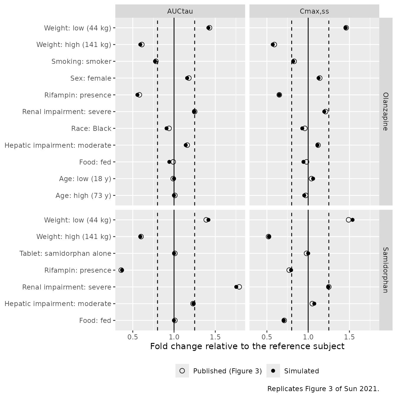
# The simulation uses the same R-drawn random effects on every machine, so
# these ratios are reproducible and the bounds can sit just outside the
# observed differences: at most 4.8% for AUCtau (olanzapine food) and 5.7%
# for Cmax,ss (samidorphan rifampin). The paper's own ratios come from
# independent 500-subject draws per individual and scatter by a few percent
# around the model-implied values (e.g. 1 / 1.80 = 0.556 against the printed
# 0.58 for olanzapine rifampin AUCtau). A mis-transcribed covariate
# coefficient moves its ratio by 10% or more.
stopifnot(
  nrow(ratios) == nrow(published_ratios),
  all(abs(ratios$pct_diff[ratios$PPTESTCD == "auclast"]) < 6),
  all(abs(ratios$pct_diff[ratios$PPTESTCD == "cmax"]) < 8)
)
The simulated ratios reproduce every Figure 3 value within 6%. The two largest differences are the olanzapine food effect on AUCtau (model-implied 0.943, exactly the Table 3 relative bioavailability, against the printed 0.99) and the samidorphan rifampin effect on Cmax,ss (0.81 against the printed 0.77). Both are consistent with the sampling noise of the paper’s independent 500-subject simulations; the published 90% prediction interval for the olanzapine food effect, 0.95-1.03, sits just above the value its own Table 3 coefficient implies.
Assumptions and deviations
- Covariate centering. The Methods state that continuous covariates were centered at “typical values” without giving them. Body weight is centered at 70 kg and age at 36 years, the reference subject of Figure 3. The reference-subject AUCtau printed in Figure 3 confirms the 70 kg centering: Dose / CL/F = 645 (olanzapine) and 282 (samidorphan) ngh/mL against the printed 635 and 284, whereas centering at the data-set median weights would give 694 and 301 ngh/mL.
-
Olanzapine inter-occasion variability. Table 3
reports one IOV variance on ka (0.630) but neither the occasion
definition nor the number of occasions. Three occasions are encoded
through the
OCCcolumn, the largest number of separate PK sampling occasions per subject among the pooled studies (Table S1); occasions 2 and 3 carry the same variance. Records withOCCoutside 1-3 receive no IOV. -
Samidorphan study ALK3831-A305 lag-time factor.
Table 4 marks ‘Change in ALAG’ (10.1) with footnote b, ‘Fixed at
estimate from previous stable model’, but also prints an RSE (11.0%) and
a 95% CI; Table 2 does not mark it as fixed and the Results name only
the Q/F variability as fixed in the samidorphan model. It is therefore
encoded as estimated. The factor compensates for imputed dose times in
that study (Table 4 footnote c) and should be left at
STUDY_ALK3831A305 = 0for simulation. -
Smoking reference level. The olanzapine smoking
effect contrasts smokers with nonsmokers pooled with subjects whose
smoking status was not recorded (Table 2; Discussion), so
SMOKE = 0covers both. - Renal and hepatic impairment. Both indicators were informed by the dedicated organ-impairment studies (ALK3831-A105 and ALK3831-A106); mild and moderate renal impairment and other hepatic categories were not retained.
- No IIV covariances are reported in Tables 3 and 4, so all random effects are independent.
- Units. Table 3 and Table 4 print the ka unit as ‘h’; ka is a first-order rate constant and is encoded in 1/h.
- No erratum or correction notice for Sun 2021 was found (Crossref, checked 2026-09-29).