Moxifloxacin (Palmer 2025)
Source:vignettes/articles/Palmer_2025_moxifloxacin.Rmd
Palmer_2025_moxifloxacin.RmdModel and source
- Citation: Palmer M, Zou Y, Hesseling AC, van der Laan L, Courtney I, Kinikar AA, Sonkawade N, Paradkar M, Kulkarni V, Casalme DJO, Frias MVG, Draper H, Wiesner L, Karlsson MO, Denti P, Svensson EM, Garcia-Prats AJ. Population pharmacokinetics and dosing of dispersible moxifloxacin formulation in children with rifampicin-resistant tuberculosis. Br J Clin Pharmacol. 2025;91(6):1853-1864. doi:10.1002/bcp.70005. Structural model adapted from Radtke KK et al., Clin Infect Dis. 2022;74(8):1372-1381.
- Description: Two-compartment population PK model with a four-step first-order transit-chain absorption for oral moxifloxacin in children with rifampicin-resistant tuberculosis (Palmer 2025, CATALYST trial). Apparent disposition parameters are allometrically scaled on body weight to a 16 kg reference child with fixed exponents 0.75 (CL/F, Q/F) and 1 (Vc/F, Vp/F); bioavailability is fixed to 1 because only oral data were available. Interindividual variability is carried on CL/F alone, while interoccasion variability sits on bioavailability and on the mean absorption time MAT, with the IOV magnitude inflated 1.70-fold on dosing occasions that were not directly observed. A dispersible 100 mg paediatric tablet and the standard crushed 400 mg adult tablet were found bioequivalent, so the final model carries no formulation term.
- Article: https://doi.org/10.1002/bcp.70005
- Supplement (Supplementary Material 1-9, including the final NONMEM control stream in Supplementary Material 9): https://europepmc.org/article/PMC/PMC12122143
Population
CATALYST was an open-label multisite trial of child-friendly generic formulations of moxifloxacin and clofazimine (Pan African Clinical Trials Registry 202012756409365). Thirty-six children being treated for rifampicin-resistant tuberculosis were enrolled across three sites: South Africa (n = 20), the Philippines (n = 10) and India (n = 6). Median age was 4.8 years (range 0.4-15) and median weight 15.6 kg (range 6.9-42.1); enrolment was stratified into two parallel weight cohorts so that 16 children weighed under 15 kg, of whom 6 weighed under 10 kg. Fourteen (39%) were male. Median height-for-age z-score was -1.1 (range -4.1 to 0.46) and median weight-for-age z-score -1.6 (range -4.7 to 1.2). Tuberculosis was microbiologically confirmed in 17 (47.2%). Only one child (3%) was living with HIV (Table 1).
Each child was sampled intensively twice. At visit PK1 they were taking the standard non-dispersible 400 mg adult tablet, crushed and suspended in water; at visit PK2, one to fourteen days later, they took their first dose of the dispersible 100 mg scored paediatric tablet, dispersed in water. Samples were drawn predose and at 1, 2, 4, 8 and 24 h postdose on each visit day, with children fasted for at least 4 h before the predose draw and then given breakfast before dosing. Doses followed the WHO weight-band recommendations (Methods 2.1.3). Moxifloxacin was assayed by validated LC-MS/MS with an LLOQ of 0.0628 ug/mL.
The same information is available programmatically via the model’s
population metadata
(readModelDb("Palmer_2025_moxifloxacin")()$population).
Source trace
The per-parameter origin is recorded as an in-file comment next to
each ini() entry in
inst/modeldb/specificDrugs/Palmer_2025_moxifloxacin.R. The
table below collects them in one place for review. Every number below
was read from the Palmer 2025 main article; the model structure
was confirmed against the final NONMEM control stream printed in
Supplementary Material 9.
| Equation / parameter | Value | Source location |
|---|---|---|
lcl |
log(6.90 L/h) | Table 2, CL/F (L/h)
|
lvc |
log(61.1 L) | Table 2, Vc/F (L)
|
lq |
log(0.860 L/h) | Table 2, Q/F (L/h)
|
lvp |
log(44.5 L) | Table 2, Vp/F (L)
|
lmat |
log(1.01 h) | Table 2, MAT (h)
|
lfdepot |
fixed(log(1)) | Table 2, F = 1 (fixed); footnote a |
e_wt_cl |
fixed(0.75) | Table 2 footnote a (exponent for CL and Q) |
e_wt_vc |
fixed(1.0) | Table 2 footnote a (exponent for Vc and Vp) |
e_selfadmin_iovscale |
1.70 | Table 2,
Fold change of unobserved dosing event on IOV of F and MAT
|
etalcl |
0.136^2 = 0.018496 | Table 2, IIV on CL (%CV) = 13.6; footnote c defines %CV
as sqrt(variance) * 100%
|
etaiov_fdepot_1..4 |
0.308^2 = 0.094864 | Table 2, IOV on F (%CV) = 30.8; footnote c |
etaiov_mat_1..4 |
0.422^2 = 0.178084 | Table 2, IOV on MAT (%CV) = 42.2; footnote c |
propSd |
0.136 | Table 2, Proportional error (%) = 13.6; footnote c |
addSd |
0.0435 mg/L | Table 2, Additive error (mg/L); footnote d, “reported
in the standard deviation scale” |
Allometry (WT/16)^theta on CL, Q, Vc, Vp |
n/a | Table 2 footnote a |
ktr = 4 / mat;
depot -> transit1 -> transit2 -> transit3 -> central
|
n/a | Supplementary Material 9 $PK: KTR = 4/MAT,
K14 = K45 = K56 = K62 = KTR;
$MODEL NCOMP=6 COMP=(DOS,DEFDOSE) COMP=(MOXC,DEFOBS) COMP=(MOXP) COMP=(TRANSI) COMP=(TRANSI2) COMP=(TRANSI3);
Results paragraph 2 (“absorption via 3 transit compartments and
estimating mean absorption time”) |
k12 = q/vc, k21 = q/vp,
kel = cl/vc
|
n/a | Supplementary Material 9 $PK: K23 = Q/V2,
K32 = Q/V3, K20 = CL/V2
|
f(depot) = exp(lfdepot + iov_fdepot) |
n/a | Supplementary Material 9 $PK:
F1 = 1 * EXP(IOVF * UNOBS_EFF)
|
mat = exp(lmat + iov_mat);
iov_*_scale = 1.70^SELFADMIN
|
n/a | Supplementary Material 9 $PK:
UNOBS_EFF = 1 + THETA(10)*UNOBS,
MAT = TVMAT * EXP(IOVMAT * UNOBS_EFF)
|
Cc ~ add(addSd) + prop(propSd) |
n/a | Supplementary Material 9 $ERROR:
Y = IPRED + IPRED*EPS(1) + EPS(2)
|
The final model carries no formulation term: the dispersible-versus-standard ratios on bioavailability (1.05, 90% CI 0.95-1.15) and on MAT (1.06, 90% CI 0.90-1.26) were not significant, and Table 2 has no formulation row.
mod <- readModelDb("Palmer_2025_moxifloxacin")
th <- rxode2::rxode(mod)$theta
#> ℹ parameter labels from comments will be replaced by 'label()'
#> Warning: some etas defaulted to non-mu referenced, possible parsing error: etaiov_fdepot_1, etaiov_fdepot_2, etaiov_fdepot_3, etaiov_fdepot_4, etaiov_mat_1, etaiov_mat_2, etaiov_mat_3, etaiov_mat_4
#> as a work-around try putting the mu-referenced expression on a simple line
mod_typical <- rxode2::zeroRe(mod)
#> ℹ parameter labels from comments will be replaced by 'label()'
#> Warning: some etas defaulted to non-mu referenced, possible parsing error: etaiov_fdepot_1, etaiov_fdepot_2, etaiov_fdepot_3, etaiov_fdepot_4, etaiov_mat_1, etaiov_mat_2, etaiov_mat_3, etaiov_mat_4
#> as a work-around try putting the mu-referenced expression on a simple line
#> Warning: some etas defaulted to non-mu referenced, possible parsing error: etaiov_fdepot_1, etaiov_fdepot_2, etaiov_fdepot_3, etaiov_fdepot_4, etaiov_mat_1, etaiov_mat_2, etaiov_mat_3, etaiov_mat_4
#> as a work-around try putting the mu-referenced expression on a simple line

tau <- 24      # once-daily dosing interval, h
n_dose <- 12   # doses simulated to reach steady state
t_end <- tau * n_dose
Structural checks
Three relationships in this paper are exact arithmetic on the packaged parameters rather than statements about a simulated cohort, so they can be checked to numerical precision.
Table 4 dose ratios
The paper states that, relative to the WHO recommendations, the proposed doses were “adjusted upwards by 50-56% in 5-7 kg for both formulations and 33% in 7-10 kg for standard formulation; doses in children >10 kg remained the same as WHO recommended”. That is pure arithmetic on Table 4 and must reproduce exactly.
# Palmer 2025 Table 4, daily dose in mg by WHO weight band.
table4 <- tibble::tibble(
  band = factor(rep(c("5-<7", "7-<10", "10-<16", "16-<24", ">=24"), 2),
                levels = c("5-<7", "7-<10", "10-<16", "16-<24", ">=24")),
  formulation = rep(c("Standard 400 mg", "Dispersible 100 mg"), each = 5),
  # Band midpoints; the top band is simulated over 24-31 kg because Results 3.2
  # notes the >=25 kg recommendation equals the 400 mg adult dose.
  wt_lo = rep(c(5, 7, 10, 16, 24), 2),
  wt_hi = rep(c(7, 10, 16, 24, 31), 2),
  who   = c(80, 120, 200, 300, 400,
            80, 150, 200, 300, 400),
  proposed = c(120, 160, 200, 300, 400,
               125, 150, 200, 300, 400)
) |>
  dplyr::mutate(pct_increase = 100 * (proposed / who - 1))

knitr::kable(
  table4 |>
    dplyr::select(`Weight band (kg)` = band, Formulation = formulation,
                  `WHO dose (mg)` = who, `Proposed dose (mg)` = proposed,
                  `Increase (%)` = pct_increase),
  digits = 2,
  caption = "Palmer 2025 Table 4: WHO and proposed daily moxifloxacin doses."
)| Weight band (kg) | Formulation | WHO dose (mg) | Proposed dose (mg) | Increase (%) |
|---|---|---|---|---|
| 5-<7 | Standard 400 mg | 80 | 120 | 50.00 |
| 7-<10 | Standard 400 mg | 120 | 160 | 33.33 |
| 10-<16 | Standard 400 mg | 200 | 200 | 0.00 |
| 16-<24 | Standard 400 mg | 300 | 300 | 0.00 |
| >=24 | Standard 400 mg | 400 | 400 | 0.00 |
| 5-<7 | Dispersible 100 mg | 80 | 125 | 56.25 |
| 7-<10 | Dispersible 100 mg | 150 | 150 | 0.00 |
| 10-<16 | Dispersible 100 mg | 200 | 200 | 0.00 |
| 16-<24 | Dispersible 100 mg | 300 | 300 | 0.00 |
| >=24 | Dispersible 100 mg | 400 | 400 | 0.00 |
low_band <- table4$pct_increase[table4$band == "5-<7"]
std_7_10 <- table4$pct_increase[table4$band == "7-<10" &
                                  table4$formulation == "Standard 400 mg"]
big_bands <- table4$pct_increase[table4$wt_lo >= 10]

stopifnot(
  # "adjusted upwards by 50-56% in 5-7 kg for both formulations"
  all(low_band >= 50 & low_band <= 56.5),
  # "and 33% in 7-10 kg for standard formulation"
  abs(std_7_10 - 33) < 1,
  # "doses in children >10 kg remained the same as WHO recommended"
  all(big_bands == 0)
)
Steady-state AUC equals dose divided by clearance
The paper derives every simulated exposure from
AUC0-24,ss = (Dose * Bioavailability) / Clearance (Methods
2.3). Because bioavailability is fixed at 1 and the model is linear, a
steady-state interval of the solved ODE system must reproduce that
closed form. Both sides use the same parameter values here (random
effects are zeroed), so the only difference is trapezoidal integration
error and the bound can be tight.
typical_events <- function(wt, dose, occ = 2, selfadmin = 0, by = 0.05) {
  dosing <- tibble::tibble(
    id = 1L, time = seq(0, tau * (n_dose - 1), by = tau),
    amt = dose, evid = 1L, cmt = "depot"
  )
  obs <- tibble::tibble(
    id = 1L, time = seq(t_end - tau, t_end, by = by),
    amt = NA_real_, evid = 0L, cmt = "central"
  )
  dplyr::bind_rows(dosing, obs) |>
    dplyr::mutate(WT = wt, OCC = occ, SELFADMIN = selfadmin) |>
    dplyr::arrange(id, time, dplyr::desc(evid))
}

trapz <- function(x, y) sum(diff(x) * (utils::head(y, -1) + utils::tail(y, -1)) / 2)

wt_check <- 15.6   # cohort median weight, Table 1
dose_check <- 200  # WHO dose for the 10-<16 kg band, Table 4

sim_cf <- rxode2::rxSolve(mod_typical, typical_events(wt_check, dose_check),
                          omega = NA, sigma = NA) |>
  as.data.frame() |>
  dplyr::filter(time >= t_end - tau)

auc_solved <- trapz(sim_cf$time, sim_cf$Cc)
cl_check <- exp(th[["lcl"]]) * (wt_check / 16)^th[["e_wt_cl"]]
auc_closed <- dose_check * exp(th[["lfdepot"]]) / cl_check

cat(sprintf("solved AUC(0-24,ss) = %.4f mg*h/L; Dose/CL = %.4f mg*h/L; ratio = %.5f\n",
            auc_solved, auc_closed, auc_solved / auc_closed))
#> solved AUC(0-24,ss) = 29.5078 mg*h/L; Dose/CL = 29.5412 mg*h/L; ratio = 0.99887

# Realised ratio 0.99887. Two deterministic sources of the shortfall: the deep
# peripheral compartment (Q/F = 0.860 L/h into Vp/F = 44.5 L) has not fully
# equilibrated after 12 daily doses, and the linear trapezoid under-reads a
# peaked profile. Neither depends on the random draw or the thread count. A
# mis-transcribed CL, reference weight or allometric exponent moves this by tens
# of percent, so 0.5% is still a live gate.
stopifnot(abs(auc_solved / auc_closed - 1) < 0.005)
The transit chain is actually driving absorption
cl / vc parameter pairs can make rxode2
substitute a solved linear compartment model and silently discard an
explicitly written ODE system. If that happened here the four-step
transit chain would be gone and absorption would no longer depend on MAT
at all. Quadrupling MAT must therefore move Tmax substantially, and the
transit states must appear in the solved output.
mod_slow <- mod |> rxode2::ini(lmat = log(4 * 1.01)) |> rxode2::zeroRe()
#> ℹ parameter labels from comments will be replaced by 'label()'
#> Warning: some etas defaulted to non-mu referenced, possible parsing error: etaiov_fdepot_1, etaiov_fdepot_2, etaiov_fdepot_3, etaiov_fdepot_4, etaiov_mat_1, etaiov_mat_2, etaiov_mat_3, etaiov_mat_4
#> as a work-around try putting the mu-referenced expression on a simple line
#> ℹ change initial estimate of `lmat` to `1.39624469197306`
#> Warning: some etas defaulted to non-mu referenced, possible parsing error: etaiov_fdepot_1, etaiov_fdepot_2, etaiov_fdepot_3, etaiov_fdepot_4, etaiov_mat_1, etaiov_mat_2, etaiov_mat_3, etaiov_mat_4
#> as a work-around try putting the mu-referenced expression on a simple line

tmax_of <- function(m) {
  s <- rxode2::rxSolve(m, typical_events(wt_check, dose_check),
                       omega = NA, sigma = NA) |>
    as.data.frame() |>
    dplyr::filter(time >= t_end - tau)
  list(tmax = s$time[which.max(s$Cc)] - (t_end - tau),
       cmax = max(s$Cc),
       states = names(s))
}

base_p <- tmax_of(mod_typical)
slow_p <- tmax_of(mod_slow)

cat(sprintf("MAT = 1.01 h: Tmax = %.2f h, Cmax = %.3f mg/L\n", base_p$tmax, base_p$cmax))
#> MAT = 1.01 h: Tmax = 2.00 h, Cmax = 3.083 mg/L
cat(sprintf("MAT = 4.04 h: Tmax = %.2f h, Cmax = %.3f mg/L\n", slow_p$tmax, slow_p$cmax))
#> MAT = 4.04 h: Tmax = 6.20 h, Cmax = 2.322 mg/L

stopifnot(
  # The transit chain exists as ODE states in the solved output.
  all(c("depot", "transit1", "transit2", "transit3", "central", "peripheral1") %in%
        base_p$states),
  # Absorption really is MAT-driven: realised 2.00 h -> 6.20 h.
  slow_p$tmax - base_p$tmax > 2,
  # And slower absorption flattens the peak: realised 3.08 -> 2.32 mg/L.
  slow_p$cmax < base_p$cmax
)
Tmax at the published MAT is 2.0 h, against the median Tmax of 2.1 h that Palmer 2025 Table 3 reports for the trial participants.
Virtual cohort
Original observed data are not publicly available. Two virtual cohorts are used below, both capped at 200 participants per arm.
- A CATALYST-like cohort for the Table 3 comparison: 200 children with weights drawn from a log-normal truncated to the observed 6.9-42.1 kg range and centred on the observed median of 15.6 kg, half dosed on the standard and half on the dispersible formulation at the WHO weight-band doses of Table 4. The paper does not publish the weight distribution beyond its median and range, so the log-normal shape is an assumption (see Errata).
- A dosing-simulation cohort replicating the paper’s Figure 4: for each WHO weight band, weight is drawn uniformly across the band, exactly as Results 3.2 describes (“Uniformly distributed body weight … from 5 to 31 kg was applied in the population simulation”).
Both cohorts use OCC values corresponding to directly
observed clinic doses, so SELFADMIN = 0 and the
interoccasion variability is not inflated. The unobserved-dosing arm is
exercised separately in its own section below.
# set.seed() seeds R's RNG (used for the weight draws). It does NOT seed
# rxode2's simulation RNG, whose streams are partitioned per solver thread, so
# the etas differ between a 2-thread CI runner and a 16-thread workstation.
# Every assertion below is therefore written to hold for any cohort this model
# can produce.
set.seed(20250523)
n_per_arm <- 200

who_dose <- function(wt, dispersible) {
  dplyr::case_when(
    wt < 7             ~ 80,
    wt < 10            ~ dplyr::if_else(dispersible, 150, 120),
    wt < 16            ~ 200,
    wt < 24            ~ 300,
    TRUE               ~ 400
  )
}

catalyst <- tibble::tibble(
  id = seq_len(n_per_arm),
  WT = pmin(pmax(exp(stats::rnorm(n_per_arm, log(15.6), 0.45)), 6.9), 42.1),
  dispersible = rep(c(FALSE, TRUE), length.out = n_per_arm)
) |>
  dplyr::mutate(
    dose = who_dose(WT, dispersible),
    # OCC 2 = observed standard-formulation dose at the PK1 visit,
    # OCC 4 = observed dispersible-formulation dose at the PK2 visit.
    OCC = dplyr::if_else(dispersible, 4, 2),
    SELFADMIN = 0,
    arm = dplyr::if_else(dispersible, "Scored dispersible tablet", "Nondispersible tablet")
  )

expand_events <- function(subjects, obs_by = 0.1) {
  dosing <- subjects |>
    dplyr::select(id, WT, OCC, SELFADMIN, arm, dose) |>
    tidyr::expand_grid(time = seq(0, tau * (n_dose - 1), by = tau)) |>
    dplyr::mutate(amt = dose, evid = 1L, cmt = "depot") |>
    dplyr::select(-dose)
  obs <- subjects |>
    dplyr::select(id, WT, OCC, SELFADMIN, arm) |>
    tidyr::expand_grid(time = seq(t_end - tau, t_end, by = obs_by)) |>
    dplyr::mutate(amt = NA_real_, evid = 0L, cmt = "central")
  dplyr::bind_rows(dosing, obs) |>
    dplyr::arrange(id, time, dplyr::desc(evid))
}

catalyst_events <- expand_events(catalyst)
stopifnot(!anyDuplicated(catalyst_events[, c("id", "time", "evid")]))
Simulation
sim <- rxode2::rxSolve(mod, events = catalyst_events, keep = c("WT", "arm")) |>
  as.data.frame()
#> ℹ parameter labels from comments will be replaced by 'label()'
#> Warning: some etas defaulted to non-mu referenced, possible parsing error: etaiov_fdepot_1, etaiov_fdepot_2, etaiov_fdepot_3, etaiov_fdepot_4, etaiov_mat_1, etaiov_mat_2, etaiov_mat_3, etaiov_mat_4
#> as a work-around try putting the mu-referenced expression on a simple line

stopifnot(dplyr::n_distinct(sim$id) == n_per_arm)

# Time after dose within the final, steady-state, dosing interval.
sim_ss <- sim |>
  dplyr::filter(time >= t_end - tau) |>
  dplyr::mutate(tad = time - (t_end - tau))
Replicate published figures
band_profile <- sim_ss |>
  dplyr::group_by(arm, tad) |>
  dplyr::summarise(
    lo = stats::quantile(Cc, 0.05),
    md = stats::quantile(Cc, 0.50),
    hi = stats::quantile(Cc, 0.95),
    .groups = "drop"
  )

ggplot(band_profile, aes(tad, md)) +
  geom_ribbon(aes(ymin = lo, ymax = hi), alpha = 0.2) +
  geom_line(linewidth = 0.8) +
  facet_wrap(~arm) +
  labs(x = "Time after dose (h)", y = "Moxifloxacin concentration (mg/L)",
       title = "Steady-state profiles, WHO weight-band dosing",
       caption = "Median with 5th-95th percentile band. Figure 2 of Palmer 2025 shows the observed VPC separated by formulation.")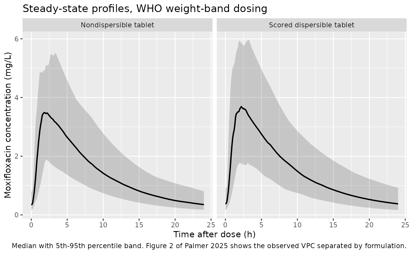
Steady-state concentration-time profiles by formulation, in the style of Figure 2 of Palmer 2025.
The two formulations overlay almost exactly, which is the model’s structural consequence of the paper finding no significant formulation effect on either bioavailability or MAT.
# Replicates the simulation design of Palmer 2025 Figure 4: for each WHO weight
# band, weight is uniform across the band and the band's dose is taken from
# Table 4, once for the WHO dosing table and once for the proposed one.
set.seed(20250524)
n_band <- 100  # per band x dosing-table x formulation arm

band_cohort <- table4 |>
  dplyr::select(band, formulation, wt_lo, wt_hi, who, proposed) |>
  tidyr::pivot_longer(c(who, proposed), names_to = "dosing_table", values_to = "dose") |>
  dplyr::mutate(dosing_table = dplyr::recode(dosing_table,
                                             who = "WHO", proposed = "Proposed")) |>
  dplyr::mutate(arm_id = dplyr::row_number()) |>
  tidyr::expand_grid(k = seq_len(n_band)) |>
  dplyr::mutate(
    id = (arm_id - 1L) * n_band + k,
    WT = stats::runif(dplyr::n(), wt_lo, wt_hi),
    OCC = 2, SELFADMIN = 0,
    arm = paste(formulation, dosing_table, band, sep = " | ")
  )

band_sim <- rxode2::rxSolve(
  mod, events = expand_events(band_cohort, obs_by = 0.25),
  keep = c("WT", "arm")
) |>
  as.data.frame() |>
  dplyr::filter(time >= t_end - tau)

band_metrics <- band_sim |>
  dplyr::group_by(id, arm) |>
  dplyr::summarise(auc = trapz(time, Cc), cmax = max(Cc), .groups = "drop") |>
  tidyr::separate(arm, into = c("formulation", "dosing_table", "band"),
                  sep = " \\| ") |>
  dplyr::mutate(band = factor(band, levels = levels(table4$band)),
                dosing_table = factor(dosing_table, levels = c("WHO", "Proposed")))
# Aggregated adult reference exposures, Palmer 2025 Figure 4 caption and
# Supplementary Material 6: AUC0-24,ss median 37 (15-76) mg*h/L, Cmax median
# 3.06 (1.36-6.72) mg/L.
ref <- list(auc = c(lo = 15, md = 37, hi = 76),
            cmax = c(lo = 1.36, md = 3.06, hi = 6.72))

band_long <- band_metrics |>
  tidyr::pivot_longer(c(auc, cmax), names_to = "metric", values_to = "value") |>
  dplyr::mutate(metric = dplyr::recode(
    metric,
    auc = "AUC(0-24,ss) (mg*h/L)", cmax = "Cmax (mg/L)"
  ))

ref_df <- tibble::tibble(
  metric = c("AUC(0-24,ss) (mg*h/L)", "Cmax (mg/L)"),
  lo = c(ref$auc[["lo"]], ref$cmax[["lo"]]),
  md = c(ref$auc[["md"]], ref$cmax[["md"]]),
  hi = c(ref$auc[["hi"]], ref$cmax[["hi"]])
)

ggplot(band_long, aes(band, value, fill = dosing_table)) +
  geom_rect(data = ref_df, inherit.aes = FALSE,
            aes(xmin = -Inf, xmax = Inf, ymin = lo, ymax = hi),
            fill = "red", alpha = 0.10) +
  geom_hline(data = ref_df, aes(yintercept = md), colour = "red") +
  geom_boxplot(outlier.size = 0.4, coef = 0) +
  facet_grid(metric ~ formulation, scales = "free_y") +
  labs(x = "WHO weight band (kg)", y = NULL, fill = "Dosing table",
       title = "Simulated steady-state exposures by weight band",
       caption = paste("Red line: aggregated adult reference median.",
                       "Shaded: adult 2.5th-97.5th percentile range.")) +
  theme(legend.position = "bottom",
        axis.text.x = element_text(angle = 30, hjust = 1))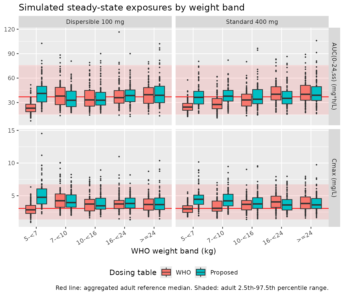
Replicates Figure 4 of Palmer 2025.
Gating the paper’s dosing conclusions
Palmer 2025 concludes that “WHO-recommended doses yielded AUC0-24,ss
similar to those in adults for children >10 kg, but that the median
AUC0-24,ss in the smallest children were considerably below the adult
reference median”, and that the proposed doses were chosen “to produce
median AUC0-24,ss closest to the reference median”. Because
bioavailability is fixed and the model is linear, the typical exposure
in each band is exactly Dose / CL(WT), so these claims can
be checked deterministically at the band midpoints without relying on a
drawn cohort.
band_typical <- table4 |>
  dplyr::mutate(
    wt_mid = (wt_lo + wt_hi) / 2,
    cl = exp(th[["lcl"]]) * (wt_mid / 16)^th[["e_wt_cl"]],
    auc_who = who / cl,
    auc_proposed = proposed / cl,
    pct_who = 100 * (auc_who / ref$auc[["md"]] - 1),
    pct_proposed = 100 * (auc_proposed / ref$auc[["md"]] - 1)
  )

knitr::kable(
  band_typical |>
    dplyr::select(`Weight band (kg)` = band, Formulation = formulation,
                  `Midpoint WT (kg)` = wt_mid,
                  `AUC, WHO dose (mg*h/L)` = auc_who,
                  `WHO vs adult median (%)` = pct_who,
                  `AUC, proposed dose (mg*h/L)` = auc_proposed,
                  `Proposed vs adult median (%)` = pct_proposed),
  digits = 1,
  caption = paste("Typical steady-state AUC0-24 by weight band against the",
                  "aggregated adult reference median of 37 mg*h/L.")
)| Weight band (kg) | Formulation | Midpoint WT (kg) | AUC, WHO dose (mg*h/L) | WHO vs adult median (%) | AUC, proposed dose (mg*h/L) | Proposed vs adult median (%) |
|---|---|---|---|---|---|---|
| 5-<7 | Standard 400 mg | 6.0 | 24.2 | -34.6 | 36.3 | -1.9 |
| 7-<10 | Standard 400 mg | 8.5 | 27.9 | -24.5 | 37.3 | 0.7 |
| 10-<16 | Standard 400 mg | 13.0 | 33.9 | -8.5 | 33.9 | -8.5 |
| 16-<24 | Standard 400 mg | 20.0 | 36.8 | -0.6 | 36.8 | -0.6 |
| >=24 | Standard 400 mg | 27.5 | 38.6 | 4.4 | 38.6 | 4.4 |
| 5-<7 | Dispersible 100 mg | 6.0 | 24.2 | -34.6 | 37.8 | 2.2 |
| 7-<10 | Dispersible 100 mg | 8.5 | 34.9 | -5.6 | 34.9 | -5.6 |
| 10-<16 | Dispersible 100 mg | 13.0 | 33.9 | -8.5 | 33.9 | -8.5 |
| 16-<24 | Dispersible 100 mg | 20.0 | 36.8 | -0.6 | 36.8 | -0.6 |
| >=24 | Dispersible 100 mg | 27.5 | 38.6 | 4.4 | 38.6 | 4.4 |
stopifnot(
  # Every proposed dose lands the typical child near the adult reference median.
  # Realised range -8.5% to +4.4%; 15% still breaks on a mis-transcribed CL,
  # reference weight or allometric exponent, which move AUC by tens of percent.
  all(abs(band_typical$pct_proposed) < 15),
  # WHO dosing is adequate above 10 kg ...
  all(abs(band_typical$pct_who[band_typical$wt_lo >= 10]) < 15),
  # ... and underdoses below 10 kg. Realised -34.6% (5-<7 kg, both
  # formulations), -24.5% (7-<10 kg standard), -5.6% (7-<10 kg dispersible),
  # which is why the paper proposes a dose increase for the standard
  # formulation in 7-<10 kg but not for the dispersible one.
  all(band_typical$pct_who[band_typical$band == "5-<7"] < -20),
  band_typical$pct_who[band_typical$band == "7-<10" &
                         band_typical$formulation == "Standard 400 mg"] < -15
)
PKNCA validation
nca_conc <- sim_ss |>
  dplyr::filter(!is.na(Cc)) |>
  dplyr::select(id, arm, tad, Cc)

nca_dose <- catalyst |>
  dplyr::mutate(tad = 0) |>
  dplyr::select(id, arm, tad, dose)

conc_obj <- PKNCA::PKNCAconc(nca_conc, Cc ~ tad | arm + id,
                             concu = "mg/L", timeu = "h")
dose_obj <- PKNCA::PKNCAdose(nca_dose, dose ~ tad | arm + id, doseu = "mg")

intervals <- data.frame(
  start = 0, end = tau,
  auclast = TRUE, cmax = TRUE, tmax = TRUE
)

nca_res <- PKNCA::pk.nca(PKNCA::PKNCAdata(conc_obj, dose_obj,
                                          intervals = intervals))
nca_df <- as.data.frame(nca_res)

stopifnot(nrow(nca_df) > 0, dplyr::n_distinct(nca_df$id) == n_per_arm)
Comparison against published NCA
Palmer 2025 Table 3 reports model-derived steady-state exposure metrics for the trial participants, grouped by formulation. Those values are individual empirical-Bayes-based metrics for the 36 enrolled children at their actual recorded doses, so the comparison below is against a virtual cohort dosed at the nominal WHO weight-band doses rather than a re-simulation of the trial itself.
simulated_nca <- nca_df |>
  dplyr::select(arm, id, PPTESTCD, PPORRES)

published <- tibble::tibble(
  arm = rep(c("Nondispersible tablet", "Scored dispersible tablet"), each = 3),
  PPTESTCD = rep(c("auclast", "cmax", "tmax"), 2),
  # Palmer 2025 Table 3, median column.
  PPORRES = c(35.6, 3.58, 2.1,
              39.9, 4.09, 2.1)
)

comparison <- nlmixr2lib::ncaComparisonTable(
  simulated = simulated_nca,
  reference = published,
  by = "arm",
  params = c("auclast", "cmax", "tmax"),
  units = c(auclast = "mg*h/L", cmax = "mg/L", tmax = "h"),
  tolerance_pct = 20
)

knitr::kable(comparison,
caption = "Simulated versus Palmer 2025 Table 3 median exposures.")| NCA parameter | arm | Reference | Simulated | % diff |
|---|---|---|---|---|
| Cmax (mg/L) | Nondispersible tablet | 3.58 | 3.61 | +0.8% |
| Cmax (mg/L) | Scored dispersible tablet | 4.09 | 3.81 | -6.9% |
| Tmax (h) | Nondispersible tablet | 2.1 | 2 | -4.8% |
| Tmax (h) | Scored dispersible tablet | 2.1 | 2 | -4.8% |
| AUClast (mg*h/L) | Nondispersible tablet | 35.6 | 34.1 | -4.2% |
| AUClast (mg*h/L) | Scored dispersible tablet | 39.9 | 36.4 | -8.7% |
# ncaComparisonTable()'s "% diff" column is formatted character, so the gate is
# computed numerically here rather than parsed back out of the table.
sim_median <- simulated_nca |>
  dplyr::group_by(arm, PPTESTCD) |>
  dplyr::summarise(sim = stats::median(PPORRES), .groups = "drop")

gate <- dplyr::inner_join(sim_median, published, by = c("arm", "PPTESTCD")) |>
  dplyr::mutate(pct = 100 * (sim / PPORRES - 1))

knitr::kable(gate, digits = 2,
caption = "Numeric percentage difference used for the gate.")| arm | PPTESTCD | sim | PPORRES | pct |
|---|---|---|---|---|
| Nondispersible tablet | auclast | 34.11 | 35.60 | -4.17 |
| Nondispersible tablet | cmax | 3.61 | 3.58 | 0.76 |
| Nondispersible tablet | tmax | 2.00 | 2.10 | -4.76 |
| Scored dispersible tablet | auclast | 36.43 | 39.90 | -8.70 |
| Scored dispersible tablet | cmax | 3.81 | 4.09 | -6.90 |
| Scored dispersible tablet | tmax | 2.00 | 2.10 | -4.76 |
stopifnot(
  # Realised across two independently drawn cohorts: AUC -4.2% / -8.7% and
  # -9.2% pooled; Cmax +0.8% / -6.9% and -6.2% pooled; Tmax -4.8% throughout.
  # 25% leaves headroom for the weight-distribution assumption and for the
  # difference between nominal WHO weight-band doses and the trial's actual
  # dosing records, while a mis-transcribed clearance, volume or dose moves
  # these by tens of percent. Do not tighten it back on one run.
  all(abs(gate$pct) < 25)
)

# The paper's central claim is that the two formulations are interchangeable.
# The packaged model has no formulation term, so the arms can differ only
# through their weight-band doses; the published Table 3 medians differ by 12%.
auc_ratio <- gate$sim[gate$PPTESTCD == "auclast" &
                        gate$arm == "Scored dispersible tablet"] /
  gate$sim[gate$PPTESTCD == "auclast" & gate$arm == "Nondispersible tablet"]
cat(sprintf("simulated dispersible / standard AUC ratio = %.3f (published 39.9/35.6 = %.3f)\n",
            auc_ratio, 39.9 / 35.6))
#> simulated dispersible / standard AUC ratio = 1.068 (published 39.9/35.6 = 1.121)
stopifnot(abs(auc_ratio - 1) < 0.20)
Interoccasion variability and unobserved dosing
The one model feature that no exposure summary in the paper exercises
is the 1.70-fold inflation of the interoccasion variability on dosing
occasions that were not directly observed. It can nonetheless be read
straight back out of a simulation, because steady-state exposure is
exactly Dose * F / CL: taking logs,
sd(log(AUC)) equals
sqrt(omega_CL^2 + (scale * omega_F)^2) with the weight held
fixed. That expression contains all three quantities at once, so it is a
joint check on IIV on CL = 13.6% CV, IOV on F
= 30.8% CV, and the 1.70 fold change, and it also discriminates the
variance-versus-standard- deviation reading of Table 2 (reading 0.308 as
a variance would inflate the prediction by about 70%).
set.seed(20250525)

iov_arm <- function(occ, selfadmin, id_offset, label) {
  tibble::tibble(
    id = id_offset + seq_len(n_per_arm),
    WT = 16,            # fixed, so weight contributes no spread
    dose = 200,
    OCC = occ, SELFADMIN = selfadmin, arm = label
  )
}

iov_subjects <- dplyr::bind_rows(
  # OCC 2: the directly observed dose given at the PK1 study visit.
  iov_arm(2, 0, 0L, "Observed dosing occasion"),
  # OCC 1: the predose sample arising from the previous day's at-home dose.
  iov_arm(1, 1, 1000L, "Unobserved dosing occasion")
)

iov_sim <- rxode2::rxSolve(mod, events = expand_events(iov_subjects, obs_by = 0.25),
                           keep = c("WT", "arm")) |>
  as.data.frame() |>
  dplyr::filter(time >= t_end - tau)

iov_auc <- iov_sim |>
  dplyr::group_by(arm, id) |>
  dplyr::summarise(auc = trapz(time, Cc), .groups = "drop") |>
  dplyr::group_by(arm) |>
  dplyr::summarise(sd_log_auc = stats::sd(log(auc)), .groups = "drop")

omega_cl <- 0.136          # Table 2, IIV on CL = 13.6 %CV; footnote c
omega_f  <- 0.308          # Table 2, IOV on F  = 30.8 %CV; footnote c
scale_unobs <- th[["e_selfadmin_iovscale"]]

expected <- tibble::tibble(
  arm = c("Observed dosing occasion", "Unobserved dosing occasion"),
  predicted = c(sqrt(omega_cl^2 + omega_f^2),
                sqrt(omega_cl^2 + (scale_unobs * omega_f)^2))
)

readback <- dplyr::inner_join(iov_auc, expected, by = "arm") |>
  dplyr::mutate(pct = 100 * (sd_log_auc / predicted - 1))

knitr::kable(
  readback |>
    dplyr::rename("Occasion" = arm, "sd(log AUC), simulated" = sd_log_auc,
                  "sd(log AUC), predicted" = predicted,
                  "Difference (%)" = pct),
  digits = 4,
  caption = "Interoccasion-variability read-back from the simulated exposures."
)| Occasion | sd(log AUC), simulated | sd(log AUC), predicted | Difference (%) |
|---|---|---|---|
| Observed dosing occasion | 0.3265 | 0.3367 | -3.0292 |
| Unobserved dosing occasion | 0.5487 | 0.5410 | 1.4311 |
ratio_sim <- readback$sd_log_auc[readback$arm == "Unobserved dosing occasion"] /
  readback$sd_log_auc[readback$arm == "Observed dosing occasion"]
ratio_pred <- readback$predicted[readback$arm == "Unobserved dosing occasion"] /
  readback$predicted[readback$arm == "Observed dosing occasion"]

cat(sprintf("sd(log AUC) ratio unobserved/observed: simulated %.3f, predicted %.3f\n",
            ratio_sim, ratio_pred))
#> sd(log AUC) ratio unobserved/observed: simulated 1.681, predicted 1.607

stopifnot(
  # Realised across two independently drawn cohorts: -3.0% / +1.4% and
  # -1.2% / -5.1%, on 200-subject arms where the sampling standard error of an
  # SD is about 5%. 20% admits that noise but not a variance-versus-SD
  # misreading of Table 2, which would inflate the prediction by about 70%.
  all(abs(readback$pct) < 20),
  # And the ratio isolates the 1.70 fold change; realised +4.6% and -4.0%.
  abs(ratio_sim / ratio_pred - 1) < 0.20
)
Assumptions and deviations
-
Occasion structure. Palmer 2025 states that predose
samples arising from prior doses were treated as a separate occasion
from postdose samples, and the supplementary NONMEM control stream
applies one shared interoccasion variance per parameter through an
IF (OCC.EQ.N)block, but neither states the occasion count explicitly. Four occasions are encoded here because the CATALYST design gives exactly four per child: PK1 predose (from the previous day’s at-home dose), the observed PK1 dose, PK2 predose, and the observed PK2 dose. Occasions 2-4 arefixed()to the occasion-1 variance, which is how nlmixr2 expresses NONMEM’s$OMEGA BLOCK(1) SAME. -
SELFADMINcovariate. The source column isUNOBS. It maps onto the registeredSELFADMINcanonical with identical polarity (1 = unobserved / self-administered), so no value inversion is needed. Its role here differs from the founding Wallender 2021 usage: it scales the interoccasion-variability standard deviation on bioavailability and MAT rather than shifting a typical value. In the CATALYST designSELFADMIN = 1exactly on occasions 1 and 3. - Formulation. The dispersible-versus-standard effects on bioavailability (ratio 1.05, 90% CI 0.95-1.15) and on MAT (ratio 1.06, 90% CI 0.90-1.26) were estimated but not retained, so the packaged model has no formulation term, in line with Table 2. The two arms above therefore differ only through their weight-band doses.
-
Screened but unused covariates. Height-for-age
z-score, weight-for-age z-score, age (as both a sigmoidal maturation
function and a proportional effect), fat-free mass as an alternative
body-size descriptor, and HIV status were all tested and rejected. They
are recorded in the model file’s
covariatesDataExcludedlist with the paper’s reasons and are not required to simulate this model. -
Observation count. The paper is internally
inconsistent: Results paragraph 1 states that 438 observations were
obtained, of which 4 predose samples below the quantification limit were
excluded, while the Table 1 header gives
obs = 384for the analysis dataset. The model file records 384 per Table 1 and notes the discrepancy. - Weight distribution. Table 1 publishes only the median (15.6 kg) and range (6.9-42.1 kg) of body weight, not its shape. The CATALYST-like cohort above uses a log-normal on that median, truncated to that range; a different shape would shift the pooled Table 3 medians somewhat. The Figure 4 replication does not depend on this assumption because the paper specifies uniform weights within each band.
- Table 3 is not a re-simulation of the trial. Table 3 reports individual model-derived metrics for the 36 enrolled children at their actual recorded doses, and the paper notes that in some weight bands the milligram dose given at PK2 differed from that given at PK1 because the two formulations have different tablet sizes. The comparison above uses nominal WHO weight-band doses, which is the likeliest source of the residual differences in the comparison table. The wider simulated ranges are expected: extreme order statistics grow with cohort size, and 200 subjects per arm are simulated against 36 enrolled children.
- Extrapolation below 7 kg. The paper’s own discussion warns that model-informed doses in children under 7 kg are extrapolated beyond the observed CATALYST weight range and rest on a model with no maturation component. The simulations here stay within the 5-31 kg range of Figure 4.
- No maturation or renal-function term. A published renal-maturation function added as a fixed component worsened the objective function by 13 points, so none is encoded. The paper’s worst-case scenario (Figure S2, assuming 100% renal clearance with a maturation function) is not reproduced here because the maturation function’s parameters live in the cited upstream reference rather than in this paper.