Rifampicin and hypothetical TB drugs: CFU + TTP bacterial-load models (Koele 2024)
Source:vignettes/articles/Koele_2024_tb_bacterialload.Rmd
Koele_2024_tb_bacterialload.RmdModel and source
Koele 2024 is a clinical-trial-simulation study of how much power a 14-day phase IIa (early bactericidal activity) trial in pulmonary tuberculosis has to identify an exposure-response relationship, depending on whether the bacterial load is measured as colony-forming units (CFU), as time to positivity (TTP) in liquid culture, or as both. It contributes five models:
Koele_2024_rifampicin_bacterialload– the joint bilinear CFU + TTP model fitted to the PanACEA HIGHRIF1 trial of high-dose rifampicin (Table 2, ‘Estimate’ column). This is the paper’s only fitted model.Koele_2024_TB_drugA,Koele_2024_TB_drugB,Koele_2024_TB_drugC,Koele_2024_TB_drugD– the simulation models for the four HYPOTHETICAL drugs (Table 2, ‘Simulation value’ column): a one-compartment PK model whose individual daily AUC0-24 drives the slopes of the HIGHRIF1 bacterial-load model through an Emax relationship.Citation: Koele SE, Dorlo TPC, Upton CM, Aarnoutse RE, Svensson EM. Power to identify exposure-response relationships in phase IIa pulmonary tuberculosis trials with multi-dimensional bacterial load modeling. CPT Pharmacometrics Syst Pharmacol. 2024;13(3):374-385. doi:10.1002/psp4.13089. Typical values, CV% and correlations from Table 2 (‘Estimate’ column); structure from the Methods (Equation 1) and the example NONMEM code in Supplementary File S1.
Article: https://doi.org/10.1002/psp4.13089
The bacterial load follows the bilinear form of Equation 1, with one node shared by both endpoints:
where CFU declines (minus) and TTP rises (plus); both are on the log10 scale. In the hypothetical-drug models each slope is (Equation 2), with one EC50 shared by all slopes.
Population
The HIGHRIF1 model was developed on 99 adults with sputum-smear-positive pulmonary tuberculosis who received rifampicin 10 to 50 mg/kg daily in separate dose groups, as monotherapy for 7 days followed by 7 days with standard-dose isoniazid, pyrazinamide and ethambutol added. Sputum was collected on Days 0-7, 9 and 14 and cultured in duplicate by both methods, giving 1959 CFU and 1968 TTP measurements, of which 151 (7.7%) CFU and 22 (1.1%) TTP samples were culture-negative (Koele 2024 Methods and Results, ‘Pharmacodynamic model’). Koele 2024 does not tabulate demographics; they are in the primary HIGHRIF1 publications.
The hypothetical-drug models describe virtual patients: 1000 per drug (250 at each of four dose levels, 1x to 4x a base daily dose) with no covariates.
str(readModelDb("Koele_2024_rifampicin_bacterialload")()$population)
#> List of 8
#>  $ species       : chr "human"
#>  $ n_subjects    : int 99
#>  $ n_studies     : int 1
#>  $ disease_state : chr "Adults with sputum-smear-positive pulmonary tuberculosis enrolled in the PanACEA HIGHRIF1 dose-ranging trial of"| __truncated__
#>  $ dose_range    : chr "Rifampicin 10 to 50 mg/kg once daily in separate dose groups, as monotherapy for 7 days, followed by 7 days on "| __truncated__
#>  $ sampling      : chr "Sputum on Days 0, 1, 2, 3, 4, 5, 6, 7, 9 and 14, each sample cultured in duplicate for colony-forming units on "| __truncated__
#>  $ n_observations: chr "1959 CFU and 1968 TTP measurements; 151 (7.7%) CFU and 22 (1.1%) TTP samples culture-negative."
#>  $ notes         : chr "Koele 2024 Methods 'Pharmacodynamic model' and Results 'Pharmacodynamic model'. One further participant was exc"| __truncated__
Source trace
Every ini() value carries an in-file comment naming its
source. The table collects them. CV% values were converted to variances
with
,
per the Table 2 footnote (‘CV% was calculated as sqrt(exp(OMEGA2) -
1)’), and correlations to covariances with
.
| Quantity | HIGHRIF1 fit | Hypothetical drugs | Source |
|---|---|---|---|
| Baseline CFU (log10 CFU/mL) | 5.92 | 5.92 | Table 2 |
| Baseline TTP (log10 h) | 2.02 | 2.02 | Table 2 |
| Slope 1 CFU (log10 CFU/mL/h) | 0.0141 | Emax A 0.0329, B 0.0219, C 0.0110, D 0 | Table 2 |
| Slope 1 TTP (log10 h/h) | 0.00353 | Emax A 0.0056, B 0.0037, C 0.0019, D 0 | Table 2 |
| Slope 2 CFU (log10 CFU/mL/h) | 0.00662 | Emax A 0.00550, B 0.00370, C 0.00180, D 0.0120 | Table 2 |
| Slope 2 TTP (log10 h/h) | 0.000910 | Emax A 0.00093, B 0.00063, C 0.0003, D 0.00203 | Table 2 |
| Node (h) | 62.1 | A-C 62.1, D 144.0 | Table 2 |
| EC50 (mg*h/L) | n/a | low 5.0 (default), high 25.0 | Table 2 |
| CL (L/h), V (L), IIV CL | n/a | 10.0, 40.0, 30% CV | Table 2; Methods ‘Pharmacokinetic model’ |
| IIV baseline CFU / TTP, correlation | 15.4%, 5.5%, -71.5% | same | Table 2 |
| IIV slope 1 CFU / TTP, correlation | 58.3%, 30.9%, 94.1% | same (not in drug D) | Table 2 |
| IIV slope 2 CFU / TTP, correlation | 74.1%, 47.2%, 63.4% | same | Table 2 |
| Additive error CFU / TTP | 0.334, 0.00667 (variances; SD = square root) | same | Table 2; see ‘Residual-error scale’ |
| Bilinear structure, shared node | Equation 1 | Equation 1 | Methods; Supplementary File S1 $PRED |
| Emax on all four slopes, shared EC50 | n/a | Equation 2 | Methods; Supplementary File S1 $PRED |
| Log-normal IIV (THETA * EXP(ETA)) | yes | yes | Methods; Supplementary File S1 $PRED |
| Baseline chance of a negative culture | CFU 6.4%, TTP 0.35% | same | Table 2; Supplementary File S1 (PBAC) |
| LLOQ CFU / ULOQ TTP | 1 log10 CFU/mL / 3.003641 log10 h | same | Methods; Supplementary File S1 |
Part 1 – the HIGHRIF1 rifampicin model
Typical-value check
The typical prediction is a closed-form function of the Table 2 values, so the solved model must reproduce it to numerical precision.
mod_rif <- readModelDb("Koele_2024_rifampicin_bacterialload")
days <- c(0:7, 9, 14)
ev_typ <- data.frame(id = 1L, time = days * 24, evid = 0L, amt = 0, dvid = 1L)
typ_rif <- rxode2::rxSolve(rxode2::zeroRe(mod_rif), ev_typ, returnType = "data.frame")
#> ℹ parameter labels from comments will be replaced by 'label()'
#> ℹ omega/sigma items treated as zero: 'etale0_cfu', 'etale0_ttp', 'etalslope1_cfu', 'etalslope1_ttp', 'etalslope2_cfu', 'etalslope2_ttp'

bilinear <- function(t, e0, s1, s2, node, sign) {
  e0 + sign * (s1 * pmin(t, node) + s2 * pmax(t - node, 0))
}
closed <- data.frame(
  day = days,
  cfu_closed = bilinear(days * 24, 5.92, 0.0141, 0.00662, 62.1, -1),
  ttp_closed = bilinear(days * 24, 2.02, 0.00353, 0.000910, 62.1, +1)
)
chk_rif <- cbind(closed, cfu_model = typ_rif$log_cfu, ttp_model = typ_rif$log_ttp)
knitr::kable(chk_rif, digits = 4, caption = "Typical log10 CFU/mL and log10 TTP (h): model vs closed form.")| day | cfu_closed | ttp_closed | cfu_model | ttp_model |
|---|---|---|---|---|
| 0 | 5.9200 | 2.0200 | 5.9200 | 2.0200 |
| 1 | 5.5816 | 2.1047 | 5.5816 | 2.1047 |
| 2 | 5.2432 | 2.1894 | 5.2432 | 2.1894 |
| 3 | 4.9789 | 2.2482 | 4.9789 | 2.2482 |
| 4 | 4.8200 | 2.2701 | 4.8200 | 2.2701 |
| 5 | 4.6611 | 2.2919 | 4.6611 | 2.2919 |
| 6 | 4.5022 | 2.3137 | 4.5022 | 2.3137 |
| 7 | 4.3433 | 2.3356 | 4.3433 | 2.3356 |
| 9 | 4.0256 | 2.3793 | 4.0256 | 2.3793 |
| 14 | 3.2312 | 2.4885 | 3.2312 | 2.4885 |
Visual predictive check (Figure 1)
Figure 1 is a prediction-corrected VPC with the proportion of culture-negative samples underneath. Culture negativity is simulated as in Supplementary File S1: a sample is negative if the simulated value falls below the CFU LLOQ (1 log10 CFU/mL) or above the TTP ULOQ (log10 of 42 days in hours, 3.003641 in the control stream), or – independently of the bacterial load – with the baseline chance that reflects the sensitivity of the culture method (6.4% for CFU, 0.35% for TTP).
rxode2::rxSetSeed(2024)
set.seed(2024)
n_rif <- 200L
ev_rif <- expand.grid(id = seq_len(n_rif), time = days * 24, dvid = 1:2) |>
  dplyr::arrange(id, time, dvid) |>
  dplyr::mutate(evid = 0L, amt = 0)
sim_rif <- rxode2::rxSolve(mod_rif, ev_rif, keep = "dvid", returnType = "data.frame") |>
  dplyr::mutate(
    day = time / 24,
    endpoint = ifelse(dvid == 1, "CFU (log10 CFU/mL)", "TTP (log10 h)"),
    pbac = ifelse(dvid == 1, 0.064, 0.0035),
    censored = ifelse(dvid == 1, sim < 1, sim > 3.003641),
    negative = censored | (stats::runif(dplyr::n()) < pbac)
  )
#> ℹ parameter labels from comments will be replaced by 'label()'

vpc_rif <- sim_rif |>
  dplyr::group_by(endpoint, day) |>
  dplyr::summarise(
    p025 = quantile(sim[!negative], 0.025),
    p50 = median(sim[!negative]),
    p975 = quantile(sim[!negative], 0.975),
    prop_negative = mean(negative),
    .groups = "drop"
  )

ggplot(sim_rif |> dplyr::filter(!negative), aes(day, sim)) +
  geom_point(alpha = 0.15, size = 0.7, colour = "steelblue") +
  geom_line(data = vpc_rif, aes(y = p50), colour = "red") +
  geom_line(data = vpc_rif, aes(y = p025), colour = "red", linetype = 2) +
  geom_line(data = vpc_rif, aes(y = p975), colour = "red", linetype = 2) +
  facet_wrap(~endpoint, scales = "free_y") +
  labs(
    x = "Time after start of treatment (days)", y = NULL,
    title = "Simulated HIGHRIF1 bacterial load, culture-positive samples",
    caption = "Replicates the layout of Figure 1 of Koele 2024 (median and 2.5th/97.5th percentiles)."
  )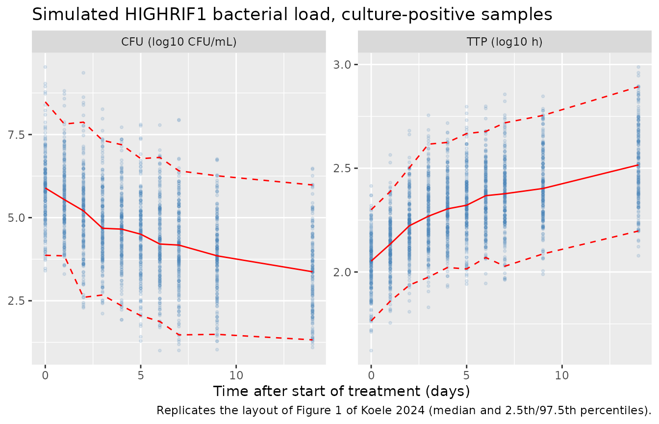
The percentiles read off Figure 1 (the centres of the authors’ simulated prediction intervals) are compared with the simulation below. TTP agrees within about 0.05 log10 h. For CFU the simulated median runs 0.1-0.25 log10 CFU/mL below the authors’ band, and from Day 7 on the simulated 97.5th percentile runs about 0.3-0.7 below it (0.3-0.5 in a 5000-subject run, so not only sampling noise); see ‘Assumptions and deviations’.
fig1 <- tibble::tribble(
  ~endpoint,            ~day, ~fig1_p50, ~fig1_p975,
  "CFU (log10 CFU/mL)",  0,   6.1,       8.2,
  "CFU (log10 CFU/mL)",  7,   4.4,       7.1,
  "CFU (log10 CFU/mL)", 14,   3.5,       6.5,
  "TTP (log10 h)",       0,   2.00,      2.34,
  "TTP (log10 h)",       7,   2.35,      2.68,
  "TTP (log10 h)",      14,   2.50,      2.85
)
fig1 |>
  dplyr::left_join(vpc_rif, by = c("endpoint", "day")) |>
  dplyr::select(endpoint, day, fig1_p50, p50, fig1_p975, p975) |>
  dplyr::rename(
    "Endpoint" = endpoint, "Day" = day,
    "Median, Figure 1" = fig1_p50, "Median, simulated" = p50,
    "97.5th, Figure 1" = fig1_p975, "97.5th, simulated" = p975
  ) |>
knitr::kable(digits = 2, caption = "Figure 1 prediction-interval centres (digitised) vs this simulation, culture-positive samples.")| Endpoint | Day | Median, Figure 1 | Median, simulated | 97.5th, Figure 1 | 97.5th, simulated |
|---|---|---|---|---|---|
| CFU (log10 CFU/mL) | 0 | 6.10 | 5.89 | 8.20 | 8.48 |
| CFU (log10 CFU/mL) | 7 | 4.40 | 4.17 | 7.10 | 6.41 |
| CFU (log10 CFU/mL) | 14 | 3.50 | 3.37 | 6.50 | 5.98 |
| TTP (log10 h) | 0 | 2.00 | 2.05 | 2.34 | 2.30 |
| TTP (log10 h) | 7 | 2.35 | 2.38 | 2.68 | 2.72 |
| TTP (log10 h) | 14 | 2.50 | 2.52 | 2.85 | 2.89 |
The culture-negative proportions are not affected by prediction correction, so they are the sharper check of the residual-error and censoring structure. Figure 1 shows roughly 5% of CFU samples negative on Day 0 rising to about 22% on Day 14, and TTP rising from 0% to about 5%.
neg_tab <- vpc_rif |>
  dplyr::select(endpoint, day, prop_negative) |>
  tidyr::pivot_wider(names_from = endpoint, values_from = prop_negative)
knitr::kable(neg_tab, digits = 3, caption = "Simulated proportion of culture-negative samples by day (Figure 1 lower panels).")| day | CFU (log10 CFU/mL) | TTP (log10 h) |
|---|---|---|
| 0 | 0.050 | 0.000 |
| 1 | 0.035 | 0.000 |
| 2 | 0.060 | 0.000 |
| 3 | 0.055 | 0.000 |
| 4 | 0.080 | 0.000 |
| 5 | 0.060 | 0.005 |
| 6 | 0.075 | 0.000 |
| 7 | 0.065 | 0.000 |
| 9 | 0.100 | 0.000 |
| 14 | 0.235 | 0.035 |
neg_cfu <- vpc_rif |> dplyr::filter(endpoint == "CFU (log10 CFU/mL)")
neg_overall <- sim_rif |> dplyr::group_by(endpoint) |> dplyr::summarise(prop = mean(negative))
knitr::kable(neg_overall, digits = 3, caption = "Overall simulated culture-negative proportion; observed 7.7% (CFU) and 1.1% (TTP).")| endpoint | prop |
|---|---|
| CFU (log10 CFU/mL) | 0.082 |
| TTP (log10 h) | 0.004 |
stopifnot(
  # Day 14: Figure 1 shows about 22% (prediction band ~15-30%). With 200
  # subjects the simulated proportion has a standard error of ~3%.
  abs(neg_cfu$prop_negative[neg_cfu$day == 14] - 0.22) < 0.10,
  # Days 0-7 sit near the 6.4% baseline chance in both Figure 1 and here.
  abs(median(neg_cfu$prop_negative[neg_cfu$day <= 7]) - 0.064) < 0.04
)
Residual-error scale
Table 2 prints the additive errors as 0.334 (CFU) and 0.00667 (TTP) with log10 units, which reads like standard deviations. They are encoded as variances (SD = 0.578 and 0.0817). The Day-0 width of Figure 1’s 95% prediction interval separates the two readings, because at Day 0 only the baseline variability and the residual error contribute. The intervals digitised from Figure 1 are 3.74-8.17 log10 CFU/mL (width 4.43) and 1.80-2.34 log10 h (width 0.53).
set.seed(1)
day0_width <- function(e0, cv, resid_sd, n = 1e5) {
  y <- e0 * exp(stats::rnorm(n, 0, sqrt(log(1 + cv^2)))) + stats::rnorm(n, 0, resid_sd)
  unname(diff(quantile(y, c(0.025, 0.975))))
}
widths <- data.frame(
  endpoint = c("CFU", "TTP"),
  figure1 = c(4.43, 0.53),
  variance_reading = c(day0_width(5.92, 0.154, sqrt(0.334)), day0_width(2.02, 0.055, sqrt(0.00667))),
  sd_reading = c(day0_width(5.92, 0.154, 0.334), day0_width(2.02, 0.055, 0.00667))
)
knitr::kable(widths, digits = 3, caption = "Day-0 95% prediction-interval width: Figure 1 vs the two readings of Table 2.")| endpoint | figure1 | variance_reading | sd_reading |
|---|---|---|---|
| CFU | 4.43 | 4.285 | 3.831 |
| TTP | 0.53 | 0.540 | 0.436 |
Part 2 – the hypothetical-drug simulation models
Exposure and dose
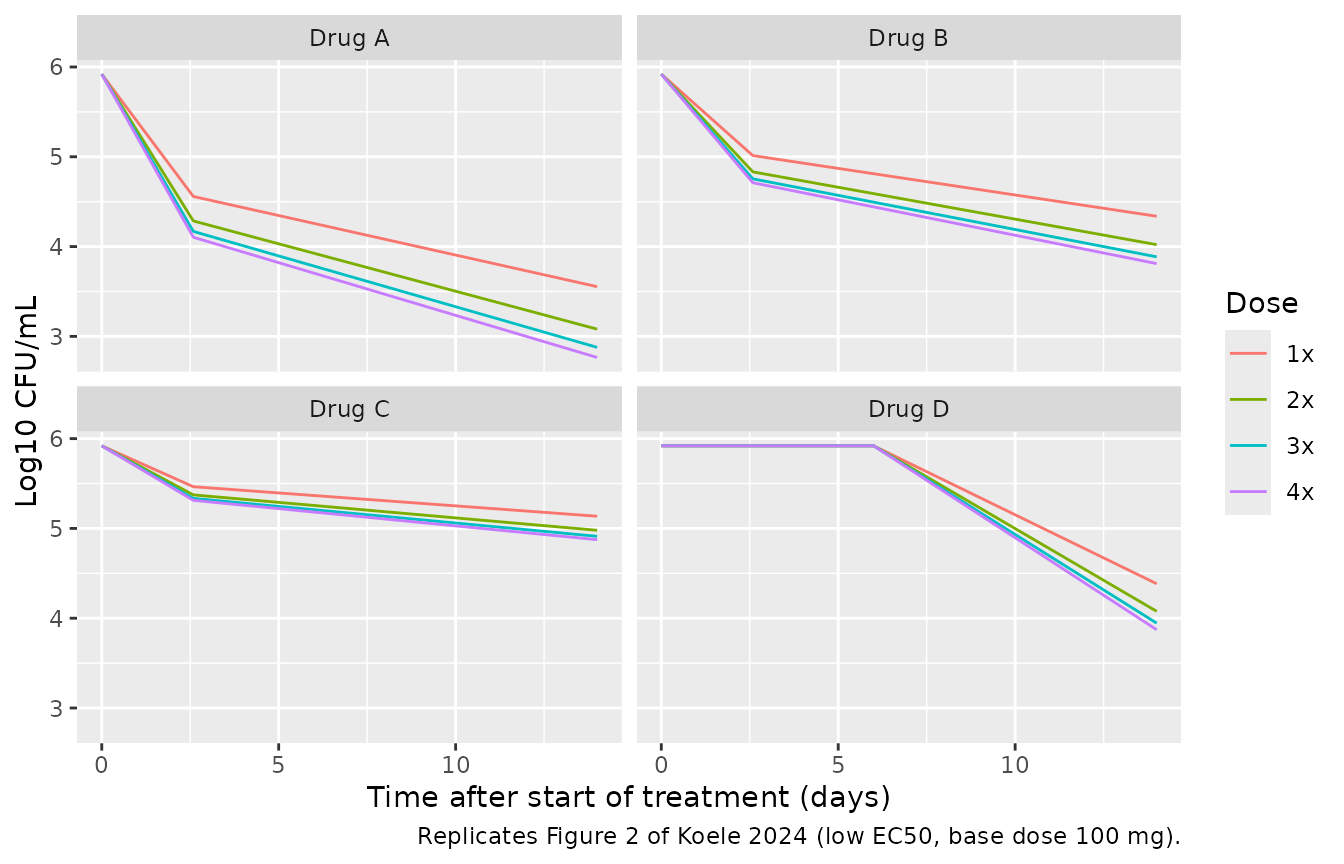
The paper gives the PK constants but not the base daily dose. Each slope depends on the dose only through , and Figure 2 (typical CFU profiles at 1x-4x) pins it: the 1x, 2x and 4x curves for drug A all imply a typical 1x AUC0-24 of 10 mg*h/L, i.e. a base dose of 100 mg at CL = 10 L/h. It is consistent with the Methods, which place the low EC50 (5.0) below the average 1x exposure (10) and the high EC50 (25) below the average 3x exposure (30).
drug_models <- c(
  A = "Koele_2024_TB_drugA", B = "Koele_2024_TB_drugB",
  C = "Koele_2024_TB_drugC", D = "Koele_2024_TB_drugD"
)
base_dose <- 100 # mg; back-solved from Figure 2
dose_levels <- c(`1x` = 1, `2x` = 2, `3x` = 3, `4x` = 4)

make_events <- function(n, multiple, obs_times, id_offset = 0L) {
  ids <- id_offset + seq_len(n)
  dose_rows <- expand.grid(id = ids, time = 24 * (0:13)) |>
    dplyr::mutate(amt = base_dose * multiple, evid = 1L, dvid = NA_integer_)
  obs_rows <- expand.grid(id = ids, time = obs_times) |>
    dplyr::mutate(amt = 0, evid = 0L, dvid = 1L)
  dplyr::bind_rows(dose_rows, obs_rows) |>
    dplyr::mutate(cmt = "central", dose_level = names(dose_levels)[multiple]) |>
    dplyr::arrange(id, time, dplyr::desc(evid))
}
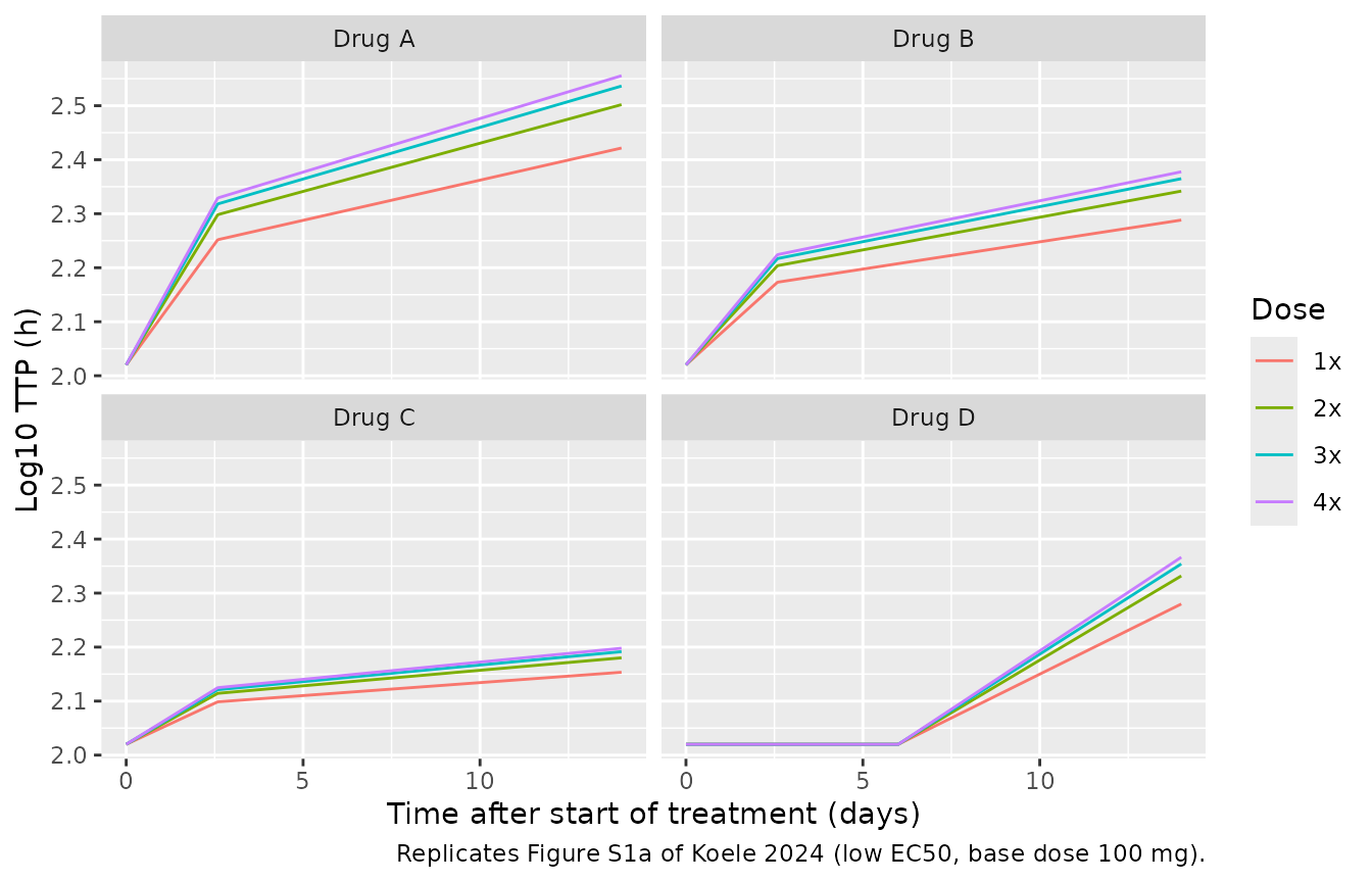
Typical CFU profiles (Figure 2) and TTP profiles (Figure S1a)
typ_events <- dplyr::bind_rows(lapply(seq_along(dose_levels), function(i) {
  make_events(1L, i, obs_times = 0:336, id_offset = i - 1L)
}))
typ_hyp <- dplyr::bind_rows(lapply(names(drug_models), function(d) {
  m <- rxode2::zeroRe(readModelDb(drug_models[[d]]))
  rxode2::rxSolve(m, typ_events, keep = "dose_level", returnType = "data.frame", useLinCmt = FALSE) |>
    dplyr::mutate(drug = paste("Drug", d))
}))
#> ℹ parameter labels from comments will be replaced by 'label()'
#> ℹ omega/sigma items treated as zero: 'etalcl', 'etale0_cfu', 'etale0_ttp', 'etalemax1_cfu', 'etalemax1_ttp', 'etalemax2_cfu', 'etalemax2_ttp'
#> Warning: multi-subject simulation without without 'omega'
#> ℹ parameter labels from comments will be replaced by 'label()'
#> ℹ omega/sigma items treated as zero: 'etalcl', 'etale0_cfu', 'etale0_ttp', 'etalemax1_cfu', 'etalemax1_ttp', 'etalemax2_cfu', 'etalemax2_ttp'
#> Warning: multi-subject simulation without without 'omega'
#> ℹ parameter labels from comments will be replaced by 'label()'
#> ℹ omega/sigma items treated as zero: 'etalcl', 'etale0_cfu', 'etale0_ttp', 'etalemax1_cfu', 'etalemax1_ttp', 'etalemax2_cfu', 'etalemax2_ttp'
#> Warning: multi-subject simulation without without 'omega'
#> ℹ parameter labels from comments will be replaced by 'label()'
#> ℹ omega/sigma items treated as zero: 'etalcl', 'etale0_cfu', 'etale0_ttp', 'etalemax2_cfu', 'etalemax2_ttp'
#> Warning: multi-subject simulation without without 'omega'

ggplot(typ_hyp, aes(time / 24, log_cfu, colour = dose_level)) +
  geom_line() +
  facet_wrap(~drug) +
  labs(
    x = "Time after start of treatment (days)", y = "Log10 CFU/mL", colour = "Dose",
    caption = "Replicates Figure 2 of Koele 2024 (low EC50, base dose 100 mg)."
  )
ggplot(typ_hyp, aes(time / 24, log_ttp, colour = dose_level)) +
  geom_line() +
  facet_wrap(~drug) +
  labs(
    x = "Time after start of treatment (days)", y = "Log10 TTP (h)", colour = "Dose",
    caption = "Replicates Figure S1a of Koele 2024 (low EC50, base dose 100 mg)."
  )
The Day-14 end points of the 16 Figure 2 curves were digitised by the maintainers from the published figure (reading precision about 0.03 log10). The typical-value simulation reproduces all of them.
fig2_day14 <- tibble::tribble(
  ~drug,    ~dose_level, ~fig2,
  "Drug A", "1x", 3.56, "Drug A", "2x", 3.09, "Drug A", "3x", 2.89, "Drug A", "4x", 2.80,
  "Drug B", "1x", 4.34, "Drug B", "2x", 4.05, "Drug B", "3x", 3.92, "Drug B", "4x", 3.83,
  "Drug C", "1x", 5.14, "Drug C", "2x", 4.99, "Drug C", "3x", 4.92, "Drug C", "4x", 4.89,
  "Drug D", "1x", 4.39, "Drug D", "2x", 4.10, "Drug D", "3x", 3.97, "Drug D", "4x", 3.90
)
chk_fig2 <- typ_hyp |>
  dplyr::filter(time == 336) |>
  dplyr::select(drug, dose_level, log_cfu) |>
  dplyr::inner_join(fig2_day14, by = c("drug", "dose_level")) |>
  dplyr::mutate(diff = log_cfu - fig2)
chk_fig2 |>
  dplyr::rename("Drug" = drug, "Dose" = dose_level, "Simulated" = log_cfu, "Figure 2" = fig2, "Difference" = diff) |>
knitr::kable(digits = 3, caption = "Typical log10 CFU/mL on Day 14: simulation vs Figure 2.")| Drug | Dose | Simulated | Figure 2 | Difference |
|---|---|---|---|---|
| Drug A | 1x | 3.554 | 3.56 | -0.006 |
| Drug A | 2x | 3.080 | 3.09 | -0.010 |
| Drug A | 3x | 2.878 | 2.89 | -0.012 |
| Drug A | 4x | 2.765 | 2.80 | -0.035 |
| Drug B | 1x | 4.338 | 4.34 | -0.002 |
| Drug B | 2x | 4.021 | 4.05 | -0.029 |
| Drug B | 3x | 3.886 | 3.92 | -0.034 |
| Drug B | 4x | 3.810 | 3.83 | -0.020 |
| Drug C | 1x | 5.136 | 5.14 | -0.004 |
| Drug C | 2x | 4.979 | 4.99 | -0.011 |
| Drug C | 3x | 4.912 | 4.92 | -0.008 |
| Drug C | 4x | 4.875 | 4.89 | -0.015 |
| Drug D | 1x | 4.384 | 4.39 | -0.006 |
| Drug D | 2x | 4.077 | 4.10 | -0.023 |
| Drug D | 3x | 3.945 | 3.97 | -0.025 |
| Drug D | 4x | 3.872 | 3.90 | -0.028 |
The Methods describe drug A as giving at most a 3 log10 CFU/mL decrease over 14 days, drug B 2, drug C 1, and drug D a maximum similar to drug B. At the highest (4x) dose the typical decreases are:
typ_hyp |>
  dplyr::filter(time == 336, dose_level == "4x") |>
  dplyr::transmute(Drug = drug, `Decrease over 14 days, 4x dose (log10 CFU/mL)` = 5.92 - log_cfu) |>
knitr::kable(digits = 2)| Drug | Decrease over 14 days, 4x dose (log10 CFU/mL) |
|---|---|
| Drug A | 3.16 |
| Drug B | 2.11 |
| Drug C | 1.05 |
| Drug D | 2.05 |
High EC50 scenario (Figures S1b and S1c)
The high-EC50 scenario is the same model with
lec50 = log(25).
typ_high <- dplyr::bind_rows(lapply(names(drug_models), function(d) {
  m <- rxode2::zeroRe(readModelDb(drug_models[[d]])) |> rxode2::ini(lec50 = log(25))
  rxode2::rxSolve(m, typ_events, keep = "dose_level", returnType = "data.frame", useLinCmt = FALSE) |>
    dplyr::mutate(drug = paste("Drug", d))
}))
#> ℹ parameter labels from comments will be replaced by 'label()'
#> ℹ change initial estimate of `lec50` to `3.2188758248682`
#> ℹ omega/sigma items treated as zero: 'etalcl', 'etale0_cfu', 'etale0_ttp', 'etalemax1_cfu', 'etalemax1_ttp', 'etalemax2_cfu', 'etalemax2_ttp'
#> Warning: multi-subject simulation without without 'omega'
#> ℹ parameter labels from comments will be replaced by 'label()'
#> ℹ change initial estimate of `lec50` to `3.2188758248682`
#> ℹ omega/sigma items treated as zero: 'etalcl', 'etale0_cfu', 'etale0_ttp', 'etalemax1_cfu', 'etalemax1_ttp', 'etalemax2_cfu', 'etalemax2_ttp'
#> Warning: multi-subject simulation without without 'omega'
#> ℹ parameter labels from comments will be replaced by 'label()'
#> ℹ change initial estimate of `lec50` to `3.2188758248682`
#> ℹ omega/sigma items treated as zero: 'etalcl', 'etale0_cfu', 'etale0_ttp', 'etalemax1_cfu', 'etalemax1_ttp', 'etalemax2_cfu', 'etalemax2_ttp'
#> Warning: multi-subject simulation without without 'omega'
#> ℹ parameter labels from comments will be replaced by 'label()'
#> ℹ change initial estimate of `lec50` to `3.2188758248682`
#> ℹ omega/sigma items treated as zero: 'etalcl', 'etale0_cfu', 'etale0_ttp', 'etalemax2_cfu', 'etalemax2_ttp'
#> Warning: multi-subject simulation without without 'omega'
typ_high |>
  dplyr::select(drug, dose_level, time, log_cfu, log_ttp) |>
  tidyr::pivot_longer(c(log_cfu, log_ttp), names_to = "endpoint") |>
  ggplot(aes(time / 24, value, colour = dose_level, linetype = drug)) +
  geom_line() +
  facet_wrap(~endpoint, scales = "free_y") +
  labs(
    x = "Time after start of treatment (days)", y = NULL, colour = "Dose", linetype = NULL,
    caption = "Replicates Figures S1b and S1c of Koele 2024 (high EC50)."
  )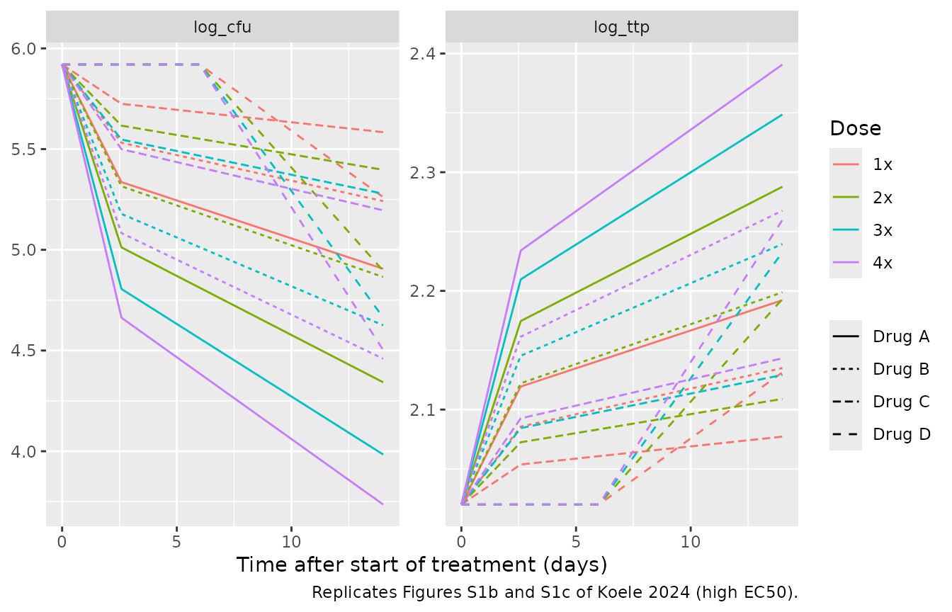
# With EC50 = 25 the 1x dose reaches only 10 / 35 of the maximum slope, so
# the dose levels spread further apart than at the low EC50.
spread <- function(x) {
  d14 <- x |> dplyr::filter(time == 336, drug == "Drug B")
  d14$log_cfu[d14$dose_level == "1x"] - d14$log_cfu[d14$dose_level == "4x"]
}
c(low_ec50 = spread(typ_hyp), high_ec50 = spread(typ_high))
#>  low_ec50 high_ec50
#> 0.5274267 0.7824462
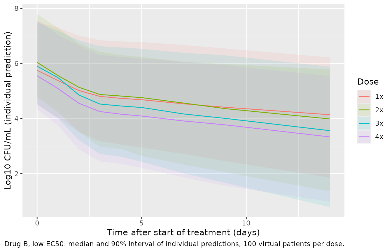
Stochastic simulation, drug B (reference scenario)
Drug B with the low EC50 is the reference for the paper’s design and sensitivity analyses. The clinical trial simulations sampled CFU and TTP on Days 0-5, 7, 9 and 14; a dense grid over the last dosing interval (Days 13-14) is added for the NCA below.
rxode2::rxSetSeed(13089)
n_arm <- 100L
pd_times <- c(0:5, 7, 9, 14) * 24
pk_times <- seq(312, 336, by = 0.5)
ev_b <- dplyr::bind_rows(lapply(seq_along(dose_levels), function(i) {
  make_events(n_arm, i, obs_times = sort(unique(c(pd_times, pk_times))), id_offset = (i - 1L) * n_arm)
}))
stopifnot(!anyDuplicated(unique(ev_b[, c("id", "time", "evid")])))
sim_b <- rxode2::rxSolve(readModelDb("Koele_2024_TB_drugB"), ev_b,
  keep = "dose_level", returnType = "data.frame", useLinCmt = FALSE
)
#> ℹ parameter labels from comments will be replaced by 'label()'

sim_b |>
  dplyr::filter(time %in% pd_times) |>
  dplyr::group_by(dose_level, day = time / 24) |>
  dplyr::summarise(
    p05 = quantile(log_cfu, 0.05), p50 = median(log_cfu), p95 = quantile(log_cfu, 0.95),
    .groups = "drop"
  ) |>
  ggplot(aes(day, p50, colour = dose_level, fill = dose_level)) +
  geom_ribbon(aes(ymin = p05, ymax = p95), alpha = 0.1, colour = NA) +
  geom_line() +
  labs(
    x = "Time after start of treatment (days)", y = "Log10 CFU/mL (individual prediction)",
    colour = "Dose", fill = "Dose",
    caption = "Drug B, low EC50: median and 90% interval of individual predictions, 100 virtual patients per dose."
  )
PKNCA validation of the exposure driver
The bacterial-load slopes are driven by
auc24 = dose / CL, the steady-state AUC0-24 of a
one-compartment model. PKNCA computes the AUC over the last dosing
interval of the simulated concentrations, which must agree with it
subject by subject.
conc_b <- sim_b |>
  dplyr::filter(time >= 312, !is.na(Cc)) |>
  dplyr::select(id, time, Cc, dose_level)
dose_b <- ev_b |>
  dplyr::filter(evid == 1, time == 312) |>
  dplyr::select(id, time, amt, dose_level)

conc_obj <- PKNCA::PKNCAconc(conc_b, Cc ~ time | dose_level + id)
dose_obj <- PKNCA::PKNCAdose(dose_b, amt ~ time | dose_level + id, route = "intravascular")
intervals <- data.frame(start = 312, end = 336, cmax = TRUE, auclast = TRUE)
nca_b <- PKNCA::pk.nca(PKNCA::PKNCAdata(conc_obj, dose_obj, intervals = intervals))

nca_wide <- as.data.frame(nca_b$result) |>
  dplyr::select(id, dose_level, PPTESTCD, PPORRES) |>
  tidyr::pivot_wider(names_from = PPTESTCD, values_from = PPORRES)
auc_model <- sim_b |>
  dplyr::filter(time == 336) |>
  dplyr::select(id, auc24)
chk_auc <- dplyr::inner_join(nca_wide, auc_model, by = "id") |>
  dplyr::mutate(pct_diff = 100 * (auclast - auc24) / auc24)

nca_summary <- chk_auc |>
  dplyr::group_by(dose_level) |>
  dplyr::summarise(
    cmax_median = median(cmax),
    auc_nca_median = median(auclast),
    auc_model_median = median(auc24),
    typical_auc = base_dose * dose_levels[[dose_level[1]]] / 10,
    .groups = "drop"
  )
nca_summary |>
  dplyr::rename(
    "Dose" = dose_level,
    "Cmax, median (mg/L)" = cmax_median,
    "AUC0-24 by PKNCA, median (mg*h/L)" = auc_nca_median,
    "auc24 = dose/CL, median (mg*h/L)" = auc_model_median,
    "Typical dose/CL (mg*h/L)" = typical_auc
  ) |>
knitr::kable(digits = 2, caption = "Day-14 NCA of drug B by dose level (100 virtual patients each).")| Dose | Cmax, median (mg/L) | AUC0-24 by PKNCA, median (mg*h/L) | auc24 = dose/CL, median (mg*h/L) | Typical dose/CL (mg*h/L) |
|---|---|---|---|---|
| 1x | 2.51 | 10.01 | 10.01 | 10 |
| 2x | 5.01 | 19.96 | 19.96 | 20 |
| 3x | 7.52 | 31.27 | 31.27 | 30 |
| 4x | 10.03 | 40.41 | 40.41 | 40 |
stopifnot(
  # Same drawn CL on both sides: only the trapezoid error of the 0.5 h grid
  # separates them.
  abs(median(chk_auc$pct_diff)) < 1,
  quantile(abs(chk_auc$pct_diff), 0.9) < 2,
  # Methods: low EC50 (5.0) below the average 1x exposure, high EC50 (25)
  # below the average 3x exposure.
  nca_summary$auc_nca_median[nca_summary$dose_level == "1x"] > 5,
  nca_summary$auc_nca_median[nca_summary$dose_level == "3x"] > 25
)
Koele 2024 reports no NCA for the hypothetical drugs, so there is no published table to compare against; the check above validates the exposure metric that drives the model.
What is not reproduced
The paper’s main results (Table 3, Figures 3 and 4, Figures S2-S4) are statistical powers from Monte-Carlo mapped power analysis: every simulated trial is re-fitted with the full Emax model and the reduced constant-slope model (Equation 3), and the likelihood-ratio test is evaluated over 10,000 replicates. That needs re-estimation in NONMEM or nlmixr2 and is outside the scope of a validation article. The misspecified linear exposure-response model (Equation 4) is an analysis model only, with no reported estimates, and is not packaged.
Assumptions and deviations
- Residual-error scale. Table 2 prints the additive errors as 0.334 log10 CFU/mL and 0.00667 log10 h. They are treated as $SIGMA variances and encoded as SDs of 0.578 and 0.0817: the Day-0 width of the Figure 1 prediction intervals matches the variance reading (see above), an SD of 0.00667 log10 h would be an implausible 1.5% replicate CV for TTP, and the same group’s BTZ-043 model (Koele 2025, built with the same methods) printed $SIGMA variances of 0.30-0.32 for CFU and 0.0035-0.0043 for TTP.
- Residual correlations not encoded. The model has one residual per endpoint. The correlation between the CFU and TTP additive errors (-47.4%) and the correlations between duplicate-sample replicate errors (CFU 90.3%, TTP 82.7%) are not represented, because nlmixr2lib has no idiomatic residual correlation across outputs or replicates. Marginal distributions are unaffected.
-
Culture-negative likelihood. The M3 handling of
culture-negative samples and the baseline chance of a negative culture
(PBAC = 6.4% CFU, 0.35% TTP) belong to the likelihood, not the
structural model, and are reproduced in this article’s simulation code
rather than in the model files. To fit the models to data with
culture-negative samples, use nlmixr2’s censoring columns
(
CENS,LIMIT). -
IIV form. Equation 2 is printed as
* (1 + IIV), but the Methods (‘Individual baseline bacterial load and slope were assumed to be log-normally distributed’), the Table 2 CV formula and the Supplementary File S1 code (THETA * EXP(ETA)) all use exponential variability, which is what is encoded. - Supplementary File S1 $THETA comments. The $THETA comment labels (EC50 as THETA 7) do not match the $PRED code (EC50 as THETA 5, shared by CFU and TTP). The models follow the $PRED code.
- ULOQ. The control stream sets the TTP ULOQ to 3.003641; log10 of 42 days in hours is 3.003461. The difference is immaterial and the control-stream value is used here.
- Base dose. The base daily dose of the hypothetical drugs is not stated; 100 mg (typical AUC0-24 10 mg*h/L at CL 10 L/h) was back-solved by the maintainers from Figure 2 and reproduces all 16 of its curves.
-
PK route. The PK model is described by CL and V
only. The dose is put into
central; the route does not change AUC0-24, which is all the PD uses. - Drug D node. The Methods describe drug D’s onset as ‘after 7 days’, but Table 2 (node 144 h) and Figure 2d both place it at Day 6; 144 h is used. Drug D has no first-phase slope (Table 2: ‘D: 0’), so its model omits the slope-1 parameters and their variability.
-
Estimation status. The hypothetical-drug PK
constants are wrapped in
fixed()because the authors never estimated them (the analysis model takes AUC0-24 as data). The PD values are left unfixed because the authors re-estimated the PD model on every simulated trial. - pcVPC differences. The TTP percentiles and the culture-negative proportions agree with Figure 1. For CFU, the simulated median sits 0.1-0.25 log10 below the centre of the authors’ median band, and from Day 7 on the simulated 97.5th percentile sits 0.3-0.5 log10 below theirs (5000-subject run), i.e. the authors’ upper CFU tail declines more slowly than the Table 2 variabilities produce here. Prediction correction, the censoring rule applied in the authors’ VPC and the exact sampling times of the baseline samples cannot be reconstructed from the paper, and no reading of Table 2 that changes the slope variabilities is supported by the text, so the parameters are kept as printed and the VPC percentiles are reported but not used as a gate.
- Errata. No correction notice for Koele 2024 was found (Crossref and Europe PMC, checked 2026-10-29).