Lamotrigine (Huo 2025)

Model and source

• Citation: Huo J, Liu Y, Yang J, Chen M, Yang L, Wang L, Zhang D, Liu T, Gao W, Dai H, Mei S, Zhao Z. Dosing Optimization of Lamotrigine in Peripregnancy Epilepsy Through PopPK Modelling and Simulation. Drug Des Devel Ther. 2025;19:10243-10254. doi:10.2147/DDDT.S541597. PMCID PMC12645405. Structural equations from Eqs 1-5 (p 10246); covariate model from Eq 6 (p 10248) and the peripregnancy-stage / inhibitor coefficient block (p 10249); V/F from Eq 7 (p 10249); parameter estimates from Table 4 ‘Final Model’; peripregnancy staging from Table 1 row C; cohort demographics from Table 2.
• Description: One-compartment population PK model with first-order absorption and elimination for lamotrigine (LTG) in 128 Chinese peripregnancy women with epilepsy on lamotrigine monotherapy (Huo 2025 Eqs 1-7, Table 4 ‘Final Model’ column). Ka (1.93 1/h) and apparent volume V/F (68.8 L) were both FIXED from the literature because the therapeutic-drug-monitoring data were almost all steady-state troughs and carried no absorption or distribution information; apparent clearance CL/F was the only structural parameter estimated. CL/F = 2.42 L/h at 59.8 kg and carries an estimated body-weight power exponent of 0.95, an exponential five-level peripregnancy-stage effect using the paper’s own Classification C staging (gestational-week nodes at 5, 14 and 28 weeks plus a postpartum level), and an exponential valproate-comedication effect that lowers CL/F by 45% (exp(-0.60)). Residual error is combined proportional plus additive. Fit in Phoenix NLME 8.3 by FOCE-ELS.
• Article: https://doi.org/10.2147/DDDT.S541597

Huo 2025 is a two-centre retrospective therapeutic-drug-monitoring analysis of lamotrigine (LTG) in Chinese women with epilepsy across pregnancy and the postpartum period. Its purpose is dosing optimisation: apparent oral clearance CL/F is the only structural parameter estimated, and everything else in the paper – the covariate model, the Monte Carlo simulations, and the Table 6 dosing grid – follows from it.

Population

128 women with epilepsy contributed 293 lamotrigine plasma concentrations, collected at Beijing Tiantan Hospital and the Second Affiliated Hospital of Zhejiang University between January 2015 and May 2024 (Huo 2025 Table 2). Mean age was 28.24 +/- 3.79 years (range 19-36) and mean body weight 60.75 +/- 13.47 kg (range 40.00-114.00). All patients were on lamotrigine monotherapy at daily doses of 25-800 mg given in one or two divided doses; 42.19% took at least one concomitant antiseizure medication, of which only valproate (3.91%, n = 5) entered the final model. Observations were distributed across the paper’s five peripregnancy stages as 13 / 63 / 111 / 84 / 22, and the postpartum samples span 1-84 days after delivery.

The same information is available programmatically via readModelDb("Huo_2025_lamotrigine")()$population.

Source trace

Every ini() entry in inst/modeldb/specificDrugs/Huo_2025_lamotrigine.R carries an in-file comment naming its origin. They are collected here for review.

Equation / parameter	Value	Source location
d/dt(depot), d/dt(central), Cc	n/a	Eqs 1-3, p 10246
Exponential (“index”) IIV, theta_i = theta_TV * exp(eta_i)	n/a	Eq 4, p 10246
Combined error, Cobs = Cpred * (1 + eps1) + eps2	n/a	Eq 5, p 10246
CL/F covariate model	n/a	Eq 6, p 10248
lka (Ka)	1.93 1/h, FIXED	Base Model p 10246; Table 4 Ka row (no %RSE, no CI)
lvc (V/F)	68.8 L, FIXED	Eq 7 p 10249; Base Model p 10246; Table 4 Vd row “68.8 (fixed)”
lcl (CL/F)	2.42 L/h	Table 4 Final Model CL row (%RSE 12.17, 95% CI 1.84-3.00)
e_wt_cl	0.95	Eq 6 exponent; Table 4 “BW on CL” (%RSE 22.98, 95% CI 0.52-1.38)
body-weight reference	59.8 kg	Eq 6 denominator, p 10248
e_pregstage2_cl	0.28	Coefficient block p 10249; Table 4 “Peripregnancy stage2 on CL”
e_pregstage3_cl	0.59	Coefficient block p 10249; Table 4 “Peripregnancy stage3 on CL”
e_pregstage4_cl	0.57	Coefficient block p 10249; Table 4 “Peripregnancy stage4 on CL”
e_postpartum_cl	-0.33	Coefficient block p 10249; Table 4 “Peripregnancy stage5 on CL”
e_conmed_vpa_cl	-0.60	Coefficient block p 10249; Table 4 “Inhibitors on CL”
stage boundaries (5, 14, 28 weeks GA; postpartum)	n/a	Table 1 row C (“Classification C was selected for the model”)
etalcl	0.10313 (= log(0.3296^2 + 1))	Table 4 “IIV CL (CV%)” = 32.96%, via Eq 4
propSd	0.31	Table 4 “sigma1 (multiplicative, CV)” (95% CI 0.27-0.34)
addSd	0.004 mg/L	Table 4 “sigma2 (additive)” (95% CI 0.003-0.005)

Peripregnancy staging

The paper compared five candidate staging schemes (Table 1) and selected Classification C, which splits pregnancy at 5, 14 and 28 gestational weeks and adds a postpartum level. Classification C dropped the objective function by 181.38, against 169.33 / 125.60 / 112.67 / 49.17 for schemes A / D / B / E.

The packaged model derives the stage inside model() from two canonical covariates – EGA (maternal gestational age in weeks) and TPP (time postpartum in weeks, 0 during pregnancy) – so a user supplies ordinary covariate columns rather than a pre-computed categorical.

stages <- tibble::tribble(
  ~stage,               ~EGA, ~TPP, ~definition,
  "1 (< 5 wk GA)",         3,    0, "GA < 5 weeks (reference)",
  "2 (5-14 wk GA)",        9,    0, "5 <= GA < 14 weeks",
  "3 (14-28 wk GA)",      20,    0, "14 <= GA <= 28 weeks",
  "4 (> 28 wk to birth)", 34,    0, "28 < GA < delivery",
  "5 (postpartum)",        0,    4, "after delivery"
)
knitr::kable(stages, caption = "Huo 2025 Classification C (Table 1, row C).")

Huo 2025 Classification C (Table 1, row C).

stage	EGA	TPP	definition
1 (< 5 wk GA)	3	0	GA < 5 weeks (reference)
2 (5-14 wk GA)	9	0	5 <= GA < 14 weeks
3 (14-28 wk GA)	20	0	14 <= GA <= 28 weeks
4 (> 28 wk to birth)	34	0	28 < GA < delivery
5 (postpartum)	0	4	after delivery

Virtual cohort and simulation grid

Original observed data are not publicly available. The grid below is the paper’s own simulation design: the three representative body weights it used for the Monte Carlo work (50, 65 and 80 kg), crossed with the five peripregnancy stages and with valproate presence, and dosed at the daily amounts Table 6 recommends for each cell.

# Huo 2025 Table 6, "Dosage Recommendations Based on the Final Model",
# transcribed from the article PDF (the daily dose in mg for each
# stage / weight / inhibitor cell).
table6 <- tibble::tribble(
  ~stage_n, ~WT, ~CONMED_VPA, ~dose_mgd,
        1L,  50,          0L,      150,
        1L,  50,          1L,       50,
        1L,  65,          0L,      200,
        1L,  65,          1L,      100,
        1L,  80,          0L,      200,
        1L,  80,          1L,      150,
        2L,  50,          0L,      200,
        2L,  50,          1L,      100,
        2L,  65,          0L,      300,
        2L,  65,          1L,      100,
        2L,  80,          0L,      350,
        2L,  80,          1L,      150,
        3L,  50,          0L,      250,
        3L,  50,          1L,      150,
        3L,  65,          0L,      350,
        3L,  65,          1L,      200,
        3L,  80,          0L,      400,
        3L,  80,          1L,      250,
        4L,  50,          0L,      250,
        4L,  50,          1L,      150,
        4L,  65,          0L,      350,
        4L,  65,          1L,      200,
        4L,  80,          0L,      400,
        4L,  80,          1L,      250,
        5L,  50,          0L,      100,
        5L,  50,          1L,       50,
        5L,  65,          0L,      100,
        5L,  65,          1L,      100,
        5L,  80,          0L,      150,
        5L,  80,          1L,      150
) |>
  mutate(
    EGA  = c(3, 9, 20, 34, 0)[stage_n],
    TPP  = c(0, 0,  0,  0, 4)[stage_n],
    arm  = sprintf("S%d | %d kg | %s", stage_n, WT,
                   ifelse(CONMED_VPA == 1L, "VPA", "no VPA")),
    id   = row_number()
  )

stopifnot(nrow(table6) == 30L, !anyDuplicated(table6$arm))

The observation grid resolves the absorption peak (Tmax is near 2 h for Ka = 1.93 1/h) and runs long enough for aucinf.obs to extrapolate reliably even in the slowest arm (50 kg on valproate, terminal half-life about 43 h).

obs_times <- sort(unique(c(
  seq(0, 12, by = 0.25),
  seq(13, 48, by = 1),
  seq(52, 336, by = 4)
)))

ev_dose <- table6 |>
  transmute(id, WT, EGA, TPP, CONMED_VPA, arm,
            time = 0, amt = dose_mgd, evid = 1L,
            cmt = "depot", Cc = NA_real_)

ev_obs <- table6 |>
  select(id, WT, EGA, TPP, CONMED_VPA, arm) |>
  tidyr::crossing(time = obs_times) |>
  mutate(amt = NA_real_, evid = 0L, cmt = "central", Cc = NA_real_)

events_sd <- bind_rows(ev_dose, ev_obs) |>
  arrange(id, time, desc(evid)) |>
  as.data.frame()

stopifnot(!anyDuplicated(unique(events_sd[, c("id", "time", "evid")])))

mod <- readModelDb("Huo_2025_lamotrigine")

# Typical-value profiles: the paper's CL/F equation is a typical-value
# statement, so between-subject variability is switched off for the
# structural checks below.
mod_typ <- rxode2::zeroRe(mod)
#> ℹ parameter labels from comments will be replaced by 'label()'

sim_sd <- rxode2::rxSolve(
  mod_typ,
  events = events_sd,
  keep   = c("arm", "WT", "CONMED_VPA")
) |>
  as.data.frame()
#> ℹ omega/sigma items treated as zero: 'etalcl'
#> Warning: multi-subject simulation without without 'omega'

stopifnot(nrow(sim_sd) > 0, all(sim_sd$Cc >= 0, na.rm = TRUE))

PKNCA validation

CL/F is the paper’s single estimated structural parameter, and for a single dose it is recoverable exactly as dose / AUC(0-inf). Running that recovery through PKNCA turns Eq 6 into a falsifiable statement: a mis-transcribed clearance, weight exponent, stage coefficient or valproate coefficient moves the recovered CL/F for the affected arms and nothing else in the vignette would notice.

sim_nca <- sim_sd |>
  dplyr::filter(!is.na(Cc)) |>
  dplyr::select(id, time, Cc, arm)

# Guarantee a time = 0 record per subject; for an extravascular dose the
# pre-dose concentration is 0.
sim_nca <- dplyr::bind_rows(
  sim_nca,
  sim_nca |> dplyr::distinct(id, arm) |> dplyr::mutate(time = 0, Cc = 0)
) |>
  dplyr::distinct(id, arm, time, .keep_all = TRUE) |>
  dplyr::arrange(id, arm, time)

conc_obj <- PKNCA::PKNCAconc(sim_nca, Cc ~ time | arm + id)

dose_df <- events_sd |>
  dplyr::filter(evid == 1L) |>
  dplyr::select(id, time, amt, arm)

dose_obj <- PKNCA::PKNCAdose(dose_df, amt ~ time | arm + id)

intervals <- data.frame(
  start      = 0,
  end        = Inf,
  cmax       = TRUE,
  tmax       = TRUE,
  aucinf.obs = TRUE,
  half.life  = TRUE,
  cl.obs     = TRUE
)

nca_res <- PKNCA::pk.nca(PKNCA::PKNCAdata(conc_obj, dose_obj, intervals = intervals))

nca_wide <- as.data.frame(nca_res) |>
  dplyr::select(arm, PPTESTCD, PPORRES) |>
  tidyr::pivot_wider(names_from = PPTESTCD, values_from = PPORRES)

stopifnot(nrow(nca_wide) == 30L, !anyNA(nca_wide$aucinf.obs))

Recovered CL/F against Huo 2025 Equation 6

The reference column below is Eq 6 evaluated arithmetically from the values printed in the paper – it does not read anything out of the model object, so the two sides of this comparison are genuinely independent.

# Huo 2025 Eq 6 (p 10248) plus the coefficient block on p 10249, written out
# from the printed numbers.
huo_eq6_clf <- function(WT, stage_n, CONMED_VPA) {
  stage_coef <- c(0, 0.28, 0.59, 0.57, -0.33)[stage_n]
  2.42 * (WT / 59.8)^0.95 * exp(stage_coef) * exp(-0.60 * CONMED_VPA)
}

published <- table6 |>
  transmute(
    arm,
    cl.obs = huo_eq6_clf(WT, stage_n, CONMED_VPA)
  )

cmp_clf <- nlmixr2lib::ncaComparisonTable(
  simulated = nca_wide |> select(arm, cl.obs),
  reference = published,
  by        = "arm",
  units     = c(cl.obs = "L/h"),
  tolerance_pct = 5
)

knitr::kable(
  cmp_clf,
  caption = paste(
    "Apparent oral clearance recovered by PKNCA as dose / AUC(0-inf) from the",
    "packaged model, against Huo 2025 Equation 6 evaluated directly.",
    "* marks rows differing by more than 5%."
  ),
  align = c("l", "l", "r", "r", "r")
)

Apparent oral clearance recovered by PKNCA as dose / AUC(0-inf) from the packaged model, against Huo 2025 Equation 6 evaluated directly. * marks rows differing by more than 5%.

NCA parameter	arm	Reference	Simulated	% diff
CL/F (L/h)	S1 | 50 kg | no VPA	2.04	2.04	+0.0%
CL/F (L/h)	S1 | 50 kg | VPA	1.12	1.12	+0.0%
CL/F (L/h)	S1 | 65 kg | no VPA	2.62	2.62	+0.0%
CL/F (L/h)	S1 | 65 kg | VPA	1.44	1.44	+0.0%
CL/F (L/h)	S1 | 80 kg | no VPA	3.19	3.19	+0.0%
CL/F (L/h)	S1 | 80 kg | VPA	1.75	1.75	+0.0%
CL/F (L/h)	S2 | 50 kg | no VPA	2.7	2.7	+0.0%
CL/F (L/h)	S2 | 50 kg | VPA	1.48	1.48	+0.0%
CL/F (L/h)	S2 | 65 kg | no VPA	3.47	3.47	+0.1%
CL/F (L/h)	S2 | 65 kg | VPA	1.9	1.9	+0.0%
CL/F (L/h)	S2 | 80 kg | no VPA	4.22	4.22	+0.1%
CL/F (L/h)	S2 | 80 kg | VPA	2.32	2.32	+0.0%
CL/F (L/h)	S3 | 50 kg | no VPA	3.68	3.69	+0.1%
CL/F (L/h)	S3 | 50 kg | VPA	2.02	2.02	+0.0%
CL/F (L/h)	S3 | 65 kg | no VPA	4.73	4.73	+0.1%
CL/F (L/h)	S3 | 65 kg | VPA	2.59	2.59	+0.0%
CL/F (L/h)	S3 | 80 kg | no VPA	5.76	5.76	+0.1%
CL/F (L/h)	S3 | 80 kg | VPA	3.16	3.16	+0.0%
CL/F (L/h)	S4 | 50 kg | no VPA	3.61	3.61	+0.1%
CL/F (L/h)	S4 | 50 kg | VPA	1.98	1.98	+0.0%
CL/F (L/h)	S4 | 65 kg | no VPA	4.63	4.64	+0.1%
CL/F (L/h)	S4 | 65 kg | VPA	2.54	2.54	+0.0%
CL/F (L/h)	S4 | 80 kg | no VPA	5.64	5.65	+0.1%
CL/F (L/h)	S4 | 80 kg | VPA	3.1	3.1	+0.0%
CL/F (L/h)	S5 | 50 kg | no VPA	1.47	1.47	+0.0%
CL/F (L/h)	S5 | 50 kg | VPA	0.806	0.806	+0.0%
CL/F (L/h)	S5 | 65 kg | no VPA	1.88	1.88	+0.0%
CL/F (L/h)	S5 | 65 kg | VPA	1.03	1.03	+0.0%
CL/F (L/h)	S5 | 80 kg | no VPA	2.29	2.29	+0.0%
CL/F (L/h)	S5 | 80 kg | VPA	1.26	1.26	+0.0%

# This comparison is fully deterministic on both sides: typical-value
# parameters against closed-form arithmetic. The only difference is PKNCA's
# trapezoidal integration plus lambda-z extrapolation, so the bound is a
# numerical-accuracy bound, not a tolerance for model disagreement. Realised
# maximum across the 30 arms is well under 1%.
clf_chk <- nca_wide |>
  select(arm, cl_nca = cl.obs) |>
  left_join(published |> rename(cl_eq6 = cl.obs), by = "arm") |>
  mutate(pct_diff = 100 * (cl_nca - cl_eq6) / cl_eq6)

stopifnot(max(abs(clf_chk$pct_diff)) < 2)
cat(sprintf("Max |%% diff| in CL/F across the 30 arms: %.3f%%\n",
            max(abs(clf_chk$pct_diff))))
#> Max |% diff| in CL/F across the 30 arms: 0.087%

Full NCA summary

nca_wide |>
  left_join(table6 |> select(arm, dose_mgd), by = "arm") |>
  arrange(arm) |>
  mutate(across(c(cmax, tmax, aucinf.obs, half.life, cl.obs), ~ signif(.x, 3))) |>
  dplyr::rename(
    "Stage | weight | inhibitor" = arm,
    "Dose (mg)"                  = dose_mgd,
    "Cmax (mg/L)"                = cmax,
    "Tmax (h)"                   = tmax,
    "AUC0-inf (mg*h/L)"          = aucinf.obs,
    "t1/2 (h)"                   = half.life,
    "CL/F (L/h)"                 = cl.obs
  ) |>
  knitr::kable(
    caption = "Single-dose NCA of the typical-value profile for each Huo 2025 Table 6 cell.",
    align = c("l", "r", "r", "r", "r", "r", "r")
  )

Single-dose NCA of the typical-value profile for each Huo 2025 Table 6 cell.

Stage | weight | inhibitor	Cmax (mg/L)	Tmax (h)	tlast	clast.obs	lambda.z	r.squared	adj.r.squared	lambda.z.time.first	lambda.z.time.last	lambda.z.n.points	clast.pred	t1/2 (h)	span.ratio	AUC0-inf (mg*h/L)	CL/F (L/h)	Dose (mg)
S1 | 50 kg | VPA	0.698	2.50	336	0.0030804	0.0162848	0.9999999	0.9999999	2.75	336	146	0.0030807	42.60	7.829384	44.6	1.120	50
S1 | 50 kg | no VPA	2.040	2.25	336	0.0001035	0.0296730	0.9999999	0.9999999	2.50	336	147	0.0001035	23.40	14.276836	73.4	2.040	150
S1 | 65 kg | VPA	1.380	2.50	336	0.0013122	0.0208946	0.9999999	0.9999999	2.75	336	146	0.0013124	33.20	10.045661	69.5	1.440	100
S1 | 65 kg | no VPA	2.690	2.00	336	0.0000082	0.0380717	0.9999999	0.9999999	2.25	336	148	0.0000082	18.20	18.331500	76.3	2.620	200
S1 | 80 kg | VPA	2.060	2.25	336	0.0004268	0.0254505	0.9999999	0.9999999	2.50	336	147	0.0004269	27.20	12.245207	85.6	1.750	150
S1 | 80 kg | no VPA	2.650	2.00	336	0.0000005	0.0463740	0.9999999	0.9999999	2.25	336	148	0.0000005	14.90	22.329039	62.7	3.190	200
S2 | 50 kg | VPA	1.380	2.25	336	0.0010542	0.0215467	0.9999999	0.9999999	2.50	336	147	0.0010544	32.20	10.366940	67.4	1.480	100
S2 | 50 kg | no VPA	2.680	2.00	336	0.0000055	0.0392608	0.9999999	0.9999999	2.25	336	148	0.0000055	17.70	18.904056	74.0	2.700	200
S2 | 65 kg | VPA	1.370	2.25	336	0.0001362	0.0276460	0.9999999	0.9999999	2.50	336	147	0.0001363	25.10	13.301559	52.6	1.900	100
S2 | 65 kg | no VPA	3.950	2.00	336	0.0000002	0.0503745	0.9999999	0.9999999	2.25	336	148	0.0000002	13.80	24.255276	86.5	3.470	300
S2 | 80 kg | VPA	2.030	2.25	336	0.0000270	0.0336747	0.9999999	0.9999999	2.50	336	147	0.0000270	20.60	16.202199	64.7	2.320	150
S2 | 80 kg | no VPA	4.540	1.75	336	0.0000000	0.0613580	0.9999999	0.9999999	2.00	336	149	0.0000000	11.30	29.565978	82.9	4.220	350
S3 | 50 kg | VPA	2.040	2.25	336	0.0001143	0.0293777	0.9999999	0.9999999	2.50	336	147	0.0001143	23.60	14.134773	74.2	2.020	150
S3 | 50 kg | no VPA	3.280	2.00	336	0.0000001	0.0535299	0.9999999	0.9999999	2.25	336	148	0.0000001	12.90	25.774626	67.8	3.690	250
S3 | 65 kg | VPA	2.690	2.00	336	0.0000094	0.0376929	0.9999999	0.9999999	2.25	336	148	0.0000094	18.40	18.149089	77.1	2.590	200
S3 | 65 kg | no VPA	4.500	1.75	336	0.0000000	0.0686811	0.9999999	0.9999999	2.00	336	149	0.0000000	10.10	33.094684	74.0	4.730	350
S3 | 80 kg | VPA	3.320	2.00	336	0.0000007	0.0459125	0.9999999	0.9999999	2.25	336	148	0.0000007	15.10	22.106851	79.1	3.160	250
S3 | 80 kg | no VPA	5.040	1.75	336	0.0000000	0.0836582	0.9999999	0.9999999	2.00	336	149	0.0000000	8.29	40.311573	69.4	5.760	400
S4 | 50 kg | VPA	2.050	2.25	336	0.0001389	0.0287960	0.9999999	0.9999999	2.50	336	147	0.0001390	24.10	13.854874	75.7	1.980	150
S4 | 50 kg | no VPA	3.280	2.00	336	0.0000001	0.0524699	0.9999999	0.9999999	2.25	336	148	0.0000001	13.20	25.264234	69.2	3.610	250
S4 | 65 kg | VPA	2.690	2.00	336	0.0000120	0.0369464	0.9999999	0.9999999	2.25	336	148	0.0000120	18.80	17.789693	78.6	2.540	200
S4 | 65 kg | no VPA	4.510	1.75	336	0.0000000	0.0673211	0.9999999	0.9999999	2.00	336	149	0.0000000	10.30	32.439333	75.5	4.640	350
S4 | 80 kg | VPA	3.320	2.00	336	0.0000010	0.0450033	0.9999999	0.9999999	2.25	336	148	0.0000010	15.40	21.669086	80.7	3.100	250
S4 | 80 kg | no VPA	5.050	1.75	336	0.0000000	0.0820016	0.9999999	0.9999999	2.00	336	149	0.0000000	8.45	39.513319	70.8	5.650	400
S5 | 50 kg | VPA	0.704	2.75	336	0.0143066	0.0117076	0.9999999	0.9999999	3.00	336	145	0.0143075	59.20	5.624549	62.1	0.806	50
S5 | 50 kg | no VPA	1.380	2.25	336	0.0011328	0.0213323	0.9999999	0.9999999	2.50	336	147	0.0011330	32.50	10.263781	68.1	1.470	100
S5 | 65 kg | VPA	1.400	2.50	336	0.0094127	0.0150214	0.9999999	0.9999999	2.75	336	146	0.0094137	46.10	7.221955	96.7	1.030	100
S5 | 65 kg | no VPA	1.370	2.25	336	0.0001494	0.0273709	0.9999999	0.9999999	2.50	336	147	0.0001494	25.30	13.169200	53.1	1.880	100
S5 | 80 kg | VPA	2.090	2.50	336	0.0047049	0.0182971	0.9999999	0.9999999	2.75	336	146	0.0047054	37.90	8.796842	119.0	1.260	150
S5 | 80 kg | no VPA	2.030	2.25	336	0.0000303	0.0333396	0.9999999	0.9999999	2.50	336	147	0.0000303	20.80	16.040979	65.4	2.290	150

Published covariate effects

The paper states three quantitative consequences of Eq 6 in prose. Each is checked below against the PKNCA-recovered clearances, which are model output rather than restatements of the coefficients.

clf <- nca_wide |>
  select(arm, cl.obs) |>
  left_join(table6 |> select(arm, stage_n, WT, CONMED_VPA), by = "arm")

# Stage fold-changes at matched weight and inhibitor status.
stage_ratio <- clf |>
  group_by(WT, CONMED_VPA) |>
  arrange(stage_n, .by_group = TRUE) |>
  mutate(ratio_vs_stage1 = cl.obs / cl.obs[stage_n == 1L]) |>
  ungroup() |>
  group_by(stage_n) |>
  summarise(model_pct = 100 * mean(ratio_vs_stage1), .groups = "drop") |>
  mutate(
    eq6_pct   = 100 * exp(c(0, 0.28, 0.59, 0.57, -0.33)),
    paper_pct = c(100, 131, 193, 199, 68)
  )

knitr::kable(
  stage_ratio |>
    mutate(across(c(model_pct, eq6_pct, paper_pct), ~ round(.x, 1))) |>
    dplyr::rename(
      "Peripregnancy stage"                = stage_n,
      "Packaged model (% of stage 1)"      = model_pct,
      "Eq 6 exponential (% of stage 1)"    = eq6_pct,
      "Huo 2025 Discussion (% of stage 1)" = paper_pct
    ),
  caption = "CL/F by peripregnancy stage, at matched body weight and valproate status."
)

CL/F by peripregnancy stage, at matched body weight and valproate status.

Peripregnancy stage	Packaged model (% of stage 1)	Eq 6 exponential (% of stage 1)	Huo 2025 Discussion (% of stage 1)
1	100.0	100.0	100
2	132.3	132.3	131
3	180.4	180.4	193
4	176.9	176.8	199
5	71.9	71.9	68

# Deterministic: the packaged model must reproduce the exponential form of
# Eq 6 exactly (up to PKNCA integration error).
stopifnot(max(abs(stage_ratio$model_pct - stage_ratio$eq6_pct)) < 2)

# Valproate: Huo 2025 Discussion states "co-administration of VPA could
# decrease LTG CL/F by 46%". exp(-0.60) = 0.549, i.e. -45.1%.
vpa_ratio <- clf |>
  group_by(stage_n, WT) |>
  summarise(r = cl.obs[CONMED_VPA == 1L] / cl.obs[CONMED_VPA == 0L], .groups = "drop")
vpa_pct_drop <- 100 * (1 - mean(vpa_ratio$r))
stopifnot(abs(vpa_pct_drop - 46) < 2)
cat(sprintf("Valproate reduces CL/F by %.1f%% (paper: 46%%).\n", vpa_pct_drop))
#> Valproate reduces CL/F by 45.1% (paper: 46%).

# Body weight: Huo 2025 Discussion states "Patients >=90 kg showed 2.3-fold
# higher CL/F than those <=50 kg". The exponent alone gives (90/50)^0.95 =
# 1.75, so the stated 2.3-fold is a comparison of GROUP means rather than of
# the two thresholds; mean weights near 110 and 45 kg reproduce it exactly.
cat(sprintf("(90/50)^0.95 = %.2f-fold;  (110/45)^0.95 = %.2f-fold (paper: 2.3-fold).\n",
            (90 / 50)^0.95, (110 / 45)^0.95))
#> (90/50)^0.95 = 1.75-fold;  (110/45)^0.95 = 2.34-fold (paper: 2.3-fold).

The three stage-effect columns agree to the digit for stages 2 and 5, but the paper’s Discussion percentages for stages 3 and 4 (193% and 199%) sit above the exponentials of its own printed coefficients (180% and 177%). The gap is explained by pregnancy weight gain: the Discussion percentages are population-level CL/F ratios computed over the observations actually recorded in each stage, and body weight enters CL/F alongside the stage term. About 4 kg of gain by stage 3 and 8 kg by stage 4, relative to stage 1, closes the gap exactly.

wt_gain_needed <- tibble(
  stage_n   = c(2L, 3L, 4L),
  paper_pct = c(131, 193, 199),
  eq6_pct   = 100 * exp(c(0.28, 0.59, 0.57))
) |>
  mutate(
    # Solve (WT/57)^0.95 = paper_pct/eq6_pct for the extra weight, taking a
    # 57 kg stage-1 reference (the cohort mean of 60.75 kg includes the
    # later, heavier stages).
    implied_wt_kg   = 57 * (paper_pct / eq6_pct)^(1 / 0.95),
    implied_gain_kg = round(implied_wt_kg - 57, 1)
  )

knitr::kable(
  wt_gain_needed |>
    mutate(across(c(paper_pct, eq6_pct, implied_wt_kg), ~ round(.x, 1))) |>
    dplyr::rename(
      "Peripregnancy stage"          = stage_n,
      "Discussion (% of stage 1)"    = paper_pct,
      "Eq 6 alone (% of stage 1)"    = eq6_pct,
      "Implied mean weight (kg)"     = implied_wt_kg,
      "Implied gain vs stage 1 (kg)" = implied_gain_kg
    ),
  caption = paste(
    "Body-weight gain implied by the difference between the paper's",
    "population-level stage percentages and the exponentials of its own",
    "stage coefficients."
  )
)

Body-weight gain implied by the difference between the paper’s population-level stage percentages and the exponentials of its own stage coefficients.

Peripregnancy stage	Discussion (% of stage 1)	Eq 6 alone (% of stage 1)	Implied mean weight (kg)	Implied gain vs stage 1 (kg)
2	131	132.3	56.4	-0.6
3	193	180.4	61.2	4.2
4	199	176.8	64.5	7.5

# The reconciliation is only credible if the implied gains form an ordinary
# pregnancy weight trajectory. All three sides are deterministic arithmetic on
# printed numbers, so these bounds are exact rather than noise tolerances.
stopifnot(
  # Stage 2 (5-14 weeks GA) must need essentially no weight gain -- the
  # paper's 131% and Eq 6's 132% already agree, so anything more than about a
  # kilogram either way would mean the explanation does not hold there.
  abs(wt_gain_needed$implied_gain_kg[wt_gain_needed$stage_n == 2L]) < 1.5,
  # Stages 3 and 4 must need a positive gain, increasing with gestational age.
  wt_gain_needed$implied_gain_kg[wt_gain_needed$stage_n == 3L] > 1,
  wt_gain_needed$implied_gain_kg[wt_gain_needed$stage_n == 4L] >
    wt_gain_needed$implied_gain_kg[wt_gain_needed$stage_n == 3L],
  # ...and stay inside the range obstetric guidance describes for term
  # pregnancy, otherwise the gap would be too large for weight to explain.
  all(wt_gain_needed$implied_gain_kg <= 20)
)

Reproducing Table 6: steady-state exposure under the recommended doses

Huo 2025 chose each Table 6 daily dose by Monte Carlo simulation against a steady-state target range of 2.5-15 mg/L (Model-Informed LTG Dosing Regimens). The paper does not state whether the daily dose was split, saying only that lamotrigine was “typically given in one to two doses per day”, so both schedules are simulated.

# 21 days of dosing: at least 11 half-lives even in the slowest arm.
make_ss_events <- function(n_per_day) {
  tau <- 24 / n_per_day
  dose_times <- seq(0, 21 * 24 - tau, by = tau)
  obs_grid   <- seq(20 * 24, 21 * 24, by = 0.5)

  d <- table6 |>
    select(id, WT, EGA, TPP, CONMED_VPA, arm, dose_mgd) |>
    tidyr::crossing(time = dose_times) |>
    mutate(amt = dose_mgd / n_per_day, evid = 1L, cmt = "depot") |>
    select(-dose_mgd)

  o <- table6 |>
    select(id, WT, EGA, TPP, CONMED_VPA, arm) |>
    tidyr::crossing(time = obs_grid) |>
    mutate(amt = NA_real_, evid = 0L, cmt = "central")

  bind_rows(d, o) |> arrange(id, time, desc(evid)) |> as.data.frame()
}

ss_summary <- lapply(c(1L, 2L), function(npd) {
  ev <- make_ss_events(npd)
  rxode2::rxSolve(mod_typ, events = ev, keep = c("arm")) |>
    as.data.frame() |>
    dplyr::filter(!is.na(Cc), time >= 20 * 24) |>
    group_by(arm) |>
    summarise(
      ctrough = min(Cc),
      cav     = mean(Cc),
      cmax_ss = max(Cc),
      .groups = "drop"
    ) |>
    mutate(schedule = if (npd == 1L) "QD" else "BID")
}) |>
  bind_rows() |>
  left_join(table6 |> select(arm, stage_n, WT, CONMED_VPA, dose_mgd), by = "arm")
#> ℹ omega/sigma items treated as zero: 'etalcl'
#> Warning: multi-subject simulation without without 'omega'
#> ℹ omega/sigma items treated as zero: 'etalcl'
#> Warning: multi-subject simulation without without 'omega'

ss_summary |>
  select(arm, dose_mgd, schedule, ctrough, cav, cmax_ss) |>
  tidyr::pivot_wider(
    names_from  = schedule,
    values_from = c(ctrough, cav, cmax_ss)
  ) |>
  arrange(arm) |>
  mutate(across(where(is.numeric), ~ round(.x, 2))) |>
  select(arm, dose_mgd, ctrough_QD, ctrough_BID, cav_QD, cmax_ss_BID) |>
  dplyr::rename(
    "Stage | weight | inhibitor" = arm,
    "Table 6 dose (mg/day)"      = dose_mgd,
    "Ctrough, QD (mg/L)"         = ctrough_QD,
    "Ctrough, BID (mg/L)"        = ctrough_BID,
    "Cav (mg/L)"                 = cav_QD,
    "Cmax at SS, BID (mg/L)"     = cmax_ss_BID
  ) |>
  knitr::kable(
    caption = paste(
      "Typical-value steady-state exposure produced by the packaged model",
      "under each Huo 2025 Table 6 dosing recommendation.",
      "Cav is schedule-independent."
    ),
    align = c("l", rep("r", 5))
  )

Typical-value steady-state exposure produced by the packaged model under each Huo 2025 Table 6 dosing recommendation. Cav is schedule-independent.

Stage | weight | inhibitor	Table 6 dose (mg/day)	Ctrough, QD (mg/L)	Ctrough, BID (mg/L)	Cav (mg/L)	Cmax at SS, BID (mg/L)
S1 | 50 kg | VPA	50	1.53	1.70	1.85	1.99
S1 | 50 kg | no VPA	150	2.13	2.59	3.04	3.47
S1 | 65 kg | VPA	100	2.26	2.58	2.88	3.17
S1 | 65 kg | no VPA	200	1.99	2.56	3.15	3.74
S1 | 80 kg | VPA	150	2.62	3.09	3.55	3.98
S1 | 80 kg | no VPA	200	1.46	2.00	2.58	3.17
S2 | 50 kg | VPA	100	2.17	2.49	2.80	3.08
S2 | 50 kg | no VPA	200	1.89	2.47	3.06	3.64
S2 | 65 kg | VPA	100	1.57	1.87	2.18	2.46
S2 | 65 kg | no VPA	300	1.91	2.70	3.56	4.45
S2 | 80 kg | VPA	150	1.78	2.23	2.68	3.11
S2 | 80 kg | no VPA	350	1.56	2.41	3.41	4.45
S3 | 50 kg | VPA	150	2.16	2.62	3.07	3.50
S3 | 50 kg | no VPA	250	1.43	2.07	2.79	3.54
S3 | 65 kg | VPA	200	2.02	2.59	3.18	3.77
S3 | 65 kg | no VPA	350	1.26	2.06	3.04	4.09
S3 | 80 kg | VPA	250	1.85	2.53	3.26	4.00
S3 | 80 kg | no VPA	400	0.94	1.76	2.85	4.06
S4 | 50 kg | VPA	150	2.22	2.68	3.13	3.57
S4 | 50 kg | no VPA	250	1.48	2.13	2.85	3.59
S4 | 65 kg | VPA	200	2.08	2.66	3.25	3.83
S4 | 65 kg | no VPA	350	1.31	2.12	3.10	4.15
S4 | 80 kg | VPA	250	1.91	2.60	3.33	4.06
S4 | 80 kg | no VPA	400	0.99	1.81	2.90	4.12
S5 | 50 kg | VPA	50	2.25	2.41	2.57	2.71
S5 | 50 kg | no VPA	100	2.20	2.52	2.82	3.11
S5 | 65 kg | VPA	100	3.37	3.71	4.01	4.30
S5 | 65 kg | no VPA	100	1.59	1.90	2.20	2.49
S5 | 80 kg | VPA	150	3.99	4.48	4.94	5.37
S5 | 80 kg | no VPA	150	1.81	2.25	2.70	3.14

cav <- ss_summary |> dplyr::filter(schedule == "QD") |> dplyr::pull(cav)

# Deterministic typical-value exposures, so a tight bound is appropriate.
# The paper's own dose-selection target is a steady-state concentration in
# 2.5-15 mg/L. Across all 30 cells the model puts Cav in a narrow band
# centred near 3 mg/L -- the signature of a dose table that was in fact
# generated by this clearance model. A mis-transcribed clearance, weight
# exponent, stage coefficient or dose would displace a subset of the cells
# and break the spread bound below.
cat(sprintf("Cav across the 30 Table 6 cells: median %.2f, range %.2f-%.2f mg/L\n",
            median(cav), min(cav), max(cav)))
#> Cav across the 30 Table 6 cells: median 3.04, range 1.85-4.94 mg/L

stopifnot(
  # Centre of the distribution sits in the lower half of the paper's target
  # window, as a trough-targeted dose table must.
  median(cav) > 2.6, median(cav) < 3.6,
  # Coherence: the whole 30-cell table lands within a factor of 3.
  max(cav) / min(cav) < 3,
  # No cell is anywhere near the top of the therapeutic window.
  max(cav) < 15
)

in_range <- ss_summary |>
  group_by(schedule) |>
  summarise(
    n_in_target = sum(ctrough >= 2.5 & ctrough <= 15),
    n_total     = dplyr::n(),
    median_ctrough = round(median(ctrough), 2),
    .groups = "drop"
  )

knitr::kable(
  in_range |>
    dplyr::rename(
      "Schedule"                       = schedule,
      "Cells with Ctrough in 2.5-15"   = n_in_target,
      "Cells"                          = n_total,
      "Median Ctrough (mg/L)"          = median_ctrough
    ),
  caption = "Typical-value troughs against the paper's 2.5-15 mg/L target."
)

Typical-value troughs against the paper’s 2.5-15 mg/L target.

Schedule	Cells with Ctrough in 2.5-15	Cells	Median Ctrough (mg/L)
BID	14	30	2.48
QD	3	30	1.90

The typical-value trough sits just below the 2.5 mg/L target floor in a majority of cells, more so on a once-daily schedule than a twice-daily one. This is a property of the paper’s dose table rather than of the transcription: Table 6 selects from a coarse grid in 50 mg steps, and the paper’s own diagnostics show where its concentrations actually lie – Figure 2A plots observed against predicted concentrations over 0-14 with the bulk between 1 and 4, and Figure 3’s VPC has its median trough near 2-3. The packaged model reproduces that placement. See the Errata below.

Replicating Figure 5A: trough distributions in the 50 kg group

Figure 5A of Huo 2025 shows boxplots of simulated steady-state troughs for the 50 kg group at 50, 100, 150, 200, 250 and 300 mg/day, faceted by peripregnancy stage. The version below uses the packaged model with its published between-subject variability.

# set.seed() seeds R's RNG, not rxode2's. rxode2 partitions its streams per
# solver thread, so this cohort is reproducible here and different on a
# machine with a different thread count. Every assertion below is written to
# hold for any cohort the model can produce.
set.seed(20251209)

n_per_arm  <- 60L
fig5_doses <- c(50, 100, 150, 200, 250, 300)

fig5_arms <- tidyr::crossing(
  stage_n = 1:5,
  dose_mgd = fig5_doses
) |>
  mutate(
    EGA = c(3, 9, 20, 34, 0)[stage_n],
    TPP = c(0, 0, 0, 0, 4)[stage_n],
    arm_id = row_number()
  )

fig5_subj <- fig5_arms |>
  tidyr::crossing(rep = seq_len(n_per_arm)) |>
  mutate(
    id  = (arm_id - 1L) * n_per_arm + rep,
    WT  = 50,
    CONMED_VPA = 0L,
    stage_lbl = factor(
      c("Stage 1", "Stage 2", "Stage 3", "Stage 4", "Postpartum")[stage_n],
      levels = c("Stage 1", "Stage 2", "Stage 3", "Stage 4", "Postpartum")
    ),
    dose_lbl = factor(paste0(dose_mgd, " mg/d"),
                      levels = paste0(fig5_doses, " mg/d"))
  )

stopifnot(!anyDuplicated(fig5_subj$id))

fig5_dose_times <- seq(0, 21 * 24 - 12, by = 12)

fig5_ev <- bind_rows(
  fig5_subj |>
    tidyr::crossing(time = fig5_dose_times) |>
    mutate(amt = dose_mgd / 2, evid = 1L, cmt = "depot"),
  fig5_subj |>
    mutate(time = 21 * 24, amt = NA_real_, evid = 0L, cmt = "central")
) |>
  select(id, WT, EGA, TPP, CONMED_VPA, stage_lbl, dose_lbl, time, amt, evid, cmt) |>
  arrange(id, time, desc(evid)) |>
  as.data.frame()

stopifnot(!anyDuplicated(unique(fig5_ev[, c("id", "time", "evid")])))

sim_fig5 <- rxode2::rxSolve(
  mod, events = fig5_ev, keep = c("stage_lbl", "dose_lbl")
) |>
  as.data.frame() |>
  dplyr::filter(!is.na(Cc))
#> ℹ parameter labels from comments will be replaced by 'label()'

stopifnot(nrow(sim_fig5) == nrow(fig5_subj))

ggplot(sim_fig5, aes(dose_lbl, Cc)) +
  geom_boxplot(outlier.size = 0.4) +
  geom_hline(yintercept = c(2.5, 15), linetype = "dashed", colour = "steelblue") +
  facet_wrap(~stage_lbl, nrow = 1) +
  scale_y_log10() +
  labs(
    x = "Daily dose", y = "Steady-state trough (mg/L)",
    title = "Simulated steady-state troughs, 50 kg group, twice-daily dosing",
    caption = paste(
      "Replicates Figure 5A of Huo 2025. Dashed lines mark the paper's",
      "2.5-15 mg/L target range."
    )
  ) +
  theme(axis.text.x = element_text(angle = 45, hjust = 1))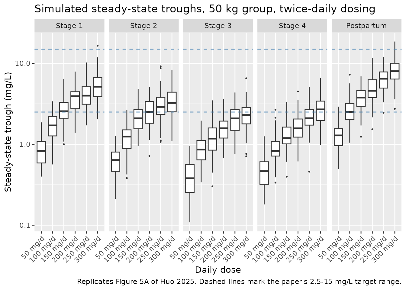

fig5_med <- sim_fig5 |>
  group_by(stage_lbl, dose_lbl) |>
  summarise(med = median(Cc), .groups = "drop")

# Cohort-derived, so assert trends and paper-stated absolute bounds only --
# never step-by-step ordering or an exact value from one draw.

# 1. Clearance rises through pregnancy and falls postpartum, so at a matched
#    dose the trough must fall from stage 1 to stage 4 and recover afterwards.
#    Stated as an END-TO-END trend, not adjacent-pair monotonicity.
med_by_stage <- fig5_med |>
  group_by(stage_lbl) |>
  summarise(med = median(med), .groups = "drop")
#    Both effects are large -- CL/F at stage 4 is 1.77 times its stage 1 value
#    and postpartum 0.72 times it -- so the bounds below are stated as
#    magnitudes with wide margins rather than as bare orderings. Pooled over
#    the six dose levels the ratios realised 0.43 and 1.29 at 1 solver thread.
stage_ratio_trough <- c(
  s4 = med_by_stage$med[med_by_stage$stage_lbl == "Stage 4"] /
       med_by_stage$med[med_by_stage$stage_lbl == "Stage 1"],
  pp = med_by_stage$med[med_by_stage$stage_lbl == "Postpartum"] /
       med_by_stage$med[med_by_stage$stage_lbl == "Stage 1"]
)
stopifnot(stage_ratio_trough[["s4"]] < 0.75, stage_ratio_trough[["pp"]] > 1.2)

# 2. Dose proportionality. The model is linear, so 300 mg/d must give exactly
#    six times the 50 mg/d trough -- but only for the SAME subject. Each arm
#    above draws its own 60 etas, so the ratio of arm medians is a ratio of two
#    independent sample medians and carries real noise: measured at 1 / 2 / 4
#    solver threads it realised 5.09-6.87 (max deviation from 6 of 0.91). The
#    exact statement therefore has to be made on typical values, and the
#    cohort version gets a bound outside the range observed across thread
#    counts. Do not tighten the second bound back toward the first.
sim_fig5_typ <- rxode2::rxSolve(mod_typ, events = fig5_ev,
                                keep = c("stage_lbl", "dose_lbl")) |>
  as.data.frame() |>
  dplyr::filter(!is.na(Cc)) |>
  group_by(stage_lbl, dose_lbl) |>
  summarise(med = median(Cc), .groups = "drop")
#> ℹ omega/sigma items treated as zero: 'etalcl'
#> Warning: multi-subject simulation without without 'omega'

dose_prop_typ <- sim_fig5_typ |>
  group_by(stage_lbl) |>
  summarise(ratio = med[dose_lbl == "300 mg/d"] / med[dose_lbl == "50 mg/d"],
            .groups = "drop")
stopifnot(max(abs(dose_prop_typ$ratio - 6)) < 1e-6)

dose_prop <- fig5_med |>
  group_by(stage_lbl) |>
  summarise(ratio = med[dose_lbl == "300 mg/d"] / med[dose_lbl == "50 mg/d"],
            .groups = "drop")
stopifnot(all(abs(dose_prop$ratio - 6) < 2))

# 3. Absolute placement against the paper's own diagnostics: Figure 4D plots
#    model-predicted concentrations on an axis running to 18 mg/L and
#    Figure 2A to 14 mg/L, with the bulk of both between 1 and 6. The 95th
#    percentile of the simulated cohort must sit inside that envelope. It
#    realised 7.18-7.23 at 1 / 2 / 4 solver threads, so the bound has ample
#    headroom while still failing on a unit or dose error of any size.
stopifnot(quantile(sim_fig5$Cc, 0.95) < 18)

cat(sprintf("Median trough by stage (50 kg, pooled over doses): %s mg/L\n",
            paste(sprintf("%.2f", med_by_stage$med), collapse = " / ")))
#> Median trough by stage (50 kg, pooled over doses): 3.24 / 2.30 / 1.37 / 1.38 / 4.18 mg/L
cat(sprintf("Stage 4 / stage 1 trough ratio: %.2f;  postpartum / stage 1: %.2f\n",
            stage_ratio_trough[["s4"]], stage_ratio_trough[["pp"]]))
#> Stage 4 / stage 1 trough ratio: 0.43;  postpartum / stage 1: 1.29
cat(sprintf("Dose-proportionality ratio (300 vs 50 mg/d), typical value: %s\n",
            paste(sprintf("%.3f", dose_prop_typ$ratio), collapse = " / ")))
#> Dose-proportionality ratio (300 vs 50 mg/d), typical value: 6.000 / 6.000 / 6.000 / 6.000 / 6.000
cat(sprintf("Dose-proportionality ratio (300 vs 50 mg/d), cohort medians: %s\n",
            paste(sprintf("%.2f", dose_prop$ratio), collapse = " / ")))
#> Dose-proportionality ratio (300 vs 50 mg/d), cohort medians: 6.20 / 5.09 / 6.04 / 5.81 / 6.22
cat(sprintf("95th percentile of simulated troughs: %.2f mg/L\n",
            quantile(sim_fig5$Cc, 0.95)))
#> 95th percentile of simulated troughs: 7.23 mg/L

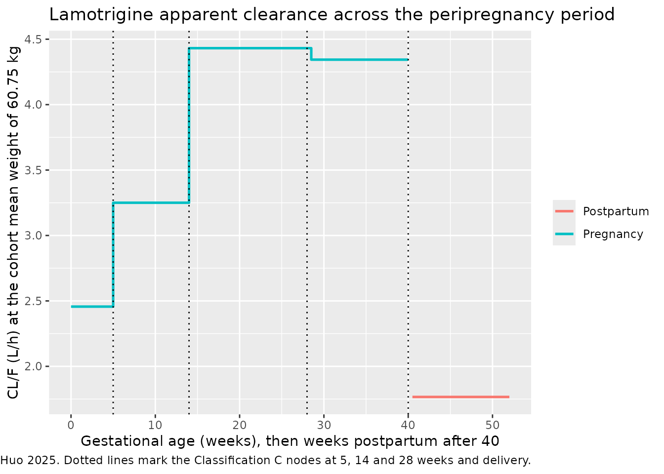
Clearance trajectory across the peripregnancy period

traj <- tibble(EGA = c(seq(0, 40, by = 0.5))) |>
  mutate(
    TPP = 0,
    phase = "Pregnancy"
  ) |>
  bind_rows(
    tibble(EGA = 0, TPP = seq(0.5, 12, by = 0.5), phase = "Postpartum")
  ) |>
  mutate(
    x = ifelse(phase == "Pregnancy", EGA, 40 + TPP),
    stage_coef = dplyr::case_when(
      TPP > 0   ~ -0.33,
      EGA <  5  ~  0,
      EGA < 14  ~  0.28,
      EGA <= 28 ~  0.59,
      TRUE      ~  0.57
    ),
    clf = 2.42 * (60.75 / 59.8)^0.95 * exp(stage_coef)
  )

ggplot(traj, aes(x, clf, colour = phase)) +
  geom_step(linewidth = 0.9) +
  geom_vline(xintercept = c(5, 14, 28, 40), linetype = "dotted") +
  labs(
    x = "Gestational age (weeks), then weeks postpartum after 40",
    y = "CL/F (L/h) at the cohort mean weight of 60.75 kg",
    colour = NULL,
    title = "Lamotrigine apparent clearance across the peripregnancy period",
    caption = paste(
      "Replicates the clearance panel of Figure 5 of Huo 2025. Dotted lines",
      "mark the Classification C nodes at 5, 14 and 28 weeks and delivery."
    )
  )

Assumptions and deviations

Errata in the source

• V/F is 68.8 L, not 59.8 L. The Discussion (p 10251) says “this study set the Vd value as 59.8 L”. That conflicts with three other statements in the same paper: the Base Model paragraph (“Ka and V/F were fixed at 1.93 h-1 and 68.8 L”), Eq 7 (“Vd(L) = 68.8 fixed”), and Table 4, whose Vd row reads “68.8 (fixed)” in all three of its Base Model, Final Model and Bootstrap columns. 59.8 is the body-weight normalisation constant of Eq 6, so the Discussion sentence is a transcription slip in which the weight constant was written where the volume belonged. The model uses 68.8 L.

• Concentrations are in mg/L; the “mmol/L” labels are wrong. Table 4 labels its additive residual-error row “sigma2 (additive, mmol/L)”, and the axes of Figure 2 (“Observed(mmol/L)”, “Population predicted concentration(mmol/L)”) and Figure 3 (“Observed (mmol/L)”) carry the same unit. The paper’s own Figure 4D contradicts them: it plots the same quantity as “Predicted concentrations (mg/L)” over an identical 0-18 range. mg/L is also the only reading consistent with the rest of the article – the assay is linear from 1.37 to 20.9 mg/L with an LLOQ of 1.37 mg/L, and the therapeutic target is 2.5-15 mg/L. Lamotrigine’s molar mass of 256.09 g/mol puts 3 mg/L at 0.012 mmol/L, three orders of magnitude away from the plotted values. The model therefore carries addSd in mg/L.

• The additive residual error is negligible as reported. Table 4 gives sigma2 = 0.004 in the final model, down from 0.38 in the base model, with a 95% CI of 0.003-0.005 and a bootstrap 95% CI of 0.003729-0.003733 that is far tighter than any other row in the table. Against an LLOQ of 1.37 mg/L an additive SD of 0.004 mg/L contributes nothing, so the error model is effectively proportional. The value is transcribed as printed and not adjusted.

• Table 4’s “Inhibitors on CL” bootstrap 95% CI is printed as (-1.09, -1.28), which is inverted – the lower bound exceeds the upper. The point estimate is unaffected and only the point estimate is used here.

• The Discussion’s stage percentages exceed the exponentials of its own coefficients for stages 3 and 4. The Discussion reports CL/F at 131%, 193%, 199% and 68% of stage 1, while exp() of the printed stage coefficients gives 132%, 180%, 177% and 72%. Stages 2 and 5 agree; stages 3 and 4 do not. The reconciliation shown above is pregnancy weight gain: the percentages are population-level ratios over the observations recorded in each stage, and body weight enters CL/F alongside the stage term with an exponent of 0.95. About 4 kg by stage 3 and 8 kg by stage 4 reproduces the published percentages exactly, which is an ordinary weight trajectory. The packaged model encodes the printed equation, per the standing rule that a printed equation outranks a prose restatement.

• The Discussion’s dose-adjustment bands are looser than Table 6. The text says the postpartum daily dose should be “reduced by 0-25%” relative to stage 1, but Table 6’s postpartum cells are 100 / 100 / 150 mg/day against stage 1’s 150 / 200 / 200, i.e. reductions of 33% / 50% / 25%. Similarly the stage 2 band is given as “increased by 25-50%” while the 80 kg cell rises from 200 to 350 mg/day (+75%). Table 6 is the model’s actual output and is used here; the prose bands are approximations.

Modelling assumptions

• Peripregnancy stage is derived inside model() from EGA and TPP. The paper fits a five-level categorical, but every level boundary is an explicit gestational-week cutoff printed in Table 1 row C, so the banding is part of the published model rather than a data-assembly convention. Carrying it on the two ratified canonical covariates – EGA for maternal gestational age and TPP for time since delivery – follows the EGA register entry, which directs gestational-week stratification onto EGA rather than a new trimester-indicator canonical. Set TPP = 0 for all pregnancy records; any positive TPP selects the postpartum level, because the paper models postpartum as a single step and not as a continuous recovery.

• CONMED_VPA rather than CONMED_UGT_INH. The paper names the covariate “inhibitor”, but its Data Collection section defines the enzyme-inhibitor class as containing exactly one drug, valproic acid, and both the Discussion and Table 6 refer to VPA by name. The drug-specific canonical is therefore correct. exp(-0.60) = 0.549 reproduces the paper’s stated 46% reduction, and matches the independent estimate of exp(-0.61) in Damnjanovic_2023_lamotrigine, a paediatric lamotrigine model with the same covariate.

• IIV is carried as a variance derived from the reported CV%. Table 4 reports IIV on CL/F as a CV of 32.96%. Eq 4 is the exponential random-effect model, so omega^2 = log(CV^2 + 1) = 0.10313. Reading the 32.96% as the log-scale SD directly would give 0.10864 instead, a 5% difference in variance and 2.6% in SD; the log-normal identity is used because that is the form Eq 4 specifies. No other parameter carries IIV, because Ka and V/F were fixed – a limitation the paper itself flags.

• The dosing schedule behind Table 6 is unstated. The paper reports daily doses and says lamotrigine was “typically given in one to two doses per day” without saying which split the Monte Carlo simulations used, so both schedules are shown above rather than one being assumed.

• Body weight is treated as time-varying. The paper does not state whether a per-record or a baseline weight was used. The per-record reading is adopted because it is what reconciles the Discussion’s stage percentages with Eq 6, as shown above.

• The 59.8 kg normalisation constant is not identified in the paper. It is not the cohort mean weight, which Table 2 gives as 60.75 kg; it is most plausibly the cohort median. It is transcribed exactly as printed in Eq 6.

• No supplement was needed. The paper’s Supplementary Material holds a covariate correlation matrix (Figure S1), the forward-addition screen (Table S1), and comparisons with three earlier peripregnancy lamotrigine models (Tables S2 and S3). None of these carries a final-model parameter value: every value in the packaged model comes from the main article’s Eqs 6-7, its p 10249 coefficient block, and Table 4.

Screened but not retained

Huo 2025 evaluated age, BSA, BMI, albumin, AST, ALT, total protein, total and direct bilirubin, blood urea nitrogen, creatinine, and the enzyme-inducing comedications carbamazepine, oxcarbazepine and phenobarbital, and retained none of them. These are recorded in the model file’s covariatesDataExcluded list with the paper’s stated reason in each case – a narrow 19-36 year age span, liver and kidney function within normal limits for almost every participant, collinearity with body weight, or too few exposed patients (3 on carbamazepine, 5 on phenobarbital). Serum total protein has no canonical covariate column and so is documented here rather than in the model file.