Perioperative factor VIII (Hazendonk 2016)
Source:vignettes/articles/Hazendonk_2016_factor_viii.Rmd
Hazendonk_2016_factor_viii.RmdModel and source
- Citation: Hazendonk H, Fijnvandraat K, Lock J, Driessens M, van der Meer F, Meijer K, Kruip M, Laros-van Gorkom B, Peters M, de Wildt S, Leebeek F, Cnossen M, Mathot R; OPTI-CLOT study group. A population pharmacokinetic model for perioperative dosing of factor VIII in hemophilia A patients. Haematologica. 2016 Oct;101(10):1159-1169. doi:[10.3324/haematol.2015.136275](https://doi.org/10.3324/haematol.2015.136275). PMID:27390359.
- Description: Two-compartment population PK model for FVIII concentrates in severe and moderate hemophilia A patients (adults and children, FVIII plasma concentration less than 0.05 IU/mL) undergoing elective, minor or major surgery. PK parameters are allometrically scaled to a 68 kg reference body weight with fixed exponents of 0.75 on clearances and 1.0 on volumes. Clearance carries three covariate effects (age with power exponent -0.17 centered at 40 years; +26% for blood group O; -7% for major surgery) and central volume carries an age effect (exponent -0.09). B-domain-deleted recombinant FVIII products (Refacto AF) are under-detected by the one-stage clotting assay by 34%, encoded as a multiplicative correction on the predicted concentration.
- Modality: various registered FVIII concentrates – recombinant products (Kogenate FS, Helixate FS, Advate, Recombinate; also the B-domain-deleted moroctocog Refacto AF) and plasma-derived products (Aafact, Hemofil M). FVIII activity is read out in IU/mL by one-stage clotting assay.
The structural model is a two-compartment IV system with allometric body-weight scaling; the observed quantity is plasma FVIII activity (Hazendonk 2016 Structural model development, Table 5):
with blood_group = 1 for ABO group O (0 otherwise) and
severity = 1 for a major surgical procedure (0 for minor).
The predicted plasma concentration is multiplied by
(1 - theta_bdp * FORM_FVIII_BDD) with
theta_bdp = 0.34 to account for the
one-stage-clotting-assay under-detection of B-domain-deleted FVIII
(Refacto AF).
Population
The derivation cohort consisted of 119 hemophilia A patients (75 adults, 44 children; essentially all-male by X-linked recessive inheritance) undergoing 198 surgical procedures at five Academic Hemophilia Treatment Centers in the Netherlands between 2000 and 2013 (Hazendonk 2016 Table 2). Adults had a median age of 48 years (range 19-78) and a median body weight of 80 kg (45-111 kg); children had a median age of 4.3 years (0.2-17.3) and a median weight of 18.5 kg (5-85 kg). 70% of the cohort had severe hemophilia A (FVIII plasma concentration less than 0.01 IU/mL) and 71% were on long-term prophylaxis. Blood group O was present in about half of the cohort with recorded blood group (50%, 51 of 101 with a value; 34/68 adults, 17/33 children). Major or high-risk surgical procedures accounted for 49% of the 198 procedures (61% of adult procedures, 19% of pediatric procedures); orthopedic surgery was the single most common category (48%), reflecting the adult burden of hemophilic arthropathy.
Perioperative replacement therapy followed the Dutch National Hemophilia Consensus: a pre-operative bolus of about 50 IU/kg FVIII followed by either continuous infusion (58% of procedures) or intermittent bolus (42%), targeting FVIII plasma concentration 0.80-1.00 IU/mL during the first 24 h, 0.50-0.80 IU/mL over 24-120 h, and 0.30-0.50 IU/mL after 120 h. In total the analysis included 1389 FVIII plasma concentration measurements (trough, peak, and steady-state samples), all measured by one-stage clotting assay. Recombinant concentrates accounted for 77% of procedures, of which 14% used the B-domain-deleted moroctocog product Refacto AF; the remaining 23% used plasma-derived FVIII.
The same metadata is available programmatically via the model’s
population element
(readModelDb("Hazendonk_2016_factor_viii")()$population).
Source trace
The per-parameter origin is recorded as an in-file comment next to
each ini() entry in
inst/modeldb/specificDrugs/Hazendonk_2016_factor_viii.R.
The table below collects them in one place.
| Model parameter / equation | Value | Source location |
|---|---|---|
lcl (CL, L/h) |
log(0.150) | Hazendonk 2016 Table 4, “Final model” column: CL = 150 mL/h/68 kg (RSE 8%) |
lvc (V1, L) |
log(2.810) | Hazendonk 2016 Table 4: V1 = 2810 mL/68 kg (RSE 4%) |
lq (Q, L/h) |
log(0.160) | Hazendonk 2016 Table 4: Q = 160 mL/h/68 kg (RSE 20%) |
lvp (V2, L) |
log(1.900) | Hazendonk 2016 Table 4: V2 = 1900 mL/68 kg (RSE 11%) |
theta_bdp (BDP fractional under-prediction) |
0.34 | Hazendonk 2016 Table 4: theta B-domain deleted product = 0.34 (RSE 13%) |
e_age_cl (power on CL) |
-0.17 | Hazendonk 2016 Table 4: theta5 CL-Age = -0.17 (RSE 22%) |
e_age_vc (power on V1) |
-0.09 | Hazendonk 2016 Table 4: theta8 V1-Age = -0.09 (RSE 28%) |
e_blood_cl (linear on CL) |
0.26 | Hazendonk 2016 Table 4: theta6 CL-Blood group O = 26% (RSE 7%) |
e_surg_cl (linear on CL) |
-0.07 | Hazendonk 2016 Table 4: theta7 CL-Major surgery = -7% (RSE 6%) |
allo_cl (fixed exponent on CL, Q) |
0.75 | Hazendonk 2016 Structural model development: “power exponents fixed at 0.75 for clearances” |
allo_vc (fixed exponent on V1, V2) |
1.00 | Hazendonk 2016 Structural model development: “1.0 for volumes of distribution” |
IIV etalcl
|
omega^2 = 0.37^2 = 0.1369 | Hazendonk 2016 Table 4: IIV CL = 37% (RSE 14%) |
IIV etalvc
|
omega^2 = 0.27^2 = 0.0729 | Hazendonk 2016 Table 4: IIV V1 = 27% (RSE 14%) |
addSd (additive RUV, IU/mL) |
0.15 | Hazendonk 2016 Table 4: Centers 1, 2, 3 additive = 0.15 IU/mL (RSE 12%) |
propSd (proportional RUV) |
0.18 | Hazendonk 2016 Table 4: Centers 1, 2, 3 proportional = 0.18 (RSE 15%) |
| Reference body weight | 68 kg | Hazendonk 2016 Structural model development, Table 4 header, Table 5 |
| Reference age (centering) | 40 years | Hazendonk 2016 Table 5 (age/40 in both CL and V1 covariate terms) |
| ODE structure (2-compartment IV) | n/a | Hazendonk 2016 Structural model development, Table 3 model 2 |
| B-domain-deleted correction on observed Cc | Cc = (central/vc/1000) * (1 - 0.34 * FORM_FVIII_BDD) |
Hazendonk 2016 Methods:
C_pred,bdp = C_pred * (1 - theta_bdp)
|
The typical clearance projections in the paper’s Results section provide an additional round-trip check on the covariate equation: for a typical non-O, minor-surgery patient of 68 kg at ages 5, 20, 40, and 55 years, the paper reports CL = 214, 169, 150, and 142 mL/h respectively (Hazendonk 2016 Results, “Pharmacokinetic modeling”). The packaged model reproduces these values exactly by construction (see the typical-value chunk below).
| AGE | CL predicted from Table 5, mL/h/68 kg | CL reported by Hazendonk 2016 Results, mL/h/68 kg |
|---|---|---|
| 5 | 214 | 214 |
| 20 | 169 | 169 |
| 40 | 150 | 150 |
| 55 | 142 | 142 |
Errata
A search of Haematologica’s correction notices, PubMed, and the DOI 10.3324/haematol.2015.136275 returned no erratum or corrigendum for this paper. The online supplement listed by the paper is a table of PK abbreviations (Online Supplementary Table S1); it does not contain additional parameter values. Model values are taken from the article as published.
Virtual cohort
Original observed data are not publicly available. The simulations below use two virtual cohorts (adults and children) whose covariate distributions approximate the Hazendonk 2016 Table 2 baseline demographics. Each cohort receives a single 50 IU/kg intravenous bolus of factor VIII – the pre-operative loading dose specified by the Dutch National Hemophilia Consensus (Hazendonk 2016 Results, “Patients and treatment in the perioperative setting”) – and is followed for 7 days (168 hours), covering the full perioperative period.
set.seed(2016)
n_per_arm <- 100L

make_cohort <- function(n, age_mean, age_sd, age_lo, age_hi,
                        wt_mean,  wt_sd,  wt_lo,  wt_hi,
                        p_blood_o, p_major_surg, p_bdd,
                        cohort_label, id_offset) {
  tibble::tibble(
    id             = id_offset + seq_len(n),
    AGE            = pmin(pmax(rnorm(n, age_mean, age_sd), age_lo), age_hi),
    WT             = pmin(pmax(rnorm(n, wt_mean,  wt_sd),  wt_lo),  wt_hi),
    BLOOD_GROUP_O  = as.integer(runif(n) < p_blood_o),
    SURG_SEV_MAJOR = as.integer(runif(n) < p_major_surg),
    FORM_FVIII_BDD = as.integer(runif(n) < p_bdd),
    cohort         = cohort_label
  )
}

# Adults: Hazendonk 2016 Table 2 -- median age 48 y (19-78), median weight
# 80 kg (45-111); ~50% blood group O; 61% major surgery in adult procedures;
# ~14% BDD product across the whole cohort.
adults <- make_cohort(
  n = n_per_arm,
  age_mean = 48, age_sd = 15, age_lo = 19, age_hi = 78,
  wt_mean  = 80, wt_sd  = 15, wt_lo  = 45, wt_hi  = 111,
  p_blood_o = 0.50, p_major_surg = 0.61, p_bdd = 0.14,
  cohort_label = "Adult", id_offset = 0L
)

# Children: Table 2 -- median age 4.3 y (0.2-17.3), median weight 18.5 kg
# (5-85); ~50% blood group O; 19% major surgery in pediatric procedures.
children <- make_cohort(
  n = n_per_arm,
  age_mean =  5.5, age_sd = 4.0, age_lo = 0.5, age_hi = 17.3,
  wt_mean  = 21.0, wt_sd  = 12,  wt_lo  = 5,   wt_hi  = 60,
  p_blood_o = 0.50, p_major_surg = 0.19, p_bdd = 0.14,
  cohort_label = "Pediatric", id_offset = n_per_arm
)

cohort <- dplyr::bind_rows(adults, children)
head(cohort)
#> # A tibble: 6 × 7
#>      id   AGE    WT BLOOD_GROUP_O SURG_SEV_MAJOR FORM_FVIII_BDD cohort
#>   <int> <dbl> <dbl>         <int>          <int>          <int> <chr>
#> 1     1  34.3  89.4             0              1              0 Adult
#> 2     2  63.0  60.3             0              1              1 Adult
#> 3     3  47.2  64.6             1              1              0 Adult
#> 4     4  52.4 103.              0              0              1 Adult
#> 5     5  19    84.9             1              0              0 Adult
#> 6     6  43.8  94.8             1              1              0 Adult
Events (bolus dose + observation grid)
obs_grid <- sort(unique(c(
  seq(0,    12,  by = 0.5),   # dense early for alpha (distribution) phase
  seq(13,   48,  by = 1),     # hourly through 2 days
  seq(50,  120,  by = 2),     # 2-hourly through 5 days
  seq(126, 168,  by = 6)      # 6-hourly to 7 days for terminal phase
)))

dose_iu_per_kg <- 50   # Hazendonk 2016 pre-operative bolus, approximate

d_dose <- cohort |>
  dplyr::mutate(
    time = 0,
    evid = 1L,
    cmt  = "central",
    amt  = WT * dose_iu_per_kg,
    dv   = NA_real_
  )
d_obs <- cohort |>
  tidyr::crossing(time = obs_grid) |>
  dplyr::mutate(
    evid = 0L,
    cmt  = "central",
    amt  = NA_real_,
    dv   = NA_real_
  )

events <- dplyr::bind_rows(d_dose, d_obs) |>
  dplyr::arrange(id, time, dplyr::desc(evid)) |>
  as.data.frame()

# Regression guard: disjoint (id, time, evid) rows across cohorts.
stopifnot(!anyDuplicated(unique(events[, c("id", "time", "evid")])))
Simulation
mod <- nlmixr2lib::readModelDb("Hazendonk_2016_factor_viii")

sim <- rxode2::rxSolve(
  mod,
  events = events,
  keep   = c("cohort", "WT", "AGE", "BLOOD_GROUP_O",
             "SURG_SEV_MAJOR", "FORM_FVIII_BDD")
) |>
  as.data.frame()
#> ℹ parameter labels from comments will be replaced by 'label()'
For deterministic replication of the typical-value profile (reproducing the paper’s population-mean curve without between-subject variability), zero out the random effects:
mod_typical <- rxode2::zeroRe(mod)
#> ℹ parameter labels from comments will be replaced by 'label()'

typical_adult_events <- tibble::tibble(
  id             = 1L,
  time           = c(0, obs_grid),
  evid           = c(1L, rep(0L, length(obs_grid))),
  cmt            = "central",
  amt            = c(50 * 68, rep(NA_real_, length(obs_grid))),
  dv             = NA_real_,
  WT             = 68,
  AGE            = 40,
  BLOOD_GROUP_O  = 0L,
  SURG_SEV_MAJOR = 0L,
  FORM_FVIII_BDD = 0L
) |>
  as.data.frame()

sim_typical <- rxode2::rxSolve(
  mod_typical, events = typical_adult_events
) |>
  as.data.frame()
#> ℹ omega/sigma items treated as zero: 'etalcl', 'etalvc'
Replicate published figure – perioperative FVIII activity-time profile
Hazendonk 2016 Figure 1 (perioperative FVIII plasma concentrations and visual predictive check) shows the observed FVIII activity-time profiles together with mean, 5th, and 95th percentiles of the model’s Monte Carlo simulation. The plot below reproduces the median and 5-95% prediction interval per age cohort (adult vs pediatric) as a qualitative analog. The horizontal reference lines mark the three consensus target ranges (0.80-1.00 IU/mL for 0-24 h, 0.50-0.80 IU/mL for 24-120 h, 0.30-0.50 IU/mL for > 120 h; Hazendonk 2016 Table 1).
sim_summary <- sim |>
  dplyr::filter(time > 0) |>
  dplyr::group_by(cohort, time) |>
  dplyr::summarise(
    median = stats::median(Cc, na.rm = TRUE),
    lo     = stats::quantile(Cc, 0.05, na.rm = TRUE),
    hi     = stats::quantile(Cc, 0.95, na.rm = TRUE),
    .groups = "drop"
  )

ggplot(sim_summary, aes(time, median, colour = cohort, fill = cohort)) +
  geom_ribbon(aes(ymin = lo, ymax = hi), alpha = 0.18, colour = NA) +
  geom_line(linewidth = 1) +
  geom_hline(yintercept = 1.00, linetype = "dashed", colour = "grey40") +
  geom_hline(yintercept = 0.80, linetype = "dashed", colour = "grey40") +
  geom_hline(yintercept = 0.50, linetype = "dashed", colour = "grey40") +
  geom_hline(yintercept = 0.30, linetype = "dashed", colour = "grey40") +
  scale_y_log10() +
  labs(
    x        = "Time since 50 IU/kg pre-operative bolus (h)",
    y        = "FVIII plasma concentration Cc (IU/mL, log scale)",
    title    = "Perioperative FVIII activity-time profile after 50 IU/kg IV bolus",
    subtitle = paste0("Median and 5-95% prediction interval (N = ", n_per_arm,
                      " virtual patients per cohort). Qualitative analog of Hazendonk 2016 Figure 1."),
    caption  = "Dashed lines mark Dutch National Hemophilia Consensus target ranges (Table 1)."
  ) +
  theme_bw()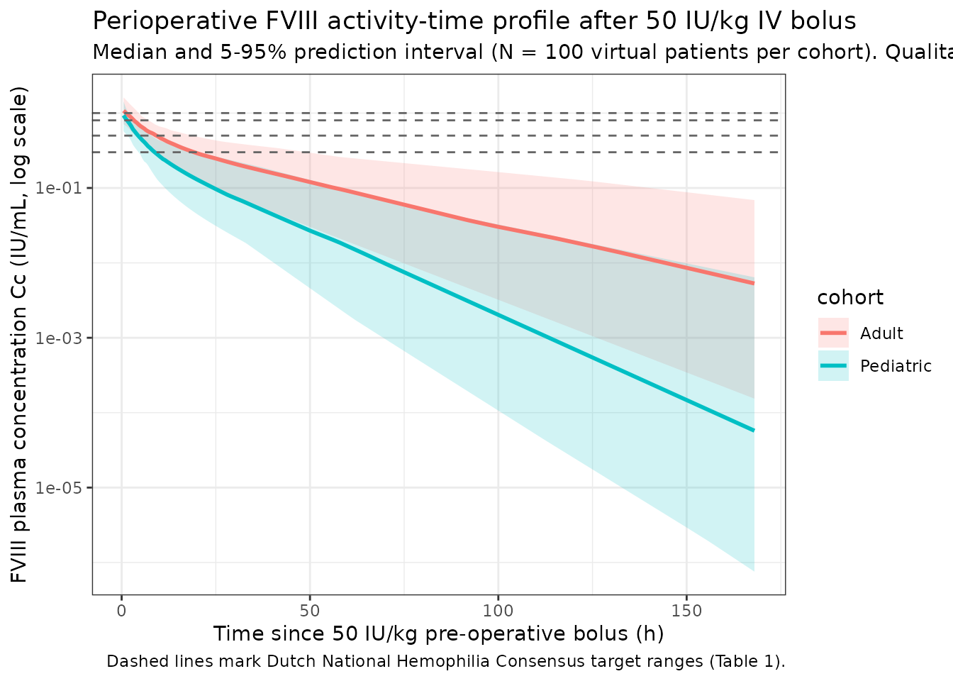
Replicate published projection – clearance vs age (typical value)
Hazendonk 2016 Figure 5A shows the typical-value FVIII clearance versus age in a body-weight-normalized form. The panel below reproduces the same projection: the packaged model’s typical CL evaluated across the perioperative cohort’s age range, holding body weight, blood group, and surgery severity at the paper’s reference values (68 kg, non-O, minor surgery). The four labeled ages 5, 20, 40, 55 y come from the paper’s narrative in Results (“Pharmacokinetic modeling”) and constitute a strict round-trip check.
age_grid <- seq(0.5, 78, by = 0.5)
cl_typical <- 150 * (age_grid / 40) ^ -0.17

anchor <- tibble::tibble(
  AGE = c(5, 20, 40, 55),
  CL  = c(214, 169, 150, 142)
)

ggplot(mapping = aes(age_grid, cl_typical)) +
  geom_line(linewidth = 1) +
  geom_point(data = anchor, aes(x = AGE, y = CL),
             colour = "firebrick", size = 3) +
  labs(
    x        = "Age (years)",
    y        = "Typical CL (mL/h/68 kg)",
    title    = "Typical FVIII clearance vs age (non-O, minor surgery, WT = 68 kg)",
    subtitle = "Line: packaged model. Red points: paper's narrative anchors at ages 5, 20, 40, 55 y (mL/h)."
  ) +
  theme_bw()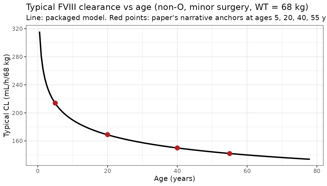
PKNCA validation
NCA parameters are computed per subject using PKNCA,
grouped by the age cohort so per-cohort summaries can be compared with
the paper’s derivation population. Half-life is anchored on the
elimination phase (log-linear regression on the terminal 3+ samples).
The paper states that the typical distribution and elimination
half-lives are approximately 4 and 25 hours (Hazendonk 2016 Discussion);
the PKNCA half.life interval below refers to the terminal
(elimination) phase.
sim_nca <- sim |>
  dplyr::filter(!is.na(Cc)) |>
  dplyr::select(id, cohort, time, Cc)

# Time-zero row per (id, cohort) -- FVIII activity is 0 at t = 0 for an
# IV bolus into the central compartment (endogenous baseline is fixed at
# zero for typical severe hemophilia; see Assumptions and deviations).
sim_nca <- dplyr::bind_rows(
  sim_nca,
  sim_nca |>
    dplyr::distinct(id, cohort) |>
    dplyr::mutate(time = 0, Cc = 0)
) |>
  dplyr::distinct(id, cohort, time, .keep_all = TRUE) |>
  dplyr::arrange(id, cohort, time)

conc_obj <- PKNCA::PKNCAconc(
  sim_nca, Cc ~ time | cohort + id,
  concu = "IU/mL",
  timeu = "h"
)

dose_df <- events |>
  dplyr::filter(evid == 1) |>
  dplyr::select(id, cohort, time, amt)

dose_obj <- PKNCA::PKNCAdose(
  dose_df, amt ~ time | cohort + id,
  doseu = "IU"
)

intervals <- data.frame(
  start      = 0,
  end        = Inf,
  cmax       = TRUE,
  tmax       = TRUE,
  aucinf.obs = TRUE,
  half.life  = TRUE
)

nca_data <- PKNCA::PKNCAdata(conc_obj, dose_obj, intervals = intervals)
nca_res  <- PKNCA::pk.nca(nca_data)

nca_summary <- as.data.frame(summary(nca_res))
knitr::kable(
  nca_summary,
  caption = "PKNCA summary per age cohort (single 50 IU/kg IV bolus)."
)| Interval Start | Interval End | cohort | N | Cmax (IU/mL) | Tmax (h) | Half-life (h) | AUCinf,obs (h*IU/mL) |
|---|---|---|---|---|---|---|---|
| 0 | Inf | Adult | 100 | 1.13 [28.6] | 0.000 [0.000, 0.000] | 28.8 [13.2] | 21.5 [48.0] |
| 0 | Inf | Pediatric | 100 | 0.986 [29.5] | 0.000 [0.000, 0.000] | 15.0 [5.24] | 9.76 [46.9] |
Comparison against published anchors
Hazendonk 2016 does not publish a formal NCA table but provides two
anchor quantities that the packaged model must reproduce: the
distribution and elimination half-lives calculated from the model’s
typical structural parameters (Hazendonk 2016 Discussion). These are
computed analytically from the two-compartment micro-constants
(alpha, beta) and then compared against the
paper’s narrative values below.
cl <- 0.150 # L/h at reference
vc <- 2.810 # L
q  <- 0.160 # L/h
vp <- 1.900 # L

k10 <- cl / vc
k12 <- q  / vc
k21 <- q  / vp

sum_k    <- k10 + k12 + k21
prod_k   <- k10 * k21
disc     <- sqrt(sum_k^2 - 4 * prod_k)
alpha    <- (sum_k + disc) / 2
beta     <- (sum_k - disc) / 2

t_half_distribution <- log(2) / alpha
t_half_elimination  <- log(2) / beta

tibble::tibble(
  Quantity = c("Distribution half-life (h)",
               "Elimination half-life (h)",
               "Typical CL at 68 kg, 40 y, non-O, minor surgery (mL/h)",
               "Typical V1 at 68 kg, 40 y (mL)",
               "Typical Q at 68 kg (mL/h)",
               "Typical V2 at 68 kg (mL)"),
  `This model (typical value)` = c(
    round(t_half_distribution, 2),
    round(t_half_elimination, 2),
    round(cl * 1000),
    round(vc * 1000),
    round(q * 1000),
    round(vp * 1000)
  ),
  `Hazendonk 2016 published anchor` = c(
    "~4 h (Discussion)",
    "~25 h (Discussion)",
    "150 (Table 4)",
    "2810 (Table 4)",
    "160 (Table 4)",
    "1900 (Table 4)"
  )
) |>
  knitr::kable(
    caption = "Analytical anchors: typical values from the packaged model vs Hazendonk 2016."
)| Quantity | This model (typical value) | Hazendonk 2016 published anchor |
|---|---|---|
| Distribution half-life (h) | 4.13 | ~4 h (Discussion) |
| Elimination half-life (h) | 25.86 | ~25 h (Discussion) |
| Typical CL at 68 kg, 40 y, non-O, minor surgery (mL/h) | 150.00 | 150 (Table 4) |
| Typical V1 at 68 kg, 40 y (mL) | 2810.00 | 2810 (Table 4) |
| Typical Q at 68 kg (mL/h) | 160.00 | 160 (Table 4) |
| Typical V2 at 68 kg (mL) | 1900.00 | 1900 (Table 4) |
Differences of a fraction of an hour on the half-lives reflect rounding to the Table 4 point estimates. The structural parameter values match by construction.
Assumptions and deviations
- Final model implemented; structural sub-models not implemented. Hazendonk 2016 Table 3 lists a nine-step model-building sequence culminating in the final covariate model (step 9). Only step 9 is packaged. Earlier variants (one-compartment; two-compartment without covariates; individual models with subsets of the retained covariates) are not implemented.
-
Center-specific residual error not implemented. The
paper stratifies residual error by treatment center: additive 0.15 IU/mL
+ proportional 0.18 for the majority centers 1, 2, 3 (Hazendonk 2016
Table 4) and 0.05 IU/mL + 0.23 for centers 4, 5. The packaged model uses
the centers-1-2-3 values (the majority group; three of five centers).
The center identities are not published, so users who want to reproduce
center-4/5 residual error should manually override
addSd = 0.05andpropSd = 0.23after loading the model withreadModelDb(). -
Individual endogenous baseline FVIII fixed at zero for
typical simulation. Hazendonk 2016 Structural model development
states “the structural model also accounted for the individual
endogenous baseline FVIII plasma concentration” and reports (Table 3)
that inclusion of that term reduced the OFV by ~17 units. The paper does
not report a typical population baseline value or the associated IIV;
per the inclusion criterion (severe or moderate hemophilia A, FVIII less
than 0.05 IU/mL), the typical severe-patient baseline is essentially
zero. The packaged model therefore has no baseline term in
Cc, and simulated activity at t = 0 for a severe / moderate patient is zero on IV bolus arms. Users who need a per-subject non-zero baseline (e.g. simulating moderate patients with 0.02-0.04 IU/mL endogenous FVIII) should add the offset in post-processing. - Inter-occasion variability not implemented. The paper tested IOV on CL and V1 but rejected it because of high shrinkage (34% and 46% respectively; Hazendonk 2016 Structural model development). The packaged model matches this choice and has no IOV term. For subjects undergoing multiple perioperative procedures, all occasions share the same individual etas.
- IIV on Q and V2 not identifiable in source; not implemented. The paper reports that IIV estimates on Q and V2 were “imprecise and accompanied by a large shrinkage of more than 40%”, so IIV was retained only on CL and V1. The packaged model reflects this: Q and V2 have no eta terms.
-
Fixed allometric exponents preserved. Hazendonk
2016 fixes the allometric exponents at the theory-based values 0.75
(clearances) and 1.0 (volumes) rather than estimating them. The packaged
model preserves these values with
fixed()wrappers so the fixed status is not lost. -
Covariate encoding. The paper’s Table 5 equation
writes categorical effects as
1.26 ^ blood_groupand0.93 ^ severity; for binary indicators these are algebraically equivalent to the linear forms(1 + 0.26 * BLOOD_GROUP_O)and(1 + (-0.07) * SURG_SEV_MAJOR), which the packaged model uses for parameter interpretability. The paper’s age effects are power-form(AGE/40)^-0.17and(AGE/40)^-0.09(Table 5); the packaged model uses the same power form. -
B-domain-deleted assay correction encoded as an
observation-level multiplier. The paper writes
C_pred,bdp = C_pred * (1 - theta_bdp)(Hazendonk 2016 Methods; theta_bdp = 0.34). The packaged model implements this asCc = (central / vc / 1000) * (1 - 0.34 * FORM_FVIII_BDD), so observations from BDD-product occasions (Refacto AF) show 66% of the underlying plasma concentration. Applies to any B-domain-deleted recombinant FVIII product; the paper’s cohort used only Refacto AF as the BDD product. -
Sex. Hemophilia A is X-linked recessive and the
cohort is essentially all-male; the paper does not tabulate sex
explicitly, so
sex_female_pctis set to 0 by inheritance. The packaged model carries no sex-related covariate. -
Concentration and dose units. The paper reports
FVIII activity in IU/mL and doses in IU throughout. The packaged model
uses dose in IU and V1 in L, so the observation equation includes an
internal
/ 1000factor to convert IU/L to IU/mL. Users supplying different dose / volume units must adjust accordingly. -
Continuous infusion regimens. The paper describes
both bolus and continuous infusion protocols but reports typical
population parameters independent of mode of infusion. Users simulating
continuous infusion should supply
rateorduron the event table’s dose row; the packaged model handles both.