Vancomycin (Fu 2021) • nlmixr2lib

Model and source

Citation: Fu X, Lin L, Huang L, Guo L. Clinical application of vancomycin population pharmacokinetics model in patients with hematological diseases and neutropenia. Biopharm Drug Dispos. 2021;42(9):427-434. doi:10.1002/bdd.2303
Description: Two-compartment IV population PK model for vancomycin in adolescent and adult Chinese patients with haematological diseases and neutropenia (Fu 2021). Clearance and intercompartmental clearance scale allometrically with body weight (exponent 0.75, reference 70 kg) and clearance additionally by a power of CKD-EPI creatinine clearance (reference 116 mL/min/1.73 m^2); both volumes scale linearly with body weight. Between-subject variability on CL and V1 only; the residual-error magnitude is not reported.
Article: https://doi.org/10.1002/bdd.2303 (open access, PMC9297986)

Fu 2021 reports a two-compartment population PK model of intravenous vancomycin in patients with haematological diseases and neutropenia, uses Monte Carlo simulation of it to pick a starting regimen by renal function (Figure 3), and then tests that starting regimen prospectively (Table 5). The model itself was first published in Chinese by Lin et al. (Chinese Journal of Clinical Pharmacology and Therapeutics, 2021); every value used here is printed in Fu 2021.

Population

The model was fit to 77 patients (42 male, 35 female) aged 17-83 years (mean 43.28) at Hainan General Hospital, Haikou, China, between January 2018 and January 2020 (Fu 2021 Results 3.1 and Table 1). All had a haematological disease – acute myeloid leukaemia (34), acute lymphoblastic leukaemia (16), lymphoma (10), aplastic anaemia (5), myelodysplastic syndrome (5), chronic myeloid leukaemia (4), multiple myeloma (2), chronic monocytic leukaemia (1) – and neutropenia (ANC < 0.5 x 10^9/L) during intermittent intravenous vancomycin; patients on any blood purification were excluded. Body weight was 56.84 +/- 11.09 kg (33.00-83.50) and CKD-EPI creatinine clearance 118.78 +/- 22.69 mL/min/1.73 m^2 (45.60-163.80): a lean cohort with high renal function. 80.74% of regimens were 1 g q12h; infusions ran at about 900 mg/h (Table 2). 109 troughs and 43 peaks were measured.

The same information is available programmatically:

str(rxode2::rxode(readModelDb("Fu_2021_vancomycin"))$population)
#> ℹ parameter labels from comments will be replaced by 'label()'
#> List of 15
#>  $ species         : chr "human"
#>  $ n_subjects      : int 77
#>  $ n_studies       : int 1
#>  $ age_range       : chr "17-83 years"
#>  $ age_median      : chr "43.28 years (mean, SD 15.88)"
#>  $ weight_range    : chr "33.00-83.50 kg"
#>  $ weight_median   : chr "56.84 kg (mean, SD 11.09)"
#>  $ sex_female_pct  : num 45.5
#>  $ race_ethnicity  : chr "Chinese (single-centre study in Haikou, Hainan, China; race not otherwise reported)"
#>  $ disease_state   : chr "Patients aged >= 14 years with haematological diseases and neutropenia (ANC < 0.5 x 10^9/L) receiving intermitt"| __truncated__
#>  $ dose_range      : chr "Intermittent IV vancomycin; 80.74% of regimens 1 g q12h, 7.34% 1 g q8h, 8.26% 0.5 g q6h, 1.83% 0.5 g q8h and 1."| __truncated__
#>  $ regions         : chr "China (Department of Hematology, Hainan General Hospital, Haikou; 1 January 2018 - 1 January 2020)"
#>  $ renal_function  : chr "CKD-EPI creatinine clearance 118.78 +/- 22.69 mL/min/1.73 m^2 (range 45.60-163.80); serum creatinine 53.66 +/- "| __truncated__
#>  $ n_concentrations: int 152
#>  $ notes           : chr "42 male and 35 female patients; 109 trough and 43 peak serum vancomycin concentrations (Siemens Viva-E immunoas"| __truncated__

Source trace

Equation / parameter	Value	Source location
Structure: two compartments, IV infusion into `central`	n/a	Fu 2021 Results 3.2.1
`CL = 6.84 * (WT/70)^0.75 * (CRCL/116)^0.895 * exp(eta1)`	n/a	Fu 2021 equation (6)
`V1 = 20.5 * (WT/70) * exp(eta2)`	n/a	Fu 2021 equation (7)
`Q = 15.2 * (WT/70)^0.75 * exp(eta3)`	n/a	Fu 2021 equation (8)
`V2 = 50 * (WT/70) * exp(eta4)`	n/a	Fu 2021 equation (9)
`lcl`	log(6.84 L/h)	Table 3 (RSE 4.5%)
`lvc`	log(20.5 L)	Table 3 (RSE 17.3%)
`lq`	log(15.2 L/h)	Table 3 (RSE 23.4%)
`lvp`	log(50 L)	Table 3 (RSE 27.2%)
`e_crcl_cl`	0.895	Table 3, theta CLCR_CL (RSE 14.3%)
`e_wt_cl`, `e_wt_q`	0.75, held constant	Equations (6) and (8); no estimate in Table 3
`e_wt_vc`, `e_wt_vp`	1, held constant	Equations (7) and (9); no estimate in Table 3
`etalcl`	0.178^2 = 0.031684	Table 3, eta1 = 17.8% (RSE 15%)
`etalvc`	0.33^2 = 0.1089	Table 3, eta2 = 33% (RSE 35.8%)
`etalq`, `etalvp`	0, held constant	Equations (8)-(9) carry eta3/eta4; no magnitude reported
`propSd`, `addSd`	0, held constant	Combined error (Methods 2.2, Results 3.2.1); no magnitude reported

Replicate Figure 3: first trough by renal function and regimen

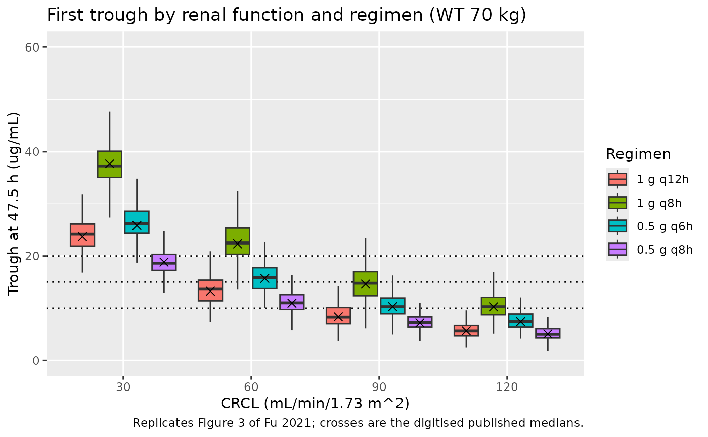
Fu 2021 Figure 3 shows the simulated vancomycin trough for four regimens (1 g q12h, 1 g q8h, 0.5 g q6h, 0.5 g q8h) at CKD-EPI creatinine clearance of 30, 60, 90 and 120 mL/min/1.73 m^2. Results 3.3 places the trough at “the 48th hour (the first C0)”, which the clinical arm samples 30 min before the next dose; the infusions are simulated at 1000 mg/h, the median rate in Table 2. The paper does not state the body weight of the simulated patients. The maintainers digitised the box medians from the figure, calibrating the y axis on its three dotted reference lines at 10, 15 and 20 ug/mL.

fig3_digitised <- tibble::tribble(
  ~CRCL, ~regimen,     ~paper_median,
  30,    "1 g q12h",   23.66,
  30,    "1 g q8h",    37.66,
  30,    "0.5 g q6h",  25.83,
  30,    "0.5 g q8h",  18.82,
  60,    "1 g q12h",   13.25,
  60,    "1 g q8h",    22.31,
  60,    "0.5 g q6h",  15.70,
  60,    "0.5 g q8h",  10.95,
  90,    "1 g q12h",    8.34,
  90,    "1 g q8h",    14.60,
  90,    "0.5 g q6h",  10.29,
  90,    "0.5 g q8h",   7.17,
  120,   "1 g q12h",    5.63,
  120,   "1 g q8h",    10.26,
  120,   "0.5 g q6h",   7.39,
  120,   "0.5 g q8h",   5.03
)

regimens <- tibble::tribble(
  ~regimen,    ~dose, ~tau,
  "1 g q12h",  1000,  12,
  "1 g q8h",   1000,   8,
  "0.5 g q6h",  500,   6,
  "0.5 g q8h",  500,   8
)
stopifnot(setequal(regimens$regimen, fig3_digitised$regimen))

# Build an event table: 1000 mg/h infusions every `tau` h from time 0 up to,
# but not including, 48 h, and observations on the `central` state.
make_events <- function(subjects, obs_times) {
  doses <- subjects |>
    dplyr::rowwise() |>
    dplyr::reframe(
      id = id,
      time = seq(0, 48 - 1e-6, by = tau),
      amt = dose,
      rate = 1000,
      evid = 1L
    )
  obs <- tidyr::crossing(id = subjects$id, time = obs_times) |>
    dplyr::mutate(amt = NA_real_, rate = NA_real_, evid = 0L)
  dplyr::bind_rows(doses, obs) |>
    dplyr::mutate(cmt = "central") |>
    dplyr::left_join(subjects, by = "id") |>
    dplyr::arrange(id, time, dplyr::desc(evid))
}

Typical-value prediction

mod <- readModelDb("Fu_2021_vancomycin")
mod_typical <- rxode2::zeroRe(mod)
#> ℹ parameter labels from comments will be replaced by 'label()'

grid_typical <- tidyr::crossing(regimens, CRCL = c(30, 60, 90, 120), WT = c(70, 57)) |>
  dplyr::mutate(id = dplyr::row_number())
ev_typical <- make_events(grid_typical |> dplyr::select(id, dose, tau, CRCL, WT), obs_times = 47.5)
stopifnot(!anyDuplicated(ev_typical[ev_typical$evid == 1L, c("id", "time")]))

sim_typical <- rxode2::rxSolve(mod_typical, events = ev_typical) |>
  as.data.frame() |>
  dplyr::filter(time == 47.5) |>
  dplyr::select(id, Cc) |>
  dplyr::left_join(grid_typical, by = "id")
#> ℹ omega/sigma items treated as zero: 'etalcl', 'etalvc', 'etalq', 'etalvp'
#> Warning: multi-subject simulation without without 'omega'

fig3_typical <- sim_typical |>
  dplyr::select(regimen, CRCL, WT, Cc) |>
  tidyr::pivot_wider(names_from = WT, values_from = Cc, names_prefix = "WT_") |>
  dplyr::inner_join(fig3_digitised, by = c("regimen", "CRCL")) |>
  dplyr::mutate(
    pct_70 = 100 * (WT_70 / paper_median - 1),
    pct_57 = 100 * (WT_57 / paper_median - 1)
  ) |>
  dplyr::arrange(CRCL, match(regimen, regimens$regimen))
stopifnot(nrow(fig3_typical) == 16L)

fig3_typical |>
  dplyr::mutate(dplyr::across(c(WT_70, WT_57, pct_70, pct_57), \(x) round(x, 1))) |>
  dplyr::select(CRCL, regimen, paper_median, WT_70, pct_70, WT_57, pct_57) |>
  dplyr::rename(
    "CRCL (mL/min/1.73 m^2)" = CRCL,
    "Regimen" = regimen,
    "Figure 3 median (ug/mL)" = paper_median,
    "Model, 70 kg (ug/mL)" = WT_70,
    "Diff, 70 kg (%)" = pct_70,
    "Model, 57 kg (ug/mL)" = WT_57,
    "Diff, 57 kg (%)" = pct_57
  ) |>
  knitr::kable(caption = "Typical-value 47.5-h trough against the digitised Figure 3 box medians.")

Typical-value 47.5-h trough against the digitised Figure 3 box medians.
CRCL (mL/min/1.73 m^2)	Regimen	Figure 3 median (ug/mL)	Model, 70 kg (ug/mL)	Diff, 70 kg (%)	Model, 57 kg (ug/mL)	Diff, 57 kg (%)
30	1 g q12h	23.66	24.1	2.0	28.6	21.0
30	1 g q8h	37.66	38.3	1.7	45.6	21.1
30	0.5 g q6h	25.83	26.1	1.2	31.1	20.5
30	0.5 g q8h	18.82	19.0	1.1	22.6	20.3
60	1 g q12h	13.25	13.5	1.8	15.7	18.7
60	1 g q8h	22.31	22.4	0.6	26.3	17.9
60	0.5 g q6h	15.70	15.6	-0.8	18.3	16.4
60	0.5 g q8h	10.95	11.1	1.2	13.0	18.6
90	1 g q12h	8.34	8.6	2.5	9.8	18.1
90	1 g q8h	14.60	14.8	1.5	17.2	17.8
90	0.5 g q6h	10.29	10.4	1.5	12.2	18.1
90	0.5 g q8h	7.17	7.3	1.6	8.5	17.9
120	1 g q12h	5.63	5.9	4.2	6.7	19.0
120	1 g q8h	10.26	10.5	2.8	12.2	18.7
120	0.5 g q6h	7.39	7.5	2.0	8.7	18.1
120	0.5 g q8h	5.03	5.2	2.7	6.0	18.5

At the 70 kg reference weight the typical-value trough lands on every one of the 16 Figure 3 medians to within about 5%, which is the resolution of the digitisation. At the cohort’s mean weight of 57 kg the predictions are uniformly about 16-21% higher, so the figure was simulated at the 70 kg reference. The check is deterministic, so it is gated tightly: a mis-transcribed clearance, renal exponent or volume, or a wrong trough time, moves whole rows of this table by tens of percent.

stopifnot(
  max(abs(fig3_typical$pct_70)) < 8,
  abs(median(fig3_typical$pct_70)) < 4,
  # The cohort-mean weight does not reproduce the figure, so the reading of
  # the unstated simulation weight is itself checked.
  median(fig3_typical$pct_57) > 10
)

Monte Carlo replicate

rxode2::rxSetSeed(2021)
n_per_cell <- 200L
grid_mc <- tidyr::crossing(regimens, CRCL = c(30, 60, 90, 120)) |>
  dplyr::mutate(cell = dplyr::row_number())
subjects_mc <- grid_mc |>
  tidyr::uncount(n_per_cell) |>
  dplyr::mutate(id = dplyr::row_number(), WT = 70)
ev_mc <- make_events(subjects_mc |> dplyr::select(id, dose, tau, CRCL, WT), obs_times = 47.5) |>
  dplyr::left_join(subjects_mc |> dplyr::select(id, regimen), by = "id")

sim_mc <- rxode2::rxSolve(mod, events = ev_mc, keep = c("regimen", "CRCL")) |>
  as.data.frame() |>
  dplyr::filter(time == 47.5)
#> ℹ parameter labels from comments will be replaced by 'label()'
#> ℹ omega/sigma items treated as zero: 'etalq', 'etalvp'

fig3_mc <- sim_mc |>
  dplyr::group_by(regimen, CRCL) |>
  dplyr::summarise(
    q25 = quantile(Cc, 0.25),
    sim_median = median(Cc),
    q75 = quantile(Cc, 0.75),
    .groups = "drop"
  ) |>
  dplyr::inner_join(fig3_digitised, by = c("regimen", "CRCL")) |>
  dplyr::mutate(pct = 100 * (sim_median / paper_median - 1))
stopifnot(nrow(fig3_mc) == 16L)

# Centre and envelope only, never the extremes of a simulated cohort.
stopifnot(
  abs(median(fig3_mc$pct)) < 6,
  quantile(abs(fig3_mc$pct), 0.9) < 12
)

sim_mc |>
  dplyr::mutate(regimen = factor(regimen, levels = regimens$regimen)) |>
  ggplot(aes(factor(CRCL), Cc, fill = regimen)) +
  geom_hline(yintercept = c(10, 15, 20), linetype = "dotted") +
  geom_boxplot(outlier.shape = NA, position = position_dodge(width = 0.85)) +
  geom_point(
    data = fig3_digitised |> dplyr::mutate(regimen = factor(regimen, levels = regimens$regimen)),
    aes(factor(CRCL), paper_median, group = regimen),
    position = position_dodge(width = 0.85), shape = 4, size = 2.5, inherit.aes = FALSE
  ) +
  coord_cartesian(ylim = c(0, 60)) +
  labs(
    x = "CRCL (mL/min/1.73 m^2)", y = "Trough at 47.5 h (ug/mL)", fill = "Regimen",
    title = "First trough by renal function and regimen (WT 70 kg)",
    caption = "Replicates Figure 3 of Fu 2021; crosses are the digitised published medians."
  )

Clinical application arm (Table 5)

Table 5 reports the first trough at 48 h in 74 further patients with CRCL >= 90 mL/min/1.73 m^2: 32 started on 1 g q8h (the model-guided group) and 42 on 1 g q12h (the empiric group). Each arm is simulated with 200 virtual patients whose weight and CRCL are drawn from normal distributions with the Table 5 means and SDs, truncated to the Table 5 ranges.

rtnorm <- function(n, mean, sd, lo, hi) {
  x <- rnorm(n, mean, sd)
  while (any(out <- x < lo | x > hi)) x[out] <- rnorm(sum(out), mean, sd)
  x
}
set.seed(2021)
n_arm <- 200L
arms <- dplyr::bind_rows(
  tibble::tibble(
    arm = "Model group, 1 g q8h", dose = 1000, tau = 8,
    WT = rtnorm(n_arm, 56.57, 9.40, 38.0, 72.0),
    CRCL = rtnorm(n_arm, 125.46, 17.57, 92.2, 164.8)
  ),
  tibble::tibble(
    arm = "Non-model group, 1 g q12h", dose = 1000, tau = 12,
    WT = rtnorm(n_arm, 56.43, 9.56, 48.0, 73.5),
    CRCL = rtnorm(n_arm, 119.63, 18.62, 93.6, 167.3)
  )
) |>
  dplyr::mutate(id = dplyr::row_number())
ev_t5 <- make_events(arms |> dplyr::select(id, dose, tau, CRCL, WT), obs_times = 47.5) |>
  dplyr::left_join(arms |> dplyr::select(id, arm), by = "id")
stopifnot(!anyDuplicated(unique(ev_t5[, c("id", "time", "evid")])))

rxode2::rxSetSeed(2021)
sim_t5 <- rxode2::rxSolve(mod, events = ev_t5, keep = "arm") |>
  as.data.frame() |>
  dplyr::filter(time == 47.5)
#> ℹ omega/sigma items treated as zero: 'etalq', 'etalvp'

t5 <- sim_t5 |>
  dplyr::group_by(arm) |>
  dplyr::summarise(sim_mean = mean(Cc), sim_sd = sd(Cc), sim_median = median(Cc), .groups = "drop") |>
  dplyr::left_join(
    tibble::tribble(
      ~arm,                         ~obs_mean, ~obs_sd,
      "Model group, 1 g q8h",       14.30,     4.73,
      "Non-model group, 1 g q12h",   8.02,     2.61
    ),
    by = "arm"
  ) |>
  dplyr::mutate(pct = 100 * (sim_mean / obs_mean - 1))
stopifnot(nrow(t5) == 2L)

t5 |>
  dplyr::mutate(dplyr::across(where(is.numeric), \(x) round(x, 2))) |>
  dplyr::select(arm, obs_mean, obs_sd, sim_mean, sim_sd, sim_median, pct) |>
  dplyr::rename(
    "Arm" = arm,
    "Observed mean (ug/mL)" = obs_mean,
    "Observed SD" = obs_sd,
    "Simulated mean (ug/mL)" = sim_mean,
    "Simulated SD" = sim_sd,
    "Simulated median" = sim_median,
    "Mean diff (%)" = pct
  ) |>
  knitr::kable(caption = "First trough at 48 h, Fu 2021 Table 5 versus simulation.")

First trough at 48 h, Fu 2021 Table 5 versus simulation.
Arm	Observed mean (ug/mL)	Observed SD	Simulated mean (ug/mL)	Simulated SD	Simulated median	Mean diff (%)
Model group, 1 g q8h	14.30	4.73	12.88	3.86	12.55	-9.95
Non-model group, 1 g q12h	8.02	2.61	6.82	2.28	6.37	-14.98


ratio_obs <- 14.30 / 8.02
ratio_sim <- t5$sim_mean[t5$arm == "Model group, 1 g q8h"] /
  t5$sim_mean[t5$arm == "Non-model group, 1 g q12h"]
c(observed = ratio_obs, simulated = ratio_sim)
#>  observed simulated 
#>  1.783042  1.888483

The model under-predicts both observed mean troughs, by roughly 10-15%. The direction is the same in both arms and the q8h/q12h ratio (observed 1.78) is reproduced closely, which points to a level difference between this prospective cohort and the model population rather than to a structural error. The observed SDs are larger than the simulated ones because the model carries no residual error (none is reported) and no variability on Q and V2. The gate checks the ratio, which every arm-level structural error would move, and records the level difference as a known deviation.

# Each arm mean has a Monte Carlo SE of about 2% at n = 200, so the ratio
# carries about 3%; the bound sits more than 3 SE beyond the ~6% realised
# here, while a mis-transcribed volume or clearance moves it by far more.
stopifnot(
  abs(ratio_sim / ratio_obs - 1) < 0.20,
  # Known deviation (both arms ~10-15% low): bounded, not widened to zero.
  all(t5$pct > -35 & t5$pct < 10)
)

Worked case (Results 3.5)

A 50-year-old woman of 47 kg with a CKD-EPI CRCL of 128.6 mL/min/1.73 m^2 received 1 g q12h; her first trough at 48 h was 6.0 ug/mL. The paper’s (individualised) prediction for 1 g q8h was 11.8 ug/mL and the measured trough after the switch 10.2 ug/mL.

case <- tibble::tibble(id = 1:2, dose = 1000, tau = c(12, 8), WT = 47, CRCL = 128.6)
sim_case <- rxode2::rxSolve(mod_typical, events = make_events(case, 47.5)) |>
  as.data.frame() |>
  dplyr::filter(time == 47.5)
#> ℹ omega/sigma items treated as zero: 'etalcl', 'etalvc', 'etalq', 'etalvp'
#> Warning: multi-subject simulation without without 'omega'
tibble::tibble(
  Regimen = c("1 g q12h", "1 g q8h"),
  "Typical-value prediction (ug/mL)" = round(sim_case$Cc, 1),
  "Reported (ug/mL)" = c("6.0 measured", "11.8 predicted, 10.2 measured")
) |>
  knitr::kable(caption = "Typical-value trough at 47.5 h for the Results 3.5 patient.")

Typical-value trough at 47.5 h for the Results 3.5 patient.
Regimen	Typical-value prediction (ug/mL)	Reported (ug/mL)
1 g q12h	6.8	6.0 measured
1 g q8h	12.7	11.8 predicted, 10.2 measured

The typical-value predictions (no individual adaptation) lie 8-25% above the reported values, as expected for a single patient.

PKNCA validation

The paper reports no NCA. PKNCA is therefore run on a steady-state dosing interval of the model-population virtual cohort for the two main regimens, and the AUC over the interval is checked against its closed form, AUC_tau,ss = Dose / CL, subject by subject.

set.seed(20211)
n_nca <- 200L
nca_subjects <- tidyr::crossing(
  tibble::tibble(
    sid = seq_len(n_nca),
    WT = rtnorm(n_nca, 56.84, 11.09, 33.0, 83.5),
    CRCL = rtnorm(n_nca, 118.78, 22.69, 45.6, 163.8)
  ),
  regimens |> dplyr::filter(dose == 1000)
) |>
  dplyr::mutate(id = dplyr::row_number(), treatment = regimen)

t_end <- 240 # 10 days: many terminal half-lives even at the lowest CRCL
nca_ev <- dplyr::bind_rows(
  nca_subjects |>
    dplyr::rowwise() |>
    dplyr::reframe(id = id, time = seq(0, t_end - tau, by = tau), amt = dose, rate = 1000, evid = 1L),
  nca_subjects |>
    dplyr::rowwise() |>
    dplyr::reframe(id = id, time = seq(t_end - tau, t_end, by = 0.25), amt = NA_real_, rate = NA_real_, evid = 0L)
) |>
  dplyr::mutate(cmt = "central") |>
  dplyr::left_join(nca_subjects |> dplyr::select(id, WT, CRCL, treatment, tau, dose), by = "id") |>
  dplyr::arrange(id, time, dplyr::desc(evid))
stopifnot(!anyDuplicated(unique(nca_ev[, c("id", "time", "evid")])))

rxode2::rxSetSeed(20211)
sim_nca_raw <- rxode2::rxSolve(
  mod, events = nca_ev, keep = c("treatment", "tau", "dose"),
  rtol = 1e-10, atol = 1e-12
) |>
  as.data.frame()
#> ℹ omega/sigma items treated as zero: 'etalq', 'etalvp'
stopifnot(!anyNA(sim_nca_raw$Cc))

# Re-anchor the last dosing interval at time 0 so PKNCA sees a single dose.
sim_nca <- sim_nca_raw |>
  dplyr::filter(!is.na(Cc)) |>
  dplyr::mutate(time = time - (t_end - tau)) |>
  dplyr::select(id, time, Cc, treatment, tau, cl)

conc_obj <- PKNCA::PKNCAconc(sim_nca, Cc ~ time | treatment + id)
dose_df <- nca_subjects |>
  dplyr::transmute(id, treatment, time = 0, amt = dose, tau)
dose_obj <- PKNCA::PKNCAdose(dose_df, amt ~ time | treatment + id)
intervals <- tibble::tibble(
  treatment = c("1 g q12h", "1 g q8h"),
  start = 0,
  end = c(12, 8),
  cmax = TRUE,
  cmin = TRUE,
  auclast = TRUE
)
nca_res <- PKNCA::pk.nca(PKNCA::PKNCAdata(conc_obj, dose_obj, intervals = intervals))

auc_check <- as.data.frame(nca_res) |>
  dplyr::filter(PPTESTCD == "auclast") |>
  dplyr::left_join(sim_nca |> dplyr::distinct(id, cl), by = "id") |>
  dplyr::mutate(closed_form = 1000 / cl, pct = 100 * (PPORRES / closed_form - 1))
stopifnot(nrow(auc_check) == 2L * n_nca)
# Same drawn parameters on both sides: only trapezoid error separates them.
stopifnot(max(abs(auc_check$pct)) < 1)

reference_auc <- auc_check |>
  dplyr::group_by(treatment) |>
  dplyr::summarise(auclast = median(closed_form), .groups = "drop")

cmp <- nlmixr2lib::ncaComparisonTable(
  simulated = nca_res,
  reference = reference_auc,
  by = "treatment",
  params = "auclast",
  units = c(auclast = "ug*h/mL"),
  tolerance_pct = 20
)
knitr::kable(cmp, caption = "Steady-state AUC over one dosing interval: PKNCA versus Dose / CL (median).")

Steady-state AUC over one dosing interval: PKNCA versus Dose / CL (median).
NCA parameter	treatment	Reference	Simulated	% diff
AUClast (ug*h/mL)	1 g q12h	168	168	-0.1%
AUClast (ug*h/mL)	1 g q8h	171	171	-0.0%


as.data.frame(nca_res) |>
  dplyr::filter(PPTESTCD %in% c("cmax", "cmin")) |>
  dplyr::group_by(treatment, PPTESTCD) |>
  dplyr::summarise(median = median(PPORRES), p05 = quantile(PPORRES, 0.05), p95 = quantile(PPORRES, 0.95), .groups = "drop") |>
  dplyr::mutate(dplyr::across(where(is.numeric), \(x) round(x, 1))) |>
  dplyr::rename("Regimen" = treatment, "Parameter" = PPTESTCD, "Median (ug/mL)" = median, "5th pct" = p05, "95th pct" = p95) |>
  knitr::kable(caption = "Steady-state Cmax and Cmin in the model-population virtual cohort.")

Steady-state Cmax and Cmin in the model-population virtual cohort.
Regimen	Parameter	Median (ug/mL)	5th pct	95th pct
1 g q12h	cmax	43.1	30.6	63.0
1 g q12h	cmin	6.6	3.1	13.9
1 g q8h	cmax	49.7	32.7	68.3
1 g q8h	cmin	12.3	6.9	22.0

For context, the observed concentrations in the model population (Table 2) were troughs of 9.07 +/- 5.47 ug/mL and peaks, drawn 0.5-1 h after the end of infusion, of 32.03 +/- 10.45 ug/mL, pooled over all regimens and sampling days. They are not NCA values and are not gated.

Assumptions and deviations

Residual error. Fu 2021 compared additive, proportional and combined residual-error models and carried the combined form into the base model, but reports no magnitude for either component in any model. Both propSd and addSd are held at zero; simulations are typical- or individual-level predictions without measurement noise. Supply your own values for VPC-style use.
IIV on Q and V2. Equations (8)-(9) include eta3 and eta4, but Table 3 and the base-model report give magnitudes only for eta1 (CL) and eta2 (V1). etalq and etalvp are held at zero rather than invented.
IIV scale. Table 3 lists eta1 = 17.8% and eta2 = 33% without saying whether they are sqrt(omega^2) x 100 or a log-normal CV. They are read as sqrt(omega^2) x 100 (variance = 0.031684 and 0.1089), consistent with the base model’s direct omega^2 report; the alternative log(1 + CV^2) reading gives 0.0312 and 0.1033, a difference that no reported quantity resolves.
Allometric exponents. 0.75 (CL, Q) and 1 (V1, V2) appear in the printed equations with no estimate, RSE or interval and are encoded as fixed.
Figure 3 simulation settings. The paper does not state the weight, infusion duration or trough time of its Monte Carlo simulation. The maintainers used 70 kg (the reference weight), 1000 mg/h infusions (the Table 2 maximum and modal rate) and a trough 30 min before the 48-h dose (Results 3.3 and 3.4). This combination reproduces all 16 published medians to within about 5%; the cohort-mean weight of 57 kg does not.
Figure 3 digitisation. Box medians were read by the maintainers from the figure at 300 dpi, calibrated on the dotted 10/15/20 ug/mL reference lines (about 0.1 ug/mL resolution).
Table 5 cohorts. Weight and CRCL were sampled independently from truncated normal distributions with the Table 5 means, SDs and ranges; their correlation is not reported. The simulated mean troughs fall about 10-15% below the observed means in both arms (a known deviation, discussed above).
Units. Doses are in mg and volumes in L, so Cc is in mg/L, identical to the ug/mL used throughout the paper.
Errata. Europe PMC lists no correction linked to Fu 2021 (PMID 34651308), and a search for a correction citing its DOI returned nothing, as of 2026-10-03.