Vedolizumab (Okamoto 2021) • nlmixr2lib

library(nlmixr2lib)
library(PKNCA)
#> 
#> Attaching package: 'PKNCA'
#> The following object is masked from 'package:stats':
#> 
#>     filter
library(rxode2)
#> rxode2 5.1.8 using 2 threads (see ?getRxThreads)
#>   no cache: create with `rxCreateCache()`
library(dplyr)
#> 
#> Attaching package: 'dplyr'
#> The following objects are masked from 'package:stats':
#> 
#>     filter, lag
#> The following objects are masked from 'package:base':
#> 
#>     intersect, setdiff, setequal, union
library(tidyr)
library(ggplot2)

Model and source

#> ℹ parameter labels from comments will be replaced by 'label()'
#> Warning: some etas defaulted to non-mu referenced, possible parsing error: etaiov_cl_1, etaiov_cl_2, etaiov_cl_3, etaiov_cl_4, etaiov_cl_5, etaiov_cl_6, etaiov_cl_7, etaiov_cl_8, etaiov_cl_9, etaiov_cl_10
#> as a work-around try putting the mu-referenced expression on a simple line

Citation: Okamoto H, Dirks NL, Rosario M, Hori T, Hibi T. Population pharmacokinetics of vedolizumab in Asian and non-Asian patients with ulcerative colitis and Crohn’s disease. Intest Res. 2021;19(1):95-105. doi:10.5217/ir.2019.09167 (PMC7873400).
Description: Two-compartment population PK model for vedolizumab (humanised anti-alpha4-beta7 integrin IgG1 monoclonal antibody) with parallel linear and Michaelis-Menten elimination, a time-varying anti-vedolizumab-antibody titer effect and an Asian-race effect on linear clearance, in Asian and non-Asian adults with moderately-to-severely active ulcerative colitis or Crohn’s disease (Okamoto 2021).
Article: https://doi.org/10.5217/ir.2019.09167 (open access, PMC7873400).
Errata: none found (PubMed and journal landing page checked 2026-09-27).

Okamoto 2021 refits the vedolizumab population PK model of Rosario 2015 (Rosario_2015_vedolizumab in this package) to a pool that adds three Japanese studies to GEMINI 1 and 2, re-assays anti-vedolizumab antibodies (AVA) with an electrochemiluminescence assay, and adds race (Asian vs non-Asian) and IBD diagnosis as covariates on linear clearance. The fit used Bayesian MCMC in NONMEM 7.3 with informative priors on Vmax, Km, Vp and Q taken from the earlier analysis; all Table 2 values are posterior medians.

Population

1,933 patients contributed 16,598 evaluable serum concentrations from five studies (Okamoto 2021 Table 1 and Results “Pharmacokinetic Analysis Dataset”): phase 1 CPH-001 (Japanese UC, n = 9), phase 3 CCT-101 (Japanese UC, n = 152), CCT-001 (Japanese CD, n = 63), GEMINI 1 (UC, n = 743) and GEMINI 2 (CD, n = 966). Median age was 36 years (range 17-79), median baseline weight 67 kg (28-172), median baseline albumin 3.80 g/dL (1.40-5.30); 47.3% were female, 53.2% had Crohn’s disease, 76.9% were White and 20.5% (n = 396) Asian, of whom 224 were Japanese patients in the three Japanese studies. 159 patients (8.2%) had at least one positive AVA titer. Dosing was 300 mg IV at weeks 0, 2 and 6 followed by 300 mg every 4 or 8 weeks in the phase 3 studies and 150 or 300 mg IV on days 1, 15 and 43 in CPH-001 (Supplementary Table 1).

The same information is available programmatically via readModelDb("Okamoto_2021_vedolizumab")$population.

Source trace

Every ini() value carries an in-file comment pointing to its source in inst/modeldb/specificDrugs/Okamoto_2021_vedolizumab.R; the table collects them in one place.

Equation / parameter	Value	Source location (Okamoto 2021)
`lcl` (AVA-negative)	`log(0.165)`	Table 2: AVA- CLL = 0.165 L/day
`lcl_adapos` (AVA-positive, titer 250)	`log(0.246)`	Table 2: AVA+ CLL = 0.246 L/day
`lvc`	`log(3.16)`	Table 2: Vc = 3.16 L
`lvp`	`log(1.84)`	Table 2: Vp = 1.84 L
`lq`	`log(0.161)`	Table 2: Q = 0.161 L/day
`lvmax`	`log(0.238)`	Table 2: Vmax = 0.238 mg/day
`lkm`	`log(0.851)`	Table 2: Km = 0.851 ug/mL
`e_wt_cl`	`0.472`	Table 2: CLL ~ WT
`e_alb_cl`	`-1.19`	Table 2: CLL ~ albumin
`e_ada_titer_cl`	`0.0713`	Table 2: CLL ~ AVA+ (titer power exponent)
`e_race_asian_cl`	`1.10`	Table 2: CLL ~ race: Asian
`e_ibd_cd_cl`	`0.990`	Table 2: CLL ~ diagnosis: CD
`e_wt_vc`	`0.466`	Table 2: Vc ~ WT
`e_wt_vp`, `e_wt_vmax`, `e_wt_q`	`fixed(1)`, `fixed(0.75)`, `fixed(0.75)`	Table 2: ‘Fixed’ rows
IIV variances CLL, Vc, Vp	`0.308^2`, `0.202^2`, `0.702^2`	Table 2: 30.8, 20.2, 70.2 %CV
IIV covariances	correlation x sd_i x sd_j	Table 2: CORR CLL-Vc 0.581, CLL-Vp 0.0188, Vc-Vp 0.371
IOV on CLL	`0.203^2 = 0.041209`	Table 2: IOV CLL 20.3 %CV
`propSd`	`sqrt(0.0318)`	Table 2: sigma^2 prop = 0.0318 (%CV 17.8)
AVA-positive definition	titer >= 10	Results “Final PK Model”
AVA titer form	`CLL(AVA+) * (titer / 250)^0.0713`	Results “Final PK Model” (“log-transformed power model normalized to a titer of 250”); confirmed against Figure 2 below
Weight / albumin references	70 kg, 4 g/dL	Table 2 footnote
Structure	2-cmt, zero-order IV input, parallel linear + Michaelis-Menten elimination	Results “Final PK Model”; Figure 1

Deterministic checks against the paper

Linear-elimination half-life

The paper reports a linear-elimination half-life of 24.7 days for the AVA-negative reference patient and 18.1 days for an AVA-positive patient at titer 250 (Results and Abstract). That is the beta-phase half-life of the linear two-compartment sub-system (CLL, Vc, Q, Vp) with the Michaelis-Menten pathway set aside. The check below takes the typical CLL directly from a model solve at the reference covariates, so it tests the packaged model() code, not a re-typed copy of the parameters.

mod_typ <- rxode2::zeroRe(mod)
#> Warning: some etas defaulted to non-mu referenced, possible parsing error: etaiov_cl_1, etaiov_cl_2, etaiov_cl_3, etaiov_cl_4, etaiov_cl_5, etaiov_cl_6, etaiov_cl_7, etaiov_cl_8, etaiov_cl_9, etaiov_cl_10
#> as a work-around try putting the mu-referenced expression on a simple line

# One observation row per covariate setting; `cl`, `vc`, `vp`, `q` are
# returned alongside Cc at each row.
ref_cov <- data.frame(
  WT = 70, ALB = 40, ADA_TITER = 0, RACE_ASIAN = 0, IBD_CD = 0, OCC = 1
)
typ_params <- function(cov) {
  ev <- cov |>
    mutate(id = seq_len(n()), time = 0, evid = 0, amt = 0, cmt = "central")
  rxode2::rxSolve(mod_typ, events = ev, returnType = "data.frame") |>
    select(cl, vc, vp, q)
}
beta_half_life <- function(cl, vc, vp, q) {
  k10 <- cl / vc
  k12 <- q / vc
  k21 <- q / vp
  s <- k10 + k12 + k21
  log(2) / ((s - sqrt(s^2 - 4 * k10 * k21)) / 2)
}

hl_cov <- bind_rows(ref_cov, mutate(ref_cov, ADA_TITER = 250))
hl <- typ_params(hl_cov) |>
  mutate(
    AVA = c("negative (titer < 10)", "positive (titer 250)"),
    simulated = beta_half_life(cl, vc, vp, q),
    published = c(24.7, 18.1)
  )
#> ℹ omega/sigma items treated as zero: 'etalcl', 'etalvc', 'etalvp', 'etaiov_cl_1', 'etaiov_cl_2', 'etaiov_cl_3', 'etaiov_cl_4', 'etaiov_cl_5', 'etaiov_cl_6', 'etaiov_cl_7', 'etaiov_cl_8', 'etaiov_cl_9', 'etaiov_cl_10'
#> Warning: multi-subject simulation without without 'omega'
hl |>
  select(AVA, cl, simulated, published) |>
  dplyr::rename(
    "AVA status" = AVA,
    "Typical CLL (L/day)" = cl,
    "Linear t1/2, model (day)" = simulated,
    "Linear t1/2, paper (day)" = published
  ) |>
  knitr::kable(digits = 3)

AVA status	Typical CLL (L/day)	Linear t1/2, model (day)	Linear t1/2, paper (day)
negative (titer < 10)	0.165	24.662	24.7
positive (titer 250)	0.246	18.117	18.1


# Both sides are deterministic; the only difference is the paper's rounding
# to one decimal.
stopifnot(all(abs(hl$simulated - hl$published) < 0.05))

Figure 2: covariate effects on linear clearance

Figure 2 of Okamoto 2021 plots CLL relative to the reference patient (70 kg, albumin 4 g/dL, non-Asian, UC, AVA-negative) with the median effect printed above each bar. The model’s typical CLL at each perturbed covariate setting, divided by the reference CLL, reproduces every printed median. The AVA titer rows are the check that settles the functional form of the titer effect: successive five-fold titer steps multiply CLL by the constant factor 5^0.0713 = 1.12, which is a power in titer normalised to 250 (on the log scale, linear in log(titer / 250)).

fig2 <- tribble(
  ~covariate, ~level, ~published,
  "Weight (kg)", 46, 0.82,
  "Weight (kg)", 57, 0.91,
  "Weight (kg)", 82, 1.08,
  "Weight (kg)", 106, 1.22,
  "Albumin (g/dL)", 2.7, 1.60,
  "Albumin (g/dL)", 3.4, 1.21,
  "Albumin (g/dL)", 4.1, 0.97,
  "Albumin (g/dL)", 4.5, 0.87,
  "AVA (titer)", 10, 1.19,
  "AVA (titer)", 50, 1.33,
  "AVA (titer)", 250, 1.49,
  "AVA (titer)", 1250, 1.67,
  "AVA (titer)", 6250, 1.87,
  "Race", 1, 1.10,
  "Diagnosis", 1, 0.99
)

fig2_cov <- ref_cov[rep(1, nrow(fig2)), ]
fig2_cov$WT[fig2$covariate == "Weight (kg)"] <- fig2$level[fig2$covariate == "Weight (kg)"]
# Albumin is in g/L in the model (canonical ALB); Figure 2 is in g/dL.
fig2_cov$ALB[fig2$covariate == "Albumin (g/dL)"] <- 10 * fig2$level[fig2$covariate == "Albumin (g/dL)"]
fig2_cov$ADA_TITER[fig2$covariate == "AVA (titer)"] <- fig2$level[fig2$covariate == "AVA (titer)"]
fig2_cov$RACE_ASIAN[fig2$covariate == "Race"] <- 1
fig2_cov$IBD_CD[fig2$covariate == "Diagnosis"] <- 1

cl_ref <- typ_params(ref_cov)$cl
#> ℹ omega/sigma items treated as zero: 'etalcl', 'etalvc', 'etalvp', 'etaiov_cl_1', 'etaiov_cl_2', 'etaiov_cl_3', 'etaiov_cl_4', 'etaiov_cl_5', 'etaiov_cl_6', 'etaiov_cl_7', 'etaiov_cl_8', 'etaiov_cl_9', 'etaiov_cl_10'
fig2$simulated <- typ_params(fig2_cov)$cl / cl_ref
#> ℹ omega/sigma items treated as zero: 'etalcl', 'etalvc', 'etalvp', 'etaiov_cl_1', 'etaiov_cl_2', 'etaiov_cl_3', 'etaiov_cl_4', 'etaiov_cl_5', 'etaiov_cl_6', 'etaiov_cl_7', 'etaiov_cl_8', 'etaiov_cl_9', 'etaiov_cl_10'
#> Warning: multi-subject simulation without without 'omega'
fig2 <- fig2 |>
  mutate(
    level = ifelse(covariate == "Race", "Asian", level),
    level = ifelse(covariate == "Diagnosis", "CD", level)
  )

fig2 |>
  mutate(simulated = round(simulated, 3)) |>
  dplyr::rename(
    "Covariate" = covariate,
    "Value" = level,
    "Relative CLL, Figure 2" = published,
    "Relative CLL, model" = simulated
  ) |>
  knitr::kable()

Covariate	Value	Relative CLL, Figure 2	Relative CLL, model
Weight (kg)	46	0.82	0.820
Weight (kg)	57	0.91	0.908
Weight (kg)	82	1.08	1.078
Weight (kg)	106	1.22	1.216
Albumin (g/dL)	2.7	1.60	1.596
Albumin (g/dL)	3.4	1.21	1.213
Albumin (g/dL)	4.1	0.97	0.971
Albumin (g/dL)	4.5	0.87	0.869
AVA (titer)	10	1.19	1.185
AVA (titer)	50	1.33	1.329
AVA (titer)	250	1.49	1.491
AVA (titer)	1250	1.67	1.672
AVA (titer)	6250	1.87	1.876
Race	Asian	1.10	1.100
Diagnosis	CD	0.99	0.990


# Deterministic: Figure 2 prints two decimals, so a correct model differs
# only by rounding (< 0.005 plus a margin for the paper's own rounding of
# the Table 2 exponents).
stopifnot(all(abs(fig2$simulated - fig2$published) < 0.008))

fig2 |>
  mutate(label = paste(covariate, level)) |>
  mutate(label = factor(label, levels = rev(label))) |>
  ggplot(aes(y = label)) +
  annotate("rect", xmin = 0.75, xmax = 1.25, ymin = -Inf, ymax = Inf,
           fill = "grey85") +
  geom_vline(xintercept = 1) +
  geom_point(aes(x = simulated), size = 2.5, colour = "#1f77b4") +
  geom_point(aes(x = published), shape = 4, size = 2.5) +
  labs(
    x = "CLL relative to the reference patient",
    y = NULL,
    caption = paste(
      "Replicates the medians of Figure 2 of Okamoto 2021.",
      "Circles: packaged model; crosses: printed medians.",
      "Grey band: +/-25% region of clinical unimportance."
    )
  ) +
  theme_bw()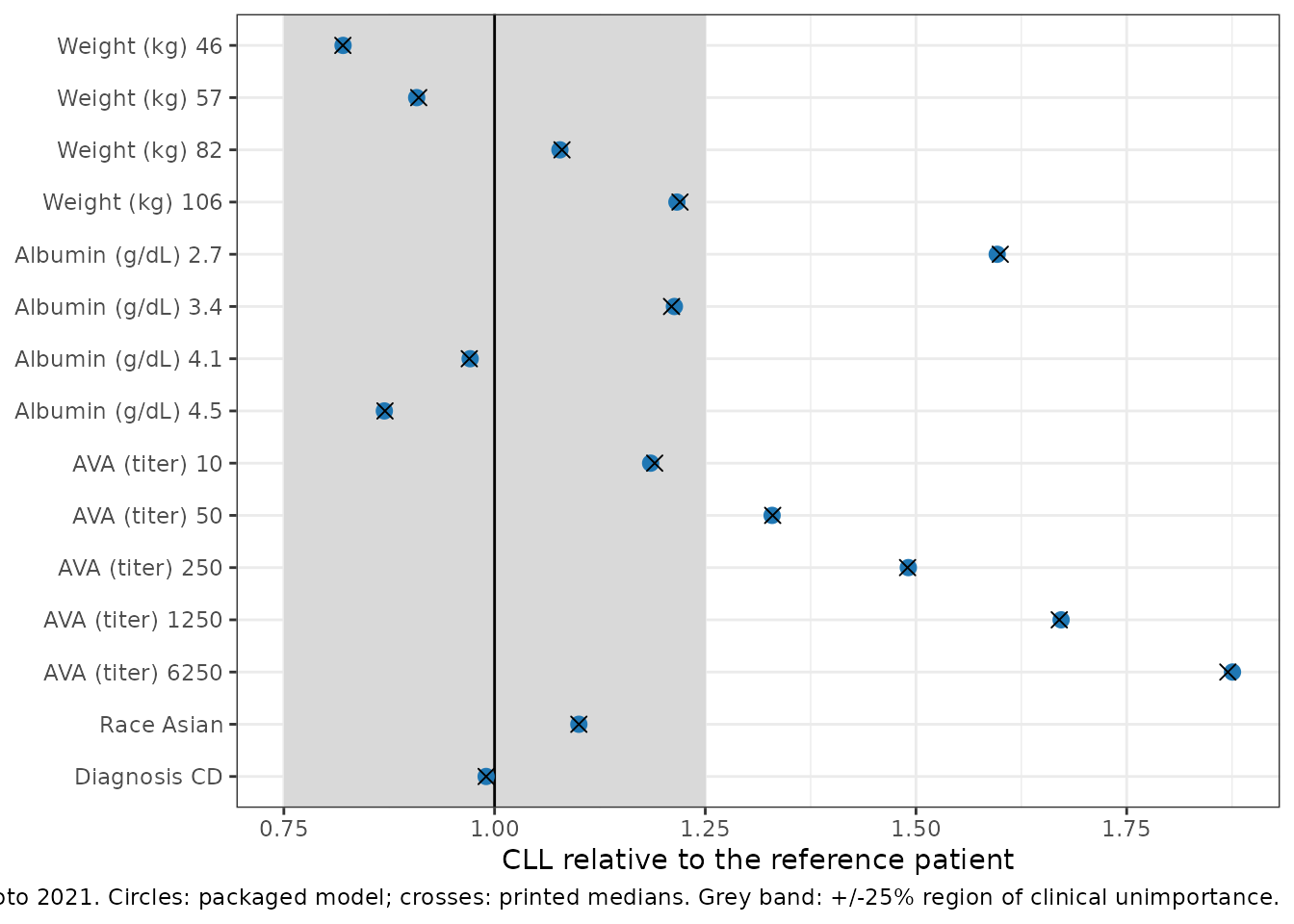

Virtual cohort

The observed data are not public. Two virtual cohorts of 200 patients each approximate the Asian and non-Asian subgroups. Weight and albumin are drawn log-normally around medians taken from Table 1 (Japanese studies: about 57 kg and 3.9 g/dL; GEMINI: about 69 kg and 3.75 g/dL), with draws outside the observed ranges (28-172 kg, 1.4-5.3 g/dL) rejected and redrawn rather than clamped. Each cohort is 53% Crohn’s disease. About 8% of patients are AVA-positive with a constant titer drawn from the titers Figure 2 evaluates; the rest carry ADA_TITER = 0. Weight, albumin and titer are held constant over time here, although the model accepts them as time-varying columns.

rxode2::rxSetSeed(20210195)
set.seed(20210195)

# Log-normal draws restricted to [lo, hi] by rejection (never clamped, so the
# distribution inside the range keeps its shape).
rlnorm_range <- function(n, median, sdlog, lo, hi) {
  out <- rlnorm(n, log(median), sdlog)
  bad <- out < lo | out > hi
  while (any(bad)) {
    out[bad] <- rlnorm(sum(bad), log(median), sdlog)
    bad <- out < lo | out > hi
  }
  out
}

make_cohort <- function(n, asian, wt_median, alb_median, id_offset) {
  ada_pos <- rbinom(n, 1, 0.082)
  data.frame(
    id = id_offset + seq_len(n),
    group = ifelse(asian == 1, "Asian", "Non-Asian"),
    WT = rlnorm_range(n, wt_median, 0.22, 28, 172),
    ALB = 10 * rlnorm_range(n, alb_median, 0.13, 1.4, 5.3),
    ADA_TITER = ifelse(ada_pos == 1, sample(c(10, 50, 250, 1250), n, TRUE), 0),
    RACE_ASIAN = asian,
    IBD_CD = rbinom(n, 1, 0.53)
  )
}

cohort <- bind_rows(
  make_cohort(200, asian = 1, wt_median = 57, alb_median = 3.9, id_offset = 0L),
  make_cohort(200, asian = 0, wt_median = 69, alb_median = 3.75, id_offset = 200L)
)
stopifnot(!anyDuplicated(cohort$id))

cohort |>
  group_by(group) |>
  summarise(
    n = n(),
    `median WT (kg)` = median(WT),
    `median ALB (g/dL)` = median(ALB) / 10,
    `AVA-positive (%)` = 100 * mean(ADA_TITER >= 10),
    `CD (%)` = 100 * mean(IBD_CD),
    .groups = "drop"
  ) |>
  knitr::kable(digits = 1)

group	n	median WT (kg)	median ALB (g/dL)	AVA-positive (%)	CD (%)
Asian	200	59.2	3.9	7.5	54.0
Non-Asian	200	68.4	3.7	5.5	48.5

Simulation

Label regimen: 300 mg IV over 30 minutes at weeks 0, 2 and 6, then every 8 weeks through week 46 (8 doses). Each dosing interval is one occasion (OCC 1-8), so the inter-occasion variability on CLL is re-drawn at every dose, matching the paper’s occasion definition (a dosing interval with at least one PK sample).

dose_days <- c(0, 2, 6, 14, 22, 30, 38, 46) * 7
tau <- 56
obs_days <- sort(unique(c(
  seq(0, 54 * 7, by = 7),
  dose_days + 30 / 1440, # end of infusion
  dose_days[8] + c(0.5, 1, 2, 4, 7, 14, 21, 28, 35, 42, 49, 56)
)))

occ_of <- function(t) findInterval(t, dose_days, left.open = FALSE)

doses <- cohort |>
  tidyr::crossing(time = dose_days) |>
  mutate(evid = 1, amt = 300, rate = 300 / (30 / 1440), cmt = "central")
obs <- cohort |>
  tidyr::crossing(time = obs_days) |>
  mutate(evid = 0, amt = 0, rate = 0, cmt = "central")
events <- bind_rows(doses, obs) |>
  mutate(OCC = pmax(1L, occ_of(time))) |>
  arrange(id, time, desc(evid))

sim <- rxode2::rxSolve(
  mod,
  events = events,
  keep = c("group"),
  returnType = "data.frame"
)

sim |>
  filter(time > 0) |>
  group_by(group, time) |>
  summarise(
    p05 = quantile(Cc, 0.05),
    p50 = median(Cc),
    p95 = quantile(Cc, 0.95),
    .groups = "drop"
  ) |>
  ggplot(aes(time / 7, p50, colour = group, fill = group)) +
  geom_ribbon(aes(ymin = p05, ymax = p95), alpha = 0.15, colour = NA) +
  geom_line() +
  scale_y_log10() +
  labs(
    x = "Time since first dose (weeks)",
    y = "Vedolizumab serum concentration (ug/mL)",
    colour = NULL, fill = NULL,
    caption = paste(
      "Median and 5th-95th percentiles, 200 virtual patients per group,",
      "300 mg IV at weeks 0, 2, 6 then every 8 weeks."
    )
  ) +
  theme_bw()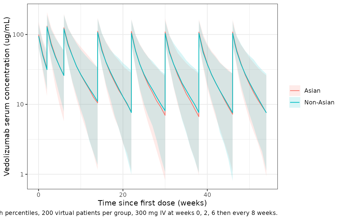

PKNCA validation

Steady-state NCA over the last maintenance interval (week 46 to week 54), by race group. Okamoto 2021 does not print NCA or exposure summaries, so there is no published column to compare against; the table documents the exposure the model implies and shows the small race difference the paper describes as not clinically important. Ctrough is the concentration at the end of the interval (week 54). It is not the interval minimum: the week-46 pre-dose sample belongs to the previous occasion, whose independent IOV draw makes the two troughs differ, so the minimum of the pair would be biased low. For the reference patient (70 kg, albumin 4 g/dL, AVA-negative, UC) the typical-value trough on this regimen is about 9.6 ug/mL, essentially the same as the predecessor Rosario_2015_vedolizumab model.

nca_conc <- sim |>
  filter(!is.na(Cc), time >= dose_days[8]) |>
  mutate(time = time - dose_days[8], treatment = group) |>
  select(id, time, Cc, treatment)

nca_dose <- doses |>
  filter(time == dose_days[8]) |>
  transmute(id, time = 0, amt, treatment = group)

conc_obj <- PKNCA::PKNCAconc(nca_conc, Cc ~ time | treatment + id)
dose_obj <- PKNCA::PKNCAdose(nca_dose, amt ~ time | treatment + id)
intervals <- data.frame(
  start = 0, end = tau,
  cmax = TRUE, ctrough = TRUE, auclast = TRUE
)
nca <- PKNCA::pk.nca(PKNCA::PKNCAdata(conc_obj, dose_obj, intervals = intervals))

nca_summary <- as.data.frame(nca$result) |>
  group_by(treatment, PPTESTCD) |>
  summarise(median = median(PPORRES), .groups = "drop") |>
  tidyr::pivot_wider(names_from = PPTESTCD, values_from = median)

nca_summary |>
  dplyr::rename(
    "Group" = treatment,
    "Cmax,ss (ug/mL)" = cmax,
    "Ctrough,ss (ug/mL)" = ctrough,
    "AUCtau,ss (ug*day/mL)" = auclast
  ) |>
  knitr::kable(digits = 1)

Group	AUCtau,ss (ug*day/mL)	Cmax,ss (ug/mL)	Ctrough,ss (ug/mL)
Asian	1641.4	108.7	7.6
Non-Asian	1631.5	104.1	7.6

ref_trough <- function(model_name, cov) {
  ev <- bind_rows(
    data.frame(time = dose_days, evid = 1, amt = 300,
               rate = 300 / (30 / 1440), cmt = "central"),
    data.frame(time = 54 * 7, evid = 0, amt = 0, rate = 0, cmt = "central")
  ) |>
    bind_cols(cov)
  m <- rxode2::zeroRe(rxode2::rxode(readModelDb(model_name)))
  sim_ref <- rxode2::rxSolve(m, events = ev, returnType = "data.frame")
  sim_ref$Cc[sim_ref$time == 54 * 7]
}
trough_okamoto <- ref_trough("Okamoto_2021_vedolizumab", ref_cov)
#> ℹ parameter labels from comments will be replaced by 'label()'
#> Warning: some etas defaulted to non-mu referenced, possible parsing error: etaiov_cl_1, etaiov_cl_2, etaiov_cl_3, etaiov_cl_4, etaiov_cl_5, etaiov_cl_6, etaiov_cl_7, etaiov_cl_8, etaiov_cl_9, etaiov_cl_10
#> as a work-around try putting the mu-referenced expression on a simple line
#> Warning: some etas defaulted to non-mu referenced, possible parsing error: etaiov_cl_1, etaiov_cl_2, etaiov_cl_3, etaiov_cl_4, etaiov_cl_5, etaiov_cl_6, etaiov_cl_7, etaiov_cl_8, etaiov_cl_9, etaiov_cl_10
#> as a work-around try putting the mu-referenced expression on a simple line
#> ℹ omega/sigma items treated as zero: 'etalcl', 'etalvc', 'etalvp', 'etaiov_cl_1', 'etaiov_cl_2', 'etaiov_cl_3', 'etaiov_cl_4', 'etaiov_cl_5', 'etaiov_cl_6', 'etaiov_cl_7', 'etaiov_cl_8', 'etaiov_cl_9', 'etaiov_cl_10'
trough_rosario <- ref_trough(
  "Rosario_2015_vedolizumab",
  data.frame(
    WT = 70, ALB = 40, AGE = 40, SCORE_CALPRO = 700, SCORE_CDAI = 300,
    SCORE_PMAYO = 6, IBD_CD = 0, PRIOR_TNF = 0, ADA_POS = 0, CONMED_AZA = 0,
    CONMED_MP = 0, CONMED_MTX = 0, CONMED_AMINO = 0
  )
)
#> ℹ parameter labels from comments will be replaced by 'label()'
#> ℹ omega/sigma items treated as zero: 'etalcl', 'etalvc', 'etalvmax'
data.frame(
  Model = c("Okamoto 2021", "Rosario 2015"),
  `Typical week-54 trough (ug/mL)` = c(trough_okamoto, trough_rosario),
  check.names = FALSE
) |>
  knitr::kable(digits = 2)

Model	Typical week-54 trough (ug/mL)
Okamoto 2021	9.60
Rosario 2015	9.69


# Deterministic typical-value solves.
stopifnot(
  abs(trough_okamoto - 9.6) < 0.1,
  abs(trough_okamoto / trough_rosario - 1) < 0.05
)

A structural check on the PKNCA result: at steady state and with the Michaelis-Menten pathway minor at these concentrations (Km = 0.851 ug/mL against troughs near 10 ug/mL), AUCtau is close to Dose / CL. The saturable pathway can only remove extra drug, so the median ratio of AUCtau to Dose / CL must sit below 1, and only modestly below it.

cl_ss <- sim |>
  filter(time == dose_days[8] + 1) |>
  select(id, cl)
auc_chk <- as.data.frame(nca$result) |>
  filter(PPTESTCD == "auclast") |>
  inner_join(cl_ss, by = "id") |>
  mutate(ratio = PPORRES / (300 / cl))

auc_chk |>
  group_by(treatment) |>
  summarise(`median AUCtau / (Dose / CL)` = median(ratio), .groups = "drop") |>
  knitr::kable(digits = 3)

treatment	median AUCtau / (Dose / CL)
Asian	0.965
Non-Asian	0.954


# Centre-of-distribution gate (medians, not cohort extremes): a wrong
# clearance, dose or unit moves the median by tens of
# percent; the MM pathway alone keeps it modestly below 1.
stopifnot(
  median(auc_chk$ratio) < 1,
  median(auc_chk$ratio) > 0.8
)

Assumptions and deviations

IIV scale. Table 2 reports IIV and IOV as %CV. The residual row shows the paper’s convention (sigma^2 = 0.0318 is printed as %CV = 17.8, i.e. 100 * sqrt(variance)), which is also the convention of the predecessor Rosario 2015 analysis by the same group, so the variances are (%CV / 100)^2. Covariances are built from the printed correlations. The Abstract quotes 19% for the Vc IIV; Table 2 (20.2%) is used.
Number of occasions. The paper defines an occasion as a dosing interval with at least one PK sample but does not state how many there are. Ten occasion etas (etaiov_cl_1 to etaiov_cl_10) sharing one variance are encoded; ten covers the densest per-patient PK schedule in the pooled studies (GEMINI every-4-weeks arm, Supplementary Table 1). Records with OCC outside 1-10 receive no IOV.
AVA titer form. The text calls the AVA effect “a log-transformed power model normalized to a titer of 250”. The packaged form, CLL(AVA+) * (titer / 250)^0.0713 for titer >= 10 and the separate AVA-negative CLL otherwise, reproduces all five AVA medians of Figure 2 (above), which rules out a power in log(titer). Negative records are coded ADA_TITER = 0.
Albumin units. The paper uses g/dL with reference 4 g/dL; the model takes the package’s canonical ALB in g/L with the equivalent reference 40 g/L.
Infusion duration. The paper does not state it; the simulations use the labelled 30-minute infusion. It has no effect on the model parameters.
Screened but not modelled. Age and sex were in the dataset but not in the full covariate model; they are listed under covariatesDataExcluded.
Figure 3 (distributions of individual post-hoc CLL by race and diagnosis) needs the observed data and is not reproduced.

Reference

Okamoto H, Dirks NL, Rosario M, Hori T, Hibi T. Population pharmacokinetics of vedolizumab in Asian and non-Asian patients with ulcerative colitis and Crohn’s disease. Intest Res. 2021;19(1):95-105. doi:10.5217/ir.2019.09167 (PMC7873400).