Scopolamine (Liem-Moolenaar 2011)
Source:vignettes/articles/LiemMoolenaar_2011_scopolamine.Rmd
LiemMoolenaar_2011_scopolamine.RmdModel and source
Liem-Moolenaar et al. (2011) characterised the pharmacokinetics and pharmacodynamics of scopolamine after a single 0.5 mg intravenous infusion in 85 healthy male volunteers (pooled from two four-way crossover studies). A two-compartment population PK model (Table 2) described scopolamine disposition, and ten independent effect-compartment linear-concentration PK/PD models (Table 3) characterised central-nervous-system effects across neurophysiological, subjective, and motor endpoints. The PD endpoints spanned three orders of magnitude in equilibration half-life, from heart rate (16.8 min) to finger tapping (649 min), supporting the paper’s conclusion that multiple distinct functional pathways of the cholinergic system are engaged.
- Citation: Liem-Moolenaar M, de Boer P, Timmers M, Schoemaker RC, van Hasselt JGC, Schmidt S, van Gerven JMA. Pharmacokinetic-pharmacodynamic relationships of central nervous system effects of scopolamine in healthy subjects. Br J Clin Pharmacol. 2011;71(6):886-898.
- Article: https://doi.org/10.1111/j.1365-2125.2011.03936.x
Population
Two double-blind, placebo-controlled, four-way crossover studies enrolled 90 healthy male volunteers aged 18-55 years with BMI 18-28.5 kg/m^2 at the Centre for Human Drug Research (Leiden, the Netherlands); 85 subjects completed the study and were evaluable for PK/PD. Scopolamine 0.5 mg was given as a 15-minute IV infusion at time zero; pharmacodynamic measurements were performed twice pre-dose and at approximately 0.75, 1.0, 1.5, 2.0, 2.5, 3.5, 4.5, 6.5, and 8.5 h post dose. Plasma scopolamine concentrations were drawn at 0.5, 0.75, 1.0, 2.5, and 6.5 h post dose by LC-MS/MS (LLOQ = 10 pg/mL). The same individuals supplied both the PK fit and the ten endpoint-specific PK/PD fits (sequential modelling: empirical-Bayes individual PK parameters were carried into the PK/PD analyses).
The same metadata is available programmatically via
readModelDb("LiemMoolenaar_2011_scopolamine")$population.
Source trace
Per-parameter origin is recorded as an in-file comment next to each
ini() entry in
inst/modeldb/specificDrugs/LiemMoolenaar_2011_scopolamine.R.
The table below collects them in one place.
| Equation / parameter | Value | Source location |
|---|---|---|
lcl (CL) |
2.53 L/min | Table 2 |
lvc (Vc) |
66.3 L | Table 2 |
lq (Q) |
4.78 L/min | Table 2 |
lvp (Vp = Vss - Vc) |
183.7 L | Table 2 (Vss = 250 L; Vp derived) |
etalcl (CV 15.4%) |
0.023568 | Table 2 IIVar |
etalvc (CV 36.6%) |
0.125855 | Table 2 IIVar |
etalq (CV 8.9%) |
0.007885 | Table 2 IIVar |
propSd (PK residual) |
0.102 | Table 2 (SD/mean) |
| Effect-compartment ODE | dCe/dt = ke0 (Cc - Ce) | Methods (Results: PK-PD relationships) |
| Linear PD relationship | E = intercept + slope * Ce | Methods (Results: PK-PD relationships) |
| HR intercept | 55.2 beats/min | Table 3 |
| HR slope | -0.00675 | Table 3 (footnote on slope-sign parameterisation) |
| HR t1/2,keo | 16.8 min | Table 3 |
| HR residual error | 0.103 | Table 3 |
| SPV intercept | 485 deg/s | Table 3 |
| SPV slope | -0.0737 | Table 3 |
| SPV t1/2,keo | 65.1 min | Table 3 |
| Adaptive tracking intercept | 0.0479 % | Table 3 |
| Adaptive tracking slope | -0.0217 | Table 3 |
| Adaptive tracking t1/2,keo | 86.6 min | Table 3 |
| VAS external intercept | 0.34 log mm | Table 3 |
| VAS external slope | 0.000633 | Table 3 |
| VAS external t1/2,keo | 161 min | Table 3 |
| Body sway intercept | 2.4 log mm | Table 3 |
| Body sway slope | 0.00147 | Table 3 |
| Body sway t1/2,keo | 181 min | Table 3 |
| VAS alertness intercept | 53.6 mm | Table 3 |
| VAS alertness slope | -0.0622 | Table 3 |
| VAS alertness t1/2,keo | 199 min | Table 3 |
| VAS internal intercept | 0.336 log mm | Table 3 |
| VAS internal slope | 0.000331 | Table 3 |
| VAS internal t1/2,keo | 200 min | Table 3 |
| Smooth pursuit intercept | 3.1 % | Table 3 |
| Smooth pursuit slope | -0.0264 | Table 3 |
| Smooth pursuit t1/2,keo | 221 min | Table 3 |
| VAS feeling high intercept | 0.328 log mm | Table 3 |
| VAS feeling high slope | 0.00313 | Table 3 |
| VAS feeling high t1/2,keo | 483 min | Table 3 |
| Finger tapping intercept | 63.4 taps/10s | Table 3 |
| Finger tapping slope | -0.0797 | Table 3 |
| Finger tapping t1/2,keo | 649 min | Table 3 |
| Finger tapping time slope | 19.3 /day | Table 3 footnote ** |
Virtual cohort and event-table builder
A single healthy male subject receives a 0.5 mg scopolamine IV infusion over 15 minutes (matching the source dosing regimen). Time is in minutes; the observation window covers 0-510 min (0-8.5 h) to match the published PD sampling schedule.
The model has eleven outputs (Cc for plasma scopolamine
plus ten PD endpoints). For multi-output simulation, each output
requires its own observation rows tagged with the corresponding
cmt value; we build the event table by combining one dose
row with eleven sets of observation rows.
endpoints <- c("Cc", "hr", "spv", "tracking", "vasext", "bodysway",
               "vasalert", "vasint", "smoothpursuit", "vashigh", "tapping")
obs_times <- seq(0, 510, by = 5)

build_events <- function(n = 1L) {
  dose_rows <- data.frame(
    id   = seq_len(n),
    time = 0,
    amt  = 0.5,
    cmt  = "central",
    dur  = 15,
    evid = 1L
  )
  obs_rows <- expand.grid(
    id   = seq_len(n),
    time = obs_times,
    cmt  = endpoints,
    stringsAsFactors = FALSE
  )
  obs_rows$amt  <- 0
  obs_rows$dur  <- NA_real_
  obs_rows$evid <- 0L
  rbind(
    dose_rows[, c("id", "time", "amt", "cmt", "dur", "evid")],
    obs_rows[,  c("id", "time", "amt", "cmt", "dur", "evid")]
  )
}

events <- build_events(n = 1L)
Simulation
mod <- readModelDb("LiemMoolenaar_2011_scopolamine")

# Typical-value replication: zero out random effects so the simulation
# reproduces the published Table 2 / Table 3 typical-value curves.
mod_typical <- rxode2::zeroRe(mod)
#> ℹ parameter labels from comments will be replaced by 'label()'

# rxSolve returns one row per (id, time, cmt) observation tag and carries
# every model-derived variable as a column. Filter to a single CMT so we
# have one row per time point with all eleven outputs available as columns.
sim <- rxode2::rxSolve(mod_typical, events = events, returnType = "data.frame")
#> ℹ omega/sigma items treated as zero: 'etalcl', 'etalvc', 'etalq', 'etalintercept_hr', 'etaslope_hr', 'etalke0_hr', 'etalintercept_spv', 'etaslope_spv', 'etalintercept_tracking', 'etaslope_tracking', 'etalke0_tracking', 'etalintercept_vasext', 'etaslope_vasext', 'etalke0_vasext', 'etalintercept_bodysway', 'etaslope_bodysway', 'etalke0_bodysway', 'etalintercept_vasalert', 'etaslope_vasalert', 'etalke0_vasalert', 'etalintercept_vasint', 'etaslope_vasint', 'etalke0_vasint', 'etalintercept_smoothpursuit', 'etaslope_smoothpursuit', 'etalke0_smoothpursuit', 'etalintercept_vashigh', 'etaslope_vashigh', 'etalke0_vashigh', 'etalintercept_tapping', 'etaslope_tapping', 'etalke0_tapping'
sim_wide <- sim |>
  dplyr::filter(CMT == min(CMT)) |>
  dplyr::select(time, dplyr::all_of(endpoints))

sim_long <- sim_wide |>
  tidyr::pivot_longer(
    cols      = dplyr::all_of(endpoints),
    names_to  = "endpoint",
    values_to = "value"
  )
Replicate published PK profile (Figure 2)
The paper reports Cmax = 1287 pg/mL at ~30 min and a terminal half-life of ~1.5 h after the 0.5 mg IV infusion.
sim_pk <- sim_wide |>
  dplyr::select(time, Cc)

ggplot(sim_pk, aes(time, Cc)) +
  geom_line(linewidth = 0.6) +
  labs(x = "Time (min)", y = "Scopolamine concentration (pg/mL)",
       title = "Scopolamine PK after 0.5 mg IV infusion over 15 min")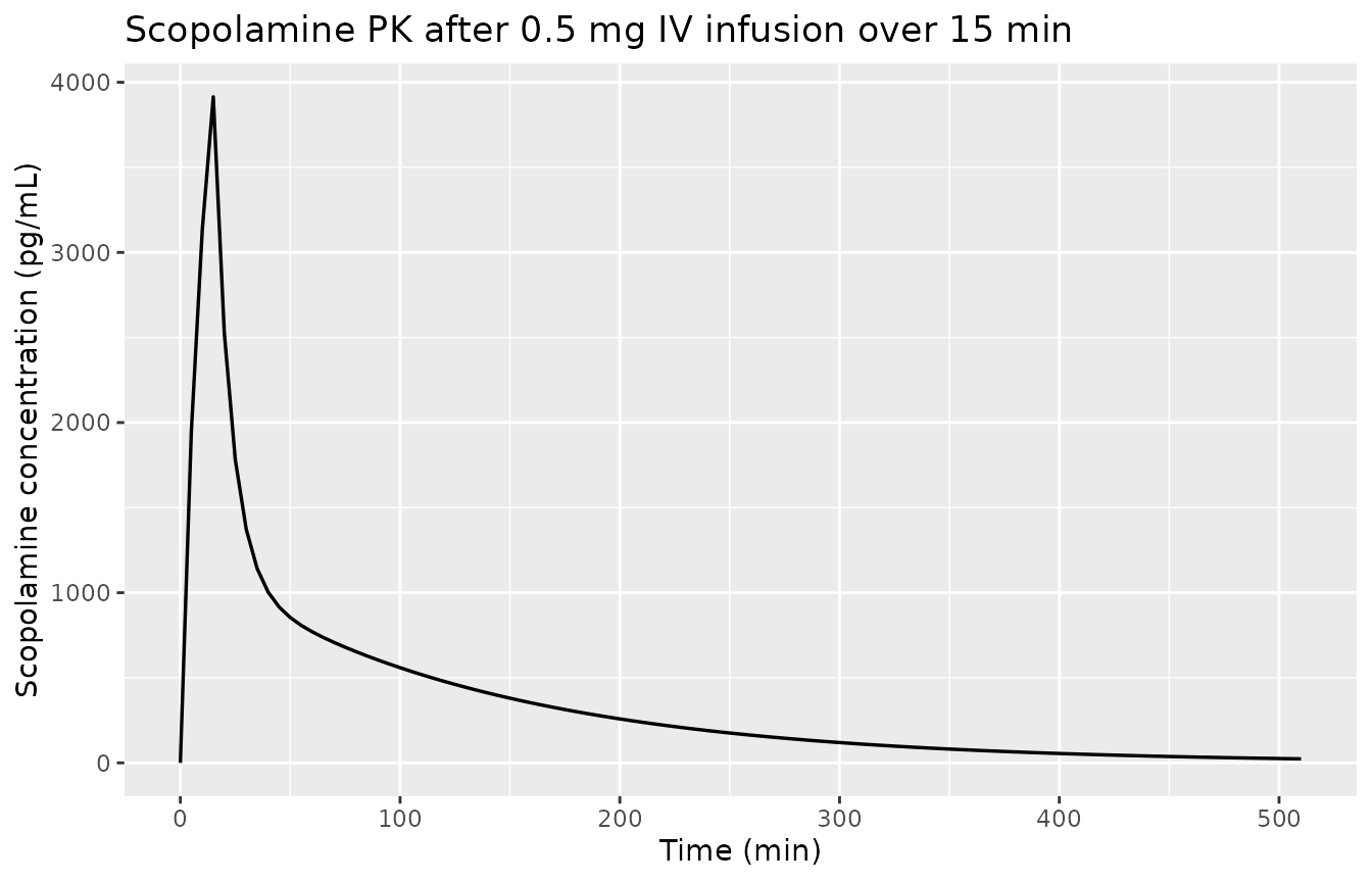
Scopolamine plasma concentration vs. time. Replicates Liem-Moolenaar 2011 Figure 2 (two-compartment model trace).
PKNCA validation of plasma scopolamine
The paper sampled scopolamine plasma concentrations at 30, 45, 60, 150, and 390 min after the start of the IV infusion (0.5, 0.75, 1.0, 2.5, and 6.5 h). Note that the first sampling occurred 15 min AFTER the end of the 15-min infusion, so the reported “Cmax” of 1287 pg/mL is the 30-min observation rather than the true peak of the underlying model (which a denser simulation grid shows occurs at the end of infusion, t = 15 min, with Cc ~ 3.9 ng/mL). To make a faithful comparison we restrict the NCA input to the paper’s sampling grid.
paper_sample_times <- c(30, 45, 60, 150, 390)

sim_nca <- sim_pk |>
  dplyr::filter(time %in% paper_sample_times) |>
  dplyr::mutate(id = 1L, treatment = "0.5 mg IV") |>
  dplyr::select(id, time, Cc, treatment)

# Anchor the AUC integration window with a pre-dose Cc = 0 row at t = 0.
sim_nca <- dplyr::bind_rows(
  data.frame(id = 1L, time = 0, Cc = 0, treatment = "0.5 mg IV"),
  sim_nca
) |>
  dplyr::distinct(id, treatment, time, .keep_all = TRUE) |>
  dplyr::arrange(id, treatment, time)

conc_obj <- PKNCA::PKNCAconc(sim_nca, Cc ~ time | treatment + id)

dose_df <- data.frame(id = 1L, time = 0, amt = 0.5, treatment = "0.5 mg IV")
dose_obj <- PKNCA::PKNCAdose(dose_df, amt ~ time | treatment + id)

intervals <- data.frame(
  start      = 0,
  end        = Inf,
  cmax       = TRUE,
  tmax       = TRUE,
  aucinf.obs = TRUE,
  half.life  = TRUE
)

nca_data <- PKNCA::PKNCAdata(conc_obj, dose_obj, intervals = intervals)
nca_res  <- PKNCA::pk.nca(nca_data)
Comparison against published NCA
The paper reports Cmax = 1287 pg/mL (mean across 85 subjects, observed at 30 min), AUC0-inf = 2752 pg/mL.h (mean), and terminal half-life 1.5 h (range 1.2-2.49 h). PKNCA returns AUC in units of (pg/mL) * min; we convert to pg/mL.h for direct comparison.
nca_results <- as.data.frame(nca_res$result)
pull_param <- function(p) {
  v <- nca_results$PPORRES[nca_results$PPTESTCD == p]
  if (length(v) == 0) NA_real_ else v[1]
}
sim_cmax_nca <- pull_param("cmax")
sim_tmax_nca <- pull_param("tmax")
sim_auc_min  <- pull_param("aucinf.obs")
sim_auc_hr   <- sim_auc_min / 60
sim_thalf    <- pull_param("half.life") / 60

cmp <- tibble::tribble(
  ~`NCA parameter`,      ~Simulated,            ~Published,
  "Cmax (pg/mL)",        sprintf("%.0f", sim_cmax_nca), "1287",
  "Tmax (min)",          sprintf("%.0f", sim_tmax_nca), "~30",
  "AUC0-inf (pg/mL.h)",  sprintf("%.0f", sim_auc_hr),   "2752",
  "t1/2 (h)",            sprintf("%.2f", sim_thalf),    "1.5 (range 1.2-2.49)"
)

knitr::kable(
  cmp,
  caption = "Simulated typical-value vs. published NCA for 0.5 mg IV scopolamine (Liem-Moolenaar 2011 Table 2 + Results, Pharmacokinetics).",
  align   = c("l", "r", "r")
)| NCA parameter | Simulated | Published |
|---|---|---|
| Cmax (pg/mL) | 1373 | 1287 |
| Tmax (min) | 30 | ~30 |
| AUC0-inf (pg/mL.h) | 2484 | 2752 |
| t1/2 (h) | 1.49 | 1.5 (range 1.2-2.49) |
Replicate published PD time courses (Figure 1)
For each PD endpoint, the typical-value time course shows the effect- compartment-mediated delay relative to the plasma PK profile. Figure 1 of Liem-Moolenaar 2011 plots all endpoints; we faceted-plot the endpoint-level simulation.
endpoint_labels <- c(
  hr            = "Heart rate (beats/min)",
  spv           = "Saccadic peak velocity (deg/s)",
  tracking      = "Adaptive tracking (%)",
  vasext        = "VAS external (log mm)",
  bodysway      = "Body sway (log mm)",
  vasalert      = "VAS alertness (mm)",
  vasint        = "VAS internal (log mm)",
  smoothpursuit = "Smooth pursuit (%)",
  vashigh       = "VAS feeling high (log mm)",
  tapping       = "Finger tapping (taps/10s)"
)
ep_order <- names(endpoint_labels)

sim_pd <- sim_long |>
  dplyr::filter(endpoint != "Cc") |>
  dplyr::mutate(endpoint = factor(endpoint, levels = ep_order,
                                  labels = endpoint_labels[ep_order]))

ggplot(sim_pd, aes(time, value)) +
  geom_line(linewidth = 0.5) +
  facet_wrap(~endpoint, scales = "free_y", ncol = 2) +
  labs(x = "Time (min)", y = "Predicted typical value")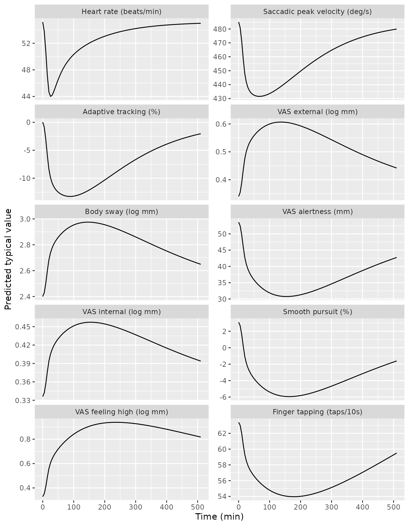
Typical-value PD time courses for the ten PK/PD endpoints. Replicates Liem-Moolenaar 2011 Figure 1 (predicted-line component).
Approximate peak PD shifts vs. published Table 1
The paper’s Table 1 reports mean placebo-vs-scopolamine differences averaged across the 0-8.5 h observation window (or 0-22 h for hormones). For the modelled endpoints, the magnitudes can be sanity-checked by the predicted excursion from the typical-value baseline at peak effect- compartment concentration. The comparison is approximate because the paper’s Table 1 mean is a time-average difference rather than a peak, and the model’s effect-compartment lag means peak Ce occurs after Cmax.
peak_shifts <- sim_pd |>
  dplyr::group_by(endpoint) |>
  dplyr::summarise(
    baseline = value[which.min(abs(time - 0))],
    max_val  = max(value, na.rm = TRUE),
    min_val  = min(value, na.rm = TRUE),
    extremum = ifelse(abs(max_val - baseline) >= abs(min_val - baseline),
                      max_val, min_val),
    delta    = extremum - baseline,
    .groups  = "drop"
  ) |>
  dplyr::select(-max_val, -min_val)

knitr::kable(
  peak_shifts |>
    dplyr::mutate(
      baseline = round(baseline, 3),
      extremum = round(extremum, 3),
      delta    = round(delta, 3)
    ),
  caption = "Simulated typical-value baseline and peak excursion per endpoint (0-510 min window). Compare in magnitude to the time-averaged scopolamine-vs-placebo differences in Liem-Moolenaar 2011 Table 1."
)| endpoint | baseline | extremum | delta |
|---|---|---|---|
| Heart rate (beats/min) | 55.200 | 44.017 | -11.183 |
| Saccadic peak velocity (deg/s) | 485.000 | 431.562 | -53.438 |
| Adaptive tracking (%) | 0.048 | -13.262 | -13.309 |
| VAS external (log mm) | 0.340 | 0.607 | 0.267 |
| Body sway (log mm) | 2.400 | 2.975 | 0.575 |
| VAS alertness (mm) | 53.600 | 30.744 | -22.856 |
| VAS internal (log mm) | 0.336 | 0.457 | 0.121 |
| Smooth pursuit (%) | 3.100 | -5.947 | -9.047 |
| VAS feeling high (log mm) | 0.328 | 0.939 | 0.611 |
| Finger tapping (taps/10s) | 63.400 | 53.967 | -9.433 |
Assumptions and deviations
- The paper reports Vss (steady-state volume of distribution = Vc + Vp) with 7.2% inter-individual variability rather than Vp directly. The packaged model derives Vp = Vss - Vc = 250 - 66.3 = 183.7 L and applies no eta to Vp; the Vc IIV (36.6%) carries the dominant volume-of- distribution variability. This is a faithful encoding of the published numerical values but loses the small additional Vss variability the paper reported.
- For the ten PD endpoints, the inter-individual variability on the
linear-PD slope is encoded as a multiplicative log-normal effect
(
slope_i = slope_pop * exp(etaslope)) so the sign of the population slope is preserved. This is the standard approach when CV% is reported for a parameter that can take either sign. - For saccadic peak velocity the paper reported zero IIV on the
effect-compartment equilibration half-life (Table 3 IICV 0.0%); no eta
is applied to
lke0_spv. - The heart-rate residual error is encoded as proportional (10.3%
fraction of mean) rather than additive (which would correspond to 0.103
beats/min, an implausibly tight SD); this is consistent with the paper’s
stated LTBS-style residual modelling for PK and with the similarity of
the reported HR residual to the PK residual SD/mean. Other linear-scale
PD endpoints (SPV, adaptive tracking, VAS alertness, smooth pursuit,
finger tapping) are encoded as additive on their reported units.
Log-scale endpoints (VAS external, body sway, VAS internal, VAS feeling
high) are encoded with additive residuals on the log-mm scale; the model
output for those endpoints is the log value (the user can
exp()for the linear mm value). - The paper used “log mm” units for body sway, VAS external, VAS internal, and VAS feeling high without explicitly stating the logarithm base; the published intercept for body sway (2.4 log mm) matches log10(268 mm) where 268 mm was the placebo-arm body sway in Table 1. The model encodes the raw values as reported and leaves base interpretation to the user.
- The finger-tapping additive time slope of 19.3 (taps per 10 s) per
day captures within-visit learning / practice effects and is applied as
time_slope * (t / 1440)with t in minutes. No IIV is applied to this time slope (the paper did not report one). - Adaptive tracking and smooth pursuit had separate placebo models per the paper (Methods: “a separate placebo model in the analysis for those parameters where a placebo response was observed”); those placebo models are not tabulated and are not part of the packaged model. The scopolamine PK/PD encoded here is the structural effect-compartment relationship reported in Table 3.
- The paper reports a four-way crossover design that included a placebo arm and active experimental glycinergic compounds; only the scopolamine treatment data informed the PK/PD models published in the article and only the scopolamine arm is encoded in this model.