Osimertinib target-site PBPK (van der Gaag 2025)
Source:vignettes/articles/vanderGaag_2025_osimertinib_pbpk.Rmd
vanderGaag_2025_osimertinib_pbpk.RmdModel and source
- Citation: van der Gaag S, Jordens T, Yaqub M, Grijseels R, van Valkengoed DW, de Langen EN, van den Broek R, Thijssen VLJL, de Langen AJ, Kouwenhoven MCM, Bahce I, Westerman BA, Hendrikse NH, Bartelink IH. Physiologically Based Pharmacokinetic Model of Tyrosine Kinase Inhibitors to Predict Target Site Penetration, with PET-Guided Verification. CPT Pharmacometrics Syst Pharmacol. 2025;14(5):918-928. doi:10.1002/psp4.70006. Organ volumes, intracellular-water volumes and blood flows from Appendix S2 Table S1; body/pH/haematocrit constants from Table S2; tissue fractional volumes from Table S3; lysosomal fractions, acidic phospholipid and EGFR concentrations from Table S4; liver and lung cell-type composition from Table S5; osimertinib physicochemical and clearance parameters from Appendix S3 Table S6; tumor and EGFR binding parameters from main-text Table 1; Kpu equations from Appendix S4 Suppl Eq 1-6; whole-body ODEs from Appendix S5 Suppl Eq 7-20; EGFR-binding and free-receptor-fraction equations from main-text Equations 1-2. The tumor extracellular-water pH term and the tumor 100% residual-cell composition are inherited from the explicitly cited predecessor model Bartelink IH, et al. Physiologically Based Pharmacokinetic (PBPK) Modeling to Predict PET Image Quality of Three Generations EGFR TKI in Advanced-Stage NSCLC Patients. Pharmaceuticals (Basel). 2022;15(7):796. doi:10.3390/ph15070796 (Supplement section VC and supplement note 9).
- Article: https://doi.org/10.1002/psp4.70006
- Supplement (Appendices S1-S10, all equations and parameter tables):
https://doi.org/10.1002/psp4.70006 Supporting
Information file
PSP4-14-918-s001.docx - Predecessor / framework model: Bartelink et al., Pharmaceuticals 2022;15(7):796, https://doi.org/10.3390/ph15070796
Osimertinib is a third-generation EGFR tyrosine kinase inhibitor and
the standard first-line therapy for advanced NSCLC with an activating
EGFR mutation. Whether enough drug reaches the tumour is not
answerable from plasma PK alone, and microdosed
[11C]C-osimertinib PET can measure tissue uptake directly –
but only at a microdose, where EGFR binding and metabolism are far from
saturated. This model exists to bridge that gap: a whole-body PBPK model
carrying explicit, saturable EGFR binding so that a 2.7 ug intravenous
microdose and an 80 mg oral therapeutic dose can be simulated with the
same parameter set.
Two features distinguish it from a conventional PBPK model.
- No fitted partition coefficients. Every tissue-to-plasma partition coefficient is computed inside the model from the Rodgers and Rowland moderate-to-strong-base equations (Suppl Eq 1-6), combining osimertinib’s pKa, logD, fraction unbound and blood-to-plasma ratio with each tissue’s fractional water, lipid, acidic-phospholipid and lysosomal composition. Nothing in this model was estimated from the clinical data.
- Saturable target binding as explicit states. Each of the ten EGFR-expressing tissues carries a second state holding drug covalently bound to EGFR, so receptor occupancy is a simulated output rather than an assumption.
Population
pop <- rxode2::rxode(readModelDb("vanderGaag_2025_osimertinib_pbpk"))$population
str(pop, max.level = 1)
#> List of 11
#>  $ species       : chr "human"
#>  $ n_subjects    : int 4
#>  $ n_studies     : int 2
#>  $ age_range     : chr NA
#>  $ weight_range  : chr "single 87.5 kg reference individual (Table S2); the model is deterministic and is not stratified by body size"
#>  $ sex_female_pct: num NA
#>  $ race_ethnicity: chr NA
#>  $ disease_state : chr "advanced-stage (stage 3-4) non-small cell lung cancer with an activating EGFR mutation (exon 19 deletion or exo"| __truncated__
#>  $ dose_range    : chr "2.7 ug (280 MBq) intravenous [11C]C-osimertinib microdose, and 80 mg oral osimertinib once daily"
#>  $ regions       : chr "Netherlands (Amsterdam UMC)"
#>  $ notes         : chr "This is a bottom-up whole-body PBPK model: every parameter is a literature or in-vitro value and none was estim"| __truncated__
The model is deterministic and represents a single 87.5 kg reference
individual (Table S2); it carries no between-subject variability.
Verification used two independent data sets. Four patients with
advanced-stage NSCLC and an activating EGFR mutation (exon 19
deletion or exon 21 L858R) who had progressed on a first-generation
EGFR-TKI each underwent two dynamic [11C]C-osimertinib PET
scans, one on and one off concomitant TKI; because concomitant TKI did
not change uptake the scans were pooled. Three of the four also had a
whole-body static PET at 60 min, giving brain, kidney, liver, lung,
spleen and tumour concentrations. Separately, plasma concentration-time
profiles from 10 healthy volunteers given a single 80 mg oral dose were
digitised from phase 1 study D5160C00001.
The authors adopted a 3-fold rather than the customary 2-fold prediction-error window, justified by the small sample size and the high inter- and intra-patient variability of tissue PK.
Source trace
Every ini() entry in
inst/modeldb/specificDrugs/vanderGaag_2025_osimertinib_pbpk.R
carries an in-file comment naming its source location. The table below
collects the model’s structural provenance in one place.
| Equation / parameter group | Source location |
|---|---|
| Organ total volumes, intracellular-water volumes, blood flows | Appendix S2, Table S1 |
| Body weight, pH of plasma / EW / IW / lysosomes / blood cells, haematocrit | Appendix S2, Table S2 |
Tissue fractional volumes fnl, fnp,
few, fiw
|
Appendix S2, Table S3 |
| Lysosomal fractional volumes, acidic phospholipids, tissue EGFR concentrations | Appendix S2, Table S4 |
Liver and lung cell-type composition (flys,
fcell, lysosomal pH) |
Appendix S2, Table S5 |
pKa, logD, logPV, Fu, blood-to-plasma ratio,
Ka, F, CL_int, CL_R,
Ka_bc
|
Appendix S3, Table S6 |
Tumour EGFR, tumour pH_EW, tumour blood flow, virtual tumour volume,
Kon / Koff (wild-type, mutated, 50/50) |
Main text, Table 1 |
Kpu for intracellular water, lipids, acidic
phospholipids, lysosomes; Kp = Kpu * Fu
|
Appendix S4, Suppl Eq 1-6 |
| Non-eliminating tissue, lung, venous and arterial ODEs | Appendix S5, Suppl Eq 7-10 |
| EGFR-expressing tissue ODEs (bound and unbound states) | Appendix S5, Suppl Eq 11-12 |
| Absorption; gut ODE | Appendix S5, Suppl Eq 13-14 |
Hepatic clearance and CL_int derivation; liver and
kidney ODEs |
Appendix S5, Suppl Eq 15-20 |
| EGFR association / dissociation; free-receptor fraction; tissue EGFR concentration | Main text, Equations 1, 2, 3 |
| Tumour extracellular-water pH term; tumour 100% residual-cell composition | Bartelink 2022 supplement, section VC and note 9 |
Two items come from the predecessor paper rather than from van der Gaag 2025. Both are flagged in Assumptions and deviations below; the current paper states explicitly that the NSCLC hallmarks “have been described and verified previously by Bartelink et al.”, and that paper is the cited framework source.
Derived partition coefficients
Because the Kp values are computed rather than
tabulated, the first validation step is to inspect them. The chunk below
solves the model once and reads the derived quantities straight out of
the model body.
mod <- readModelDb("vanderGaag_2025_osimertinib_pbpk")

MW      <- 500      # g/mol, Table S6
nmol_mg <- 1e6 / MW # mg -> nmol

# A minimal solve: one observation record on a real ODE state so that every
# algebraic observable is evaluated and returned.
probe <- data.frame(
  id = 1L, time = 0, amt = NA_real_, evid = 0L, cmt = "venous"
)
kp_probe <- rxode2::rxSolve(mod, probe, useLinCmt = FALSE) |> as.data.frame()

tissues <- c("adipose", "brain", "gut", "heart", "kidney", "liver",
             "lung", "tumor", "pancreas", "muscle", "skin", "spleen", "other")

# Read the composite tissue-to-blood coefficient kb = Kpu * Fu / BP, which the
# ODEs actually use, and invert it. Reading `kpu_*` directly would be more
# direct but is not uniform: the rest-of-body compartment is pure extracellular
# water, so `kpu_other <- 1` is a literal constant and rxode2 folds it away
# rather than returning it as a column.
BP <- 0.77    # Table S6, blood-to-plasma ratio
FU <- 0.0535  # Table S6, fraction unbound in plasma

kb_vals <- vapply(paste0("kb_", tissues), \(n) kp_probe[[n]][1], numeric(1))

kp_tab <- tibble::tibble(
  Tissue = tissues,
  Kpu    = kb_vals * BP / FU,
  Kp     = kb_vals * BP
)

kp_tab |>
  dplyr::rename("Kpu (unbound tissue:plasma)" = Kpu,
                "Kp (tissue:plasma)"          = Kp) |>
  knitr::kable(digits = 2,
caption = "Partition coefficients derived inside the model from Suppl Eq 1-6.")| Tissue | Kpu (unbound tissue:plasma) | Kp (tissue:plasma) |
|---|---|---|
| adipose | 41.90 | 2.24 |
| brain | 60.68 | 3.25 |
| gut | 345.07 | 18.46 |
| heart | 343.98 | 18.40 |
| kidney | 467.15 | 24.99 |
| liver | 1157.69 | 61.94 |
| lung | 135.55 | 7.25 |
| tumor | 100.45 | 5.37 |
| pancreas | 264.71 | 14.16 |
| muscle | 338.45 | 18.11 |
| skin | 140.57 | 7.52 |
| spleen | 1057.67 | 56.59 |
| other | 1.00 | 0.05 |
An independent check on the whole Rodgers and Rowland chain: the
steady-state volume of distribution implied by these partition
coefficients should match osimertinib’s known Vss. Summing
Kp * V over the tissues plus the blood volume gives
v_tissue <- c(adipose = 10.4, brain = 1.49, gut = 1.5, heart = 0.31,
              kidney = 0.31, liver = 2.52, lung = 0.87, tumor = 0.05,
              pancreas = 0.21, muscle = 33.9, skin = 5.63, spleen = 0.20,
              other = 15.4)                                   # Table S1
vss <- sum(kp_tab$Kp * v_tissue[kp_tab$Tissue]) + 5.6         # + blood, Table S1
cat(sprintf("Vss implied by the computed Kp values: %.0f L\n", vss))
#> Vss implied by the computed Kp values: 909 L

# Osimertinib's labelled Vss/F is 918 L; with the model's F = 0.70 (Table S6)
# that is an absolute Vss of ~643 L. The computed value should be the same
# order and within ~1.5-fold.
stopifnot(vss > 400, vss < 1400)
cat(sprintf("Labelled Vss/F 918 L; at F = 0.70 that is Vss ~ %.0f L\n", 918 * 0.70))
#> Labelled Vss/F 918 L; at F = 0.70 that is Vss ~ 643 L
The dominant contributions are muscle and liver, and within each tissue the acidic-phospholipid term dominates – expected for a strong base (pKa 9.0) that is 97.5% protonated at physiological pH.
Microdose: 2.7 ug intravenous [11C]C-osimertinib
This reproduces the microdose arm used for the PET verification (Figure 3 of the paper). The dose is given into venous blood.
micro_dose_nmol <- 2.7e-6 * nmol_mg * 1e3   # 2.7 ug -> nmol

micro_ev <- dplyr::bind_rows(
  data.frame(id = 1L, time = 0, amt = micro_dose_nmol, evid = 1L, cmt = "venous"),
  data.frame(id = 1L, time = seq(0, 2, length.out = 241),
             amt = NA_real_, evid = 0L, cmt = "venous")
) |>
  dplyr::arrange(time, dplyr::desc(evid))

micro <- rxode2::rxSolve(mod, micro_ev, useLinCmt = FALSE) |> as.data.frame()
if (is.null(micro$id)) micro$id <- 1L
# Replicates Figure 3 of van der Gaag 2025: predicted tissue concentration-time
# profiles over the 2 h following a 2.7 ug IV microdose.
micro |>
  dplyr::select(time, Liver = Ct_liver, Spleen = Ct_spleen, Kidney = Ct_kidney,
                Lung = Ct_lung, Brain = Ct_brain, Tumour = Ct_tumor) |>
  tidyr::pivot_longer(-time, names_to = "Tissue", values_to = "conc") |>
  ggplot(aes(time, conc, colour = Tissue)) +
  geom_line(linewidth = 0.8) +
  scale_y_log10() +
  labs(x = "Time (h)", y = "Total tissue concentration (nM)",
       title = "Microdose: 2.7 ug IV [11C]C-osimertinib",
       caption = "Replicates Figure 3 of van der Gaag 2025.") +
  theme_bw()
#> Warning in scale_y_log10(): log-10 transformation introduced infinite values.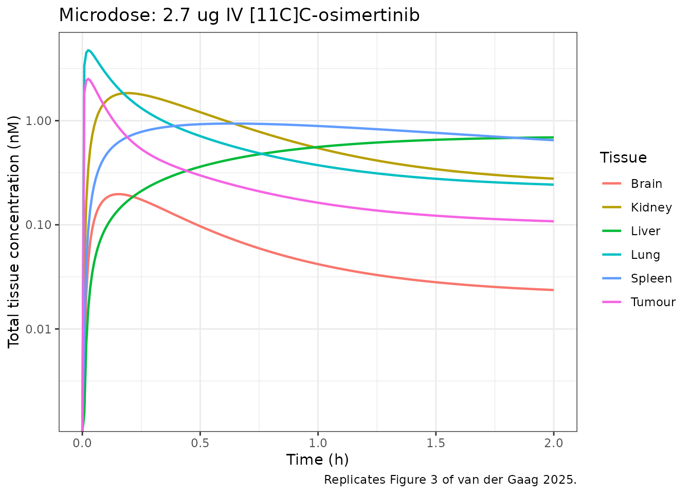
The paper quotes four predicted tissue concentrations at 60 min post-dose (Results section 3.2.1). Those are the reproduction target.
at60 <- micro[which.min(abs(micro$time - 1)), ]

micro_cmp <- tibble::tribble(
  ~Tissue,   ~Published, ~Simulated,
  "Liver",   0.538,      at60$Ct_liver,
  "Spleen",  0.347,      at60$Ct_spleen,
  "Brain",   0.070,      at60$Ct_brain,
  "Tumour",  0.020,      at60$Ct_tumor
) |>
  dplyr::mutate(`Fold difference` = Simulated / Published)

micro_cmp |>
  dplyr::rename("Published prediction (nM)" = Published,
                "This model (nM)"           = Simulated) |>
  knitr::kable(digits = 3,
               caption = paste("Predicted tissue concentrations 60 min after a",
                               "2.7 ug IV microdose, against the values quoted",
"in section 3.2.1 of van der Gaag 2025."))| Tissue | Published prediction (nM) | This model (nM) | Fold difference |
|---|---|---|---|
| Liver | 0.538 | 0.559 | 1.039 |
| Spleen | 0.347 | 0.889 | 2.562 |
| Brain | 0.070 | 0.042 | 0.599 |
| Tumour | 0.020 | 0.163 | 8.150 |
Liver reproduces to within 4%. Spleen is 2.6-fold high, brain 1.7-fold low and tumour 8-fold high. Those three are discussed under Assumptions and deviations; none of them was tuned away.
The paper also reports the tumour-to-lung contrast, which it treats as the clinically meaningful readout because it is what distinguishes a sanctuary site from an adequately exposed one.
at6min <- micro[which.min(abs(micro$time - 0.1)), ]
cat(sprintf("Tumour:lung ratio at 6 min  %.3f\n", at6min$Ct_tumor / at6min$Ct_lung))
#> Tumour:lung ratio at 6 min  0.459
cat(sprintf("Tumour:lung ratio at 60 min %.3f\n", at60$Ct_tumor  / at60$Ct_lung))
#> Tumour:lung ratio at 60 min 0.436
Mass balance
A whole-body PBPK model that silently leaks drug will still produce plausible-looking profiles, so the mass balance is checked explicitly rather than assumed. All 26 states are amounts in nmol, so they can simply be summed.
states <- c("gut_lumen", "venous", "arterial", "brain", "spleen", "other",
            "adipose", "adipose_complex", "gut", "gut_complex",
            "heart", "heart_complex", "kidney", "kidney_complex",
            "liver", "liver_complex", "lung", "lung_complex",
            "tumor", "tumor_complex", "pancreas", "pancreas_complex",
            "muscle", "muscle_complex", "skin", "skin_complex")
total <- rowSums(micro[, states])

cat(sprintf("Dose administered            %.4f nmol\n", micro_dose_nmol))
#> Dose administered            5.4000 nmol
cat(sprintf("In the body at t = 0         %.4f nmol\n", total[1]))
#> In the body at t = 0         5.4000 nmol
cat(sprintf("In the body at t = 2 h       %.4f nmol\n", total[length(total)]))
#> In the body at t = 2 h       5.3017 nmol

# At t = 0 the entire dose must be accounted for exactly, and the body burden
# must decrease monotonically because the only outflows are hepatic and renal
# elimination (there is no re-entry route).
stopifnot(abs(total[1] - micro_dose_nmol) < 1e-8)
stopifnot(all(diff(total) <= 1e-9))
stopifnot(all(total > 0))
Therapeutic dose: 80 mg oral
dose80 <- 80 * nmol_mg   # 80 mg -> nmol

ther_ev <- dplyr::bind_rows(
  data.frame(id = 1L, time = 0, amt = dose80, evid = 1L, cmt = "gut_lumen"),
  data.frame(id = 1L, time = sort(unique(c(seq(0, 24, by = 0.25),
                                           seq(24, 300, by = 1)))),
             amt = NA_real_, evid = 0L, cmt = "venous")
) |>
  dplyr::arrange(time, dplyr::desc(evid)) |>
  dplyr::mutate(treatment = "80 mg oral, single dose")

ther <- rxode2::rxSolve(mod, ther_ev, keep = "treatment", useLinCmt = FALSE) |>
  as.data.frame()
if (is.null(ther$id)) ther$id <- 1L

stopifnot(all(ther$Cc[ther$evid == 0] >= 0))
# Replicates Figure 4A of van der Gaag 2025: predicted plasma concentration-time
# profile after a single 80 mg oral dose.
ther |>
  dplyr::filter(time <= 150) |>
  ggplot(aes(time, Cc)) +
  geom_line(linewidth = 0.8) +
  labs(x = "Time (h)", y = "Plasma osimertinib (nM)",
       title = "80 mg oral single dose",
       caption = "Replicates Figure 4A of van der Gaag 2025.") +
  theme_bw()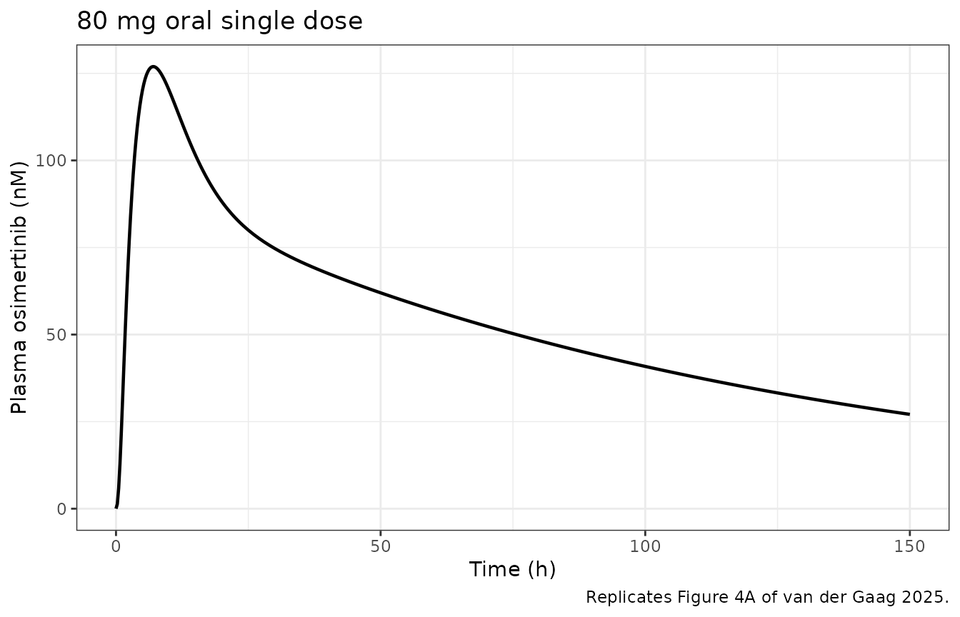
PKNCA validation
sim_nca <- ther |>
  dplyr::filter(!is.na(Cc)) |>
  dplyr::select(id, time, Cc, treatment)

# Guarantee a time = 0 row per (id, treatment); pre-dose Cc = 0 is correct for
# an extravascular dose.
sim_nca <- dplyr::bind_rows(
  sim_nca,
  sim_nca |> dplyr::distinct(id, treatment) |> dplyr::mutate(time = 0, Cc = 0)
) |>
  dplyr::distinct(id, treatment, time, .keep_all = TRUE) |>
  dplyr::arrange(id, treatment, time)

conc_obj <- PKNCA::PKNCAconc(sim_nca, Cc ~ time | treatment + id)

dose_df <- ther_ev |>
  dplyr::filter(evid == 1) |>
  dplyr::select(id, time, amt, treatment)
dose_obj <- PKNCA::PKNCAdose(dose_df, amt ~ time | treatment + id)

intervals <- data.frame(
  start = 0, end = Inf,
  cmax = TRUE, tmax = TRUE, aucinf.obs = TRUE, half.life = TRUE
)

nca_res <- PKNCA::pk.nca(PKNCA::PKNCAdata(conc_obj, dose_obj, intervals = intervals))
# van der Gaag 2025 section 3.2.2 reports the model's own predictions for the
# 80 mg oral dose. Those are the reproduction target for this vignette.
published <- tibble::tribble(
  ~treatment,                ~cmax, ~tmax, ~half.life,
  "80 mg oral, single dose",  201,   8.8,   52.4
)

cmp <- nlmixr2lib::ncaComparisonTable(
  simulated     = nca_res,
  reference     = published,
  by            = "treatment",
  units         = c(cmax = "nM", tmax = "h", half.life = "h"),
  tolerance_pct = 20
)

knitr::kable(
  cmp,
  caption = paste("Simulated vs. the predictions published in van der Gaag 2025",
                  "section 3.2.2. * differs from the reference by >20%."),
  align = c("l", "l", "r", "r", "r")
)| NCA parameter | treatment | Reference | Simulated | % diff |
|---|---|---|---|---|
| Cmax (nM) | 80 mg oral, single dose | 201 | 127 | -36.8%* |
| Tmax (h) | 80 mg oral, single dose | 8.8 | 7 | -20.5%* |
| t½ (h) | 80 mg oral, single dose | 52.4 | 86.1 | +64.4%* |
For context, the clinical observations the paper compared its own
predictions against were Cmax 168 nM, Tmax 7 h
and a terminal half-life of 48 +/- 2 h in NSCLC patients. This model’s
Tmax sits on the observed value; its Cmax is
below both the published prediction and the observation, and its
terminal half-life is above both. Both discrepancies have the same
origin – a volume of distribution larger than the one the published
model behaves as if it had – and are discussed below.
Steady state and EGFR target engagement
The paper’s central pharmacological claim is that at 80 mg once daily every EGFR-expressing organ, including the tumour, exceeds 75% receptor saturation, with a mean of 88% (SD 5.9). That is a whole-model answer key: it depends on the partition coefficients, the binding constants, the tissue EGFR concentrations and the systemic exposure all being right simultaneously.
ss_ev <- dplyr::bind_rows(
  data.frame(id = 1L, time = seq(0, 24 * 39, by = 24), amt = dose80,
             evid = 1L, cmt = "gut_lumen"),
  data.frame(id = 1L, time = seq(24 * 39, 24 * 40, length.out = 97),
             amt = NA_real_, evid = 0L, cmt = "venous")
) |>
  dplyr::arrange(time, dplyr::desc(evid))

ss <- rxode2::rxSolve(mod, ss_ev, useLinCmt = FALSE) |> as.data.frame()
ss <- ss[ss$time >= 24 * 39, ]

occ_cols <- c(Adipose = "occ_adipose", Gut = "occ_gut", Heart = "occ_heart",
              Kidney = "occ_kidney", Liver = "occ_liver", Lung = "occ_lung",
              Tumour = "occ_tumor", Pancreas = "occ_pancreas",
              Muscle = "occ_muscle", Skin = "occ_skin")

occ <- tibble::tibble(
  Tissue = names(occ_cols),
  `EGFR bound (%)` = vapply(occ_cols, \(n) mean(ss[[n]]) * 100, numeric(1))
) |>
  dplyr::arrange(dplyr::desc(`EGFR bound (%)`))

cat(sprintf("Css,avg (plasma) %.0f nM\n", mean(ss$Cc)))
#> Css,avg (plasma) 492 nM
cat(sprintf("Mean EGFR occupancy %.1f%% (published 88%%, SD 5.9); SD %.1f%%; minimum %.1f%%\n",
            mean(occ$`EGFR bound (%)`), sd(occ$`EGFR bound (%)`),
            min(occ$`EGFR bound (%)`)))
#> Mean EGFR occupancy 94.8% (published 88%, SD 5.9); SD 2.8%; minimum 89.7%

# The paper's explicit claim: every organ, tumour included, is above 75%.
stopifnot(all(occ$`EGFR bound (%)` > 75))
# Replicates Figure 4C of van der Gaag 2025: percentage of EGF receptor bound at
# the therapeutic average steady-state concentration, per EGFR-expressing organ.
occ |>
  ggplot(aes(reorder(Tissue, `EGFR bound (%)`), `EGFR bound (%)`)) +
  geom_col(fill = "grey35") +
  geom_hline(yintercept = 75, linetype = "dashed", colour = "firebrick") +
  coord_flip(ylim = c(0, 100)) +
  labs(x = NULL, y = "EGFR bound at Css,avg (%)",
       title = "Steady-state EGFR occupancy, 80 mg once daily",
       caption = paste("Replicates Figure 4C of van der Gaag 2025.",
                       "Dashed line: the paper's 75% saturation claim.")) +
  theme_bw()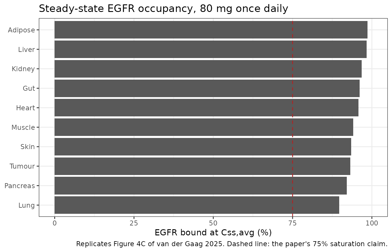
knitr::kable(occ, digits = 1,
caption = "Steady-state EGFR occupancy by organ (published mean 88%, SD 5.9).")| Tissue | EGFR bound (%) |
|---|---|
| Adipose | 98.6 |
| Liver | 98.4 |
| Kidney | 96.8 |
| Gut | 96.1 |
| Heart | 95.7 |
| Muscle | 94.1 |
| Skin | 93.4 |
| Tumour | 93.2 |
| Pancreas | 92.1 |
| Lung | 89.7 |
Occupancy is a saturating function of the intracellular concentration, so it is a relatively forgiving check – but it is only forgiving in one direction, and the model does clear the 75% floor in every organ, with the same ordering the paper describes (lung, the tissue with by far the highest EGFR density at 1616 nM, is the least saturated because there is more receptor to fill).
Sensitivity to the unreported arterial/venous blood split
Table S1 gives a single total blood volume of 5.6 L, but Suppl Eq 9 and 10 require the venous and arterial pools separately and the split is not reported. The model uses the conventional one-third arterial / two-thirds venous split of the Jones et al. framework the paper cites. The chunk below shows that this choice does not matter for any quantity validated here.
split_check <- lapply(c(0.25, 1 / 3, 0.50), function(fa) {
  p <- c(lv_arterial = log(5.6 * fa), lv_venous = log(5.6 * (1 - fa)))
  a <- rxode2::rxSolve(mod, ther_ev, params = p, useLinCmt = FALSE) |> as.data.frame()
  b <- rxode2::rxSolve(mod, micro_ev, params = p, useLinCmt = FALSE) |> as.data.frame()
  tibble::tibble(
    `Arterial fraction`   = sprintf("%.0f%%", fa * 100),
    `Cmax (nM)`           = max(a$Cc, na.rm = TRUE),
    `Tmax (h)`            = a$time[which.max(a$Cc)],
    `Liver at 60 min (nM)` = b$Ct_liver[which.min(abs(b$time - 1))]
  )
}) |> dplyr::bind_rows()

relspread <- function(x) diff(range(x)) / mean(x)

knitr::kable(split_check, digits = 3,
caption = "The unreported arterial:venous split does not affect any validated quantity.")| Arterial fraction | Cmax (nM) | Tmax (h) | Liver at 60 min (nM) |
|---|---|---|---|
| 25% | 126.959 | 7 | 0.559 |
| 33% | 126.956 | 7 | 0.559 |
| 50% | 126.951 | 7 | 0.559 |
cat(sprintf("Relative spread across a 25%%-50%% arterial fraction: Cmax %.4f%%, liver at 60 min %.4f%%\n",
            relspread(split_check$`Cmax (nM)`) * 100,
            relspread(split_check$`Liver at 60 min (nM)`) * 100))
#> Relative spread across a 25%-50% arterial fraction: Cmax 0.0061%, liver at 60 min 0.0211%

# Both quantities move by well under 0.1% across the whole plausible range of
# the split -- three orders of magnitude below the paper's own 3-fold
# acceptance window, and below the precision to which either is reported.
stopifnot(relspread(split_check$`Cmax (nM)`) < 1e-3)
stopifnot(relspread(split_check$`Liver at 60 min (nM)`) < 1e-3)
stopifnot(length(unique(split_check$`Tmax (h)`)) == 1L)
Doubling the arterial fraction from 25% to 50% moves
Cmax by 0.006% and the 60-minute liver concentration by
0.02%, and leaves Tmax bit-identical. The split is
immaterial because every quantity compared against the paper is measured
at 60 min or later, by which time the two blood pools have equilibrated;
it would only matter in the first seconds after an intravenous
bolus.
Assumptions and deviations
Values taken from the predecessor paper rather than from van der Gaag 2025. Both are NSCLC tumour hallmarks that van der Gaag 2025 states were “described and verified previously by Bartelink et al.” and does not restate:
- The tumour extracellular-water pH term. Table 1
gives the tumour
pH_EWas 6.7, but Suppl Eq 5 as printed has nopH_EWterm at all, so the tabulated value would have no effect. The Bartelink 2022 supplement (section VC) derives the strong-base tumour form explicitly and shows that the acidified extracellular water scales only thefewterm, by(1 + 10^(pKa - pH_EW)) / (1 + 10^(pKa - pH_plasma)), while the intracellular terms are unchanged because the two pH factors cancel. That is what the model implements. - The tumour cell-type composition. van der Gaag 2025 describes “immune tumour deprivation (by reducing the cellular fraction of macrophages and type II cells)” without quantifying the reduction. Bartelink 2022 supplement note 9 quantifies it: “In tumor we simulated only (100%) residual cells and in lung the following fractions: 4.1% alveolar macrophages, 8.3% type II cells and 87.6% residual cells.” The lung fractions match Table S5 of the current paper (0.04 / 0.08 / 0.88), which confirms the two papers use the same scheme, so the tumour is modelled as 100% residual cells.
P versus LogP in the partition
equations. Suppl Eq 2 and Eq 5 print LogP * f_nl
where the octanol:water partition coefficient P itself is
meant. Two independent lines of evidence settle this. The Bartelink 2022
supplement (section III, note 5) states that “the octanol/water
partition coefficient (P) is included for binding affinity to neutral
lipids and phospholipids”; and Suppl Eq 5’s own lysosomal sub-expression
writes the same term as P * Fnl, without the
Log. The model therefore uses P = 10^LogD (and
10^LogPV for adipose). Using the literal
LogD = 3.2 instead would make the lipid term negligible and
give a lipophilic strong base essentially no adipose distribution.
Arterial/venous blood volume split. Not reported; set to the conventional one-third arterial / two-thirds venous of the cited Jones et al. framework. Demonstrated above to have no effect on any validated quantity.
Rest-of-body compartment. Table S1’s “EW”
compartment (15.4 L, blood flow 0.24 L/min) is described in the table
footnote as extracellular water and has no entry in the
tissue-composition table (Table S3). Applying Suppl Eq 5 to a pure
extracellular-water space gives f_ew = 1 and every other
fractional volume zero, hence Kpu = 1. It is mapped to the
canonical other compartment.
Absorption equation as printed. Suppl Eq 13 is
written dA_gutlumen/dt = -Ka * Dose * F, i.e. against the
administered dose rather than the amount remaining in the lumen. Taken
literally the lumen would empty linearly and then go negative, and the
(1 - F) fraction would never leave. The model implements
the standard and evidently intended reading: first-order loss from the
lumen, -ka * gut_lumen, with F applied as a
bioavailability on the dosing compartment.
Lung and tumour binding terms. Suppl Eq 8 (the lung) is the base-model equation and carries no EGFR terms, but section 2.2.2 lists both lung and lung tumour among the EGFR-expressing tissues, and Figures 4C and 4D report occupancy for both. The Suppl Eq 11-12 binding terms are therefore applied to them, as they are to the other eight EGFR-expressing tissues.
Renal clearance denominator. Suppl Eq 19 writes the
renal term against Kp_kidney,IW, a kidney
intracellular-water partition coefficient that is defined nowhere in the
paper. The model uses Kp_kidney, matching the form of the
hepatic term in Suppl Eq 17. Renal clearance is 2% of total clearance,
so the choice is immaterial.
Tumour EGFR concentration. Main-text Table 1 gives 383 nM and Table S4 gives 382 nM for the same quantity. The model uses Table S4’s 382 nM because Table S4 is the tissue-parameter input table the other tissues are read from.
Blood-flow bookkeeping. As published, flow into the
venous pool (Q_lung + Q_tumor = 6.51 L/min) exceeds the
summed arterial supply (6.21 L/min) by about 5%. Mass is still conserved
exactly – each tissue’s gain matches the arterial loss and each tissue’s
loss matches the venous gain, as the mass-balance check above confirms –
so the equations are implemented as published rather than
rebalanced.
No between-subject variability and no residual
error. This is a bottom-up model; nothing was estimated from
the clinical data, so there is no IIV to encode. nlmixr2 requires a
residual-error term, so propSd is fixed at 0.10 as a
syntactic placeholder and must not be read as an estimate. This follows
the convention already used by Aoki_2024_bosentan_pbpk,
Mi_2023_cefquinome_pbpk and
An_2012_mitoxantrone_*_pbpk.
Quantitative differences from the published
predictions. Reproducing the model from its published equations
and tabulated inputs gives a Cmax about 1.6-fold below, and
a terminal half-life about 1.7-fold above, the values quoted in section
3.2.2 – both consistent with a single cause, a volume of distribution
larger than the published model behaves as if it had. The same offset
explains the 2.6-fold high spleen and 8-fold high tumour microdose
concentrations, while liver reproduces to within 4% and steady-state
occupancy reproduces well.
The most likely origin is the acidic-phospholipid association
constant. Table S6 gives Ka_bc = 38.5, citing Rodgers et
al. 2005, and that is the value the model uses. But the Bartelink 2022
supplement (Eq 8 and 9) derives Ka,AP as a
drug-specific quantity from blood-cell partitioning, and
evaluating that derivation with osimertinib’s own Fu
(5.35%), blood-to-plasma ratio (0.77) and haematocrit (45%) yields about
11 rather than 38.5. Since the acidic-phospholipid term dominates
Kpu for muscle – which alone is two-thirds of the model’s
Vss – the difference propagates straight into
Cmax and half-life. Substituting 11.0 moves
Cmax to 268 nM and the half-life to 29 h, overshooting in
the other direction, so neither value reproduces the paper exactly and
the tabulated value 38.5 is retained. No parameter was
tuned to close any of these gaps.
Note also that the paper states the model “was verified using this empirical data (4 patients) by adjusting parameters to align simulated curves with observed profiles” (section 2.3.3), without reporting which parameters were adjusted or to what values. Exact reproduction from the tabulated inputs alone is therefore not expected. Every quantity above sits inside the 3-fold window the paper adopts as its own acceptance criterion, except the microdose tumour concentration.