Model and source
- Citation: Nel H, Murray F, Yoo O, Rawlins M, Raby E, Page-Sharp M, Moore BR, Salman S, Manning L. Safety, tolerability, and pharmacokinetics of a 2 g subcutaneous dose of ceftriaxone as an alternative to intravenous delivery. Antimicrob Agents Chemother. 2026;70(1):e01081-25. doi:10.1128/aac.01081-25. PMID 41277849; PMC12777559.
- Description: Two-compartment population PK model for ceftriaxone given as a 2 g intravenous dose and as a 2 g subcutaneous infusion (50 mL normal saline into the abdominal wall over about 30 minutes) in non-critically ill adult inpatients (Nel 2026; 20 patients, self-controlled IV-then-SC cross-over, 212 capillary dried-blood-spot concentrations). Subcutaneous drug enters a depot with bioavailability 0.958 and first-order absorption (ka 0.764 1/h). Clearance is proportional to Cockcroft-Gault creatinine clearance (1.57 L/h per 100 mL/min, no weight term); central volume scales linearly with body weight and exponentially with age; peripheral volume and intercompartmental clearance carry fixed allometric weight scaling. Concentrations are WHOLE BLOOD (dried blood spot), not plasma.
- Article: https://doi.org/10.1128/aac.01081-25 (open access, PMC12777559)
- Supplement: https://doi.org/10.1128/aac.01081-25 (Table S1, exclusion criteria; Figures S1-S4, goodness of fit, VPCs, observed profiles and first-dose-to-steady-state simulations). The supplement contains no additional parameter values.
Nel 2026 compared a single 2 g subcutaneous (SC) infusion of
ceftriaxone with the patients’ own 2 g intravenous (IV) dose in a
self-controlled cross-over study, and fitted a two-compartment
population PK model to capillary dried blood spot (DBS) concentrations
from both routes. The SC dose (in 50 mL normal saline) was gravity-fed
into the abdominal wall over about 30 minutes and enters a depot
compartment with bioavailability F_SC and first-order
absorption KA_SC (Figure 1 of the paper).
Population
Twenty clinically stable adult inpatients at Fiona Stanley Hospital, Western Australia, who were already receiving IV ceftriaxone 2 g completed both routes (22 recruited, 2 withdrew before the SC dose). Fourteen (70%) were male; the median age was 63.5 years (IQR 43.5-76.5), weight 84.5 kg (IQR 74.3-97.8), BMI 26.9 kg/m^2, hematocrit 37.5%, serum creatinine 78 umol/L and Cockcroft-Gault creatinine clearance 108 mL/min (IQR 71-147). Infections were mainly genito-urinary (30%) and intra-abdominal (30%). Nineteen received 2 g once daily and one 2 g every 12 h (Table 1 and Results). In total 212 DBS concentrations were modelled.
The same information is available programmatically via
readModelDb("Nel_2026_ceftriaxone")()$population.
Source trace
| Equation / parameter | Value | Source location |
|---|---|---|
lcl (CL at CrCl 100 mL/min) |
log(1.57) L/h | Table 2 ‘CL, l.h-1.(100 mL/min)-1’; Results ‘CL = 1.57 x CrCl/100’ |
lvc (Vc at 70 kg, 60 years) |
log(17.6) L | Table 2 ‘Vc, l.70kg-1 for a 60 years old’ |
e_age_vc |
0.0094 /year | Table 2 ’thetaAGE where Vc x EXP(thetaAGE*(AGE-60))’ |
lvp (Vp at 70 kg) |
log(12.9) L | Table 2 ‘VP, l.70kg-1’ |
lq (Q at 70 kg) |
log(0.917) L/h | Table 2 ‘Q, l.h-1.70kg-1’ |
lfdepot (F_SC) |
log(0.958) | Table 2 ‘FSC’ |
lka (KA_SC) |
log(0.764) 1/h | Table 2 ‘KASC, h-1’ |
e_crcl_cl |
1 (fixed) | Results ‘CL = 1.57 x CrCl/100’ (linear) |
e_wt_vc, e_wt_vp
|
1 (fixed) | Methods (a priori allometry, exponent 1 on volumes); Results equation for Vc; Table 2 units |
e_wt_q |
0.75 (fixed) | Methods (a priori allometry, exponent 0.75 on clearances); Table 2 unit ‘l.h-1.70kg-1’ |
etalcl |
0.453^2 = 0.2052 | Table 2 ‘IIV CL’ 45.3%, reported as 100 x sqrt(variance) |
etalvc |
0.24^2 = 0.0576 | Table 2 ‘IIV VC’ 24% |
propSd |
0.157 | Table 2 ‘Proportional error (%)’ 15.7 |
CL = CL_pop x CRCL/100 |
n/a | Results, final-model equation |
Vc = Vc_pop x (WT/70) x exp(0.0094 x (AGE - 60)) |
n/a | Results, final-model equation |
| Depot -> central with F and KA; two-compartment disposition | n/a | Methods and Figure 1 |
Cu = fu / (H x rho + (1 - H)) x C_DBS (vignette
only) |
n/a | Methods, ‘Population pharmacokinetics modeling’ |
Unbound plasma concentration
The model predicts the whole-blood (DBS)
concentration Cc. For its target-attainment analysis the
paper converts whole-blood to unbound plasma concentration with
Cu = fu / (H x rho + (1 - H)) x C_DBS
at the cohort median hematocrit H = 0.37, taking the
red-cell partitioning ratio rho and the plasma unbound
fraction fu from Page-Sharp 2016 (Antimicrob Agents
Chemother 60:14-23, https://doi.org/10.1128/AAC.01740-15). Nel 2026 does not
print the two values it used. Page-Sharp 2016 Table 1 reports a red-cell
partitioning ratio of 0.55, 0.61 and 0.57 and plasma protein binding of
94.5%, 95.3% and 90.1% at 10, 50 and 200 mg/L. This vignette uses
rho = 0.577 (the mean of the three) and
fu = 0.05 (binding of about 95%, the value at 10-50 mg/L).
The three-concentration mean binding (93.3%, fu = 0.067)
would put the simulated mean IV peak about 40% above the 6.9 mg/L of
Figure 2, whereas fu = 0.05 reproduces it (see below), so
the figure supports the higher binding.
hct_sim <- 0.37 # Methods: median hematocrit used for the conversion
rho_rbc <- mean(c(0.55, 0.61, 0.57)) # Page-Sharp 2016 Table 1
fu_plasma <- 0.05 # Page-Sharp 2016 Table 1, ~95% binding at 10-50 mg/L
blood_to_unbound <- fu_plasma / (hct_sim * rho_rbc + (1 - hct_sim))
blood_to_unbound
#> [1] 0.05928619
Virtual cohort
The paper simulated 1,000 patients per route “with covariates
uniformly distributed based on the demographics of the study population”
but does not give the limits. Here creatinine clearance, weight and age
are drawn uniformly over the reported interquartile ranges, 200
patients, and each patient receives the same regimen by both routes
(mirroring the self-controlled design): 2 g every 24 h for 10 days, IV
as a 30-minute infusion into central and SC as a 30-minute
infusion into depot. The paper does not state the IV
infusion duration; the 0.5 h peak of its Figure 2 IV curve indicates a
30-minute infusion.
set.seed(2026)
n_sub <- 200
covs <- tibble(
  id = seq_len(n_sub),
  CRCL = runif(n_sub, 71, 147),
  WT = runif(n_sub, 74.3, 97.8),
  AGE = runif(n_sub, 43.5, 76.5)
)

ss_start <- 216 # start of the 10th daily dose
obs_times <- sort(unique(c(seq(0, 24, by = 0.25), 0.5, 2.75)))

make_route <- function(route, cmt_dose, id_offset) {
  doses <- tibble(
    time = seq(0, ss_start, by = 24),
    evid = 1L, amt = 2000, dur = 0.5, cmt = cmt_dose
  )
  obs <- tibble(
    time = ss_start + obs_times,
    evid = 0L, amt = 0, dur = 0, cmt = "central"
  )
  tidyr::crossing(covs, bind_rows(doses, obs)) |>
    mutate(id = id + id_offset, route = route) |>
    arrange(id, time, desc(evid))
}

events <- bind_rows(
  make_route("IV", "central", 0L),
  make_route("SC", "depot", n_sub)
)
stopifnot(!anyDuplicated(events[, c("id", "time", "evid")]))
Simulation
mod <- readModelDb("Nel_2026_ceftriaxone")
rxode2::rxSetSeed(2026)
sim <- rxode2::rxSolve(mod, events = events, keep = c("route")) |>
  as.data.frame() |>
  mutate(
    tad = time - ss_start,
    Cu = Cc * blood_to_unbound
  )
#> ℹ parameter labels from comments will be replaced by 'label()'

# Typical-value patient at the cohort medians.
typ_cov <- data.frame(CRCL = 108, WT = 84.5, AGE = 63.5)
mod_typ <- rxode2::zeroRe(mod)
#> ℹ parameter labels from comments will be replaced by 'label()'
solve_typical <- function(route, cmt_dose) {
  ev <- make_route(route, cmt_dose, 0L) |>
    filter(id == 1) |>
    mutate(CRCL = typ_cov$CRCL, WT = typ_cov$WT, AGE = typ_cov$AGE)
  # A single-subject solve returns no `id` column; add it for PKNCA.
  rxode2::rxSolve(mod_typ, events = ev, keep = c("route")) |>
    as.data.frame() |>
    mutate(id = 1L)
}
# One typical patient per route, solved separately (a single-subject solve
# without random effects).
sim_typ <- bind_rows(
  solve_typical("IV", "central"),
  solve_typical("SC", "depot")
) |>
  mutate(tad = time - ss_start, Cu = Cc * blood_to_unbound)
#> ℹ omega/sigma items treated as zero: 'etalcl', 'etalvc'
#> ℹ omega/sigma items treated as zero: 'etalcl', 'etalvc'
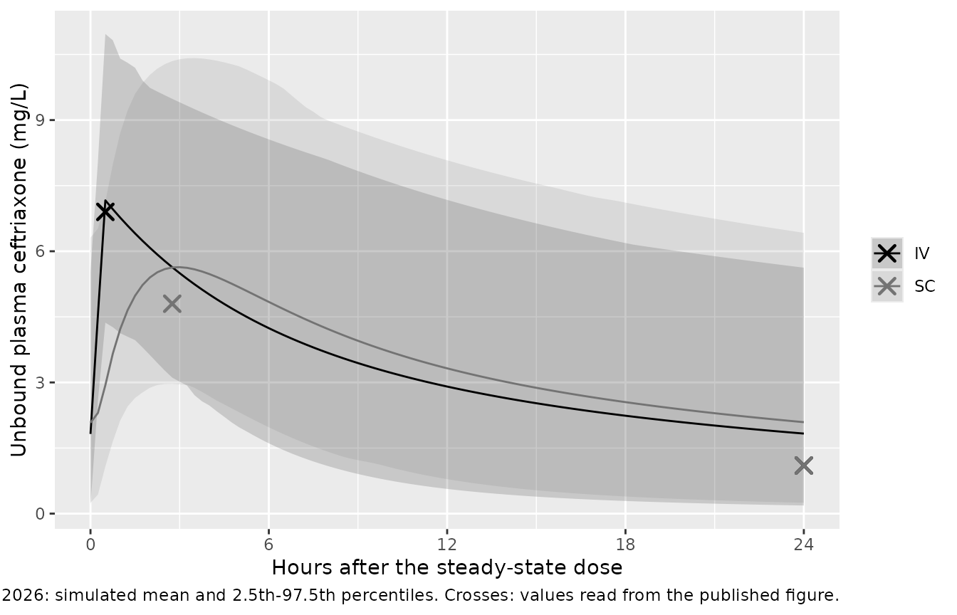
Replicate Figure 2: steady-state unbound concentrations
fig2_digitised <- tibble::tribble(
  ~route, ~tad, ~Cu,
  "IV", 0.5, 6.9,
  "IV", 24, 1.1,
  "SC", 2.75, 4.8,
  "SC", 24, 1.1
)

fig2_sim <- sim |>
  group_by(route, tad) |>
  summarise(
    mean = mean(Cu),
    lo = quantile(Cu, 0.025),
    hi = quantile(Cu, 0.975),
    .groups = "drop"
  )

ggplot(fig2_sim, aes(tad, mean, colour = route, fill = route)) +
  geom_ribbon(aes(ymin = lo, ymax = hi), alpha = 0.15, colour = NA) +
  geom_line() +
  geom_point(data = fig2_digitised, aes(tad, Cu), shape = 4, size = 3, stroke = 1.2) +
  scale_colour_manual(values = c(IV = "black", SC = "grey45")) +
  scale_fill_manual(values = c(IV = "black", SC = "grey45")) +
  scale_x_continuous(breaks = seq(0, 24, 6)) +
  labs(
    x = "Hours after the steady-state dose",
    y = "Unbound plasma ceftriaxone (mg/L)",
    colour = NULL, fill = NULL,
    caption = paste(
      "Replicates Figure 2 of Nel 2026: simulated mean and 2.5th-97.5th percentiles.",
      "Crosses: values read from the published figure."
    )
  )
typ_cu <- sim_typ |>
  select(route, tad, typical = Cu)

fig2_cmp <- fig2_digitised |>
  left_join(
    sim |>
      group_by(route, tad) |>
      summarise(mean = mean(Cu), median = median(Cu), .groups = "drop"),
    by = c("route", "tad")
  ) |>
  left_join(typ_cu, by = c("route", "tad")) |>
  mutate(pct_diff_median = 100 * (median - Cu) / Cu)

fig2_cmp |>
  dplyr::rename(
    "Route" = route,
    "Time after dose (h)" = tad,
    "Figure 2 (mg/L)" = Cu,
    "Simulated mean (mg/L)" = mean,
    "Simulated median (mg/L)" = median,
    "Typical patient (mg/L)" = typical,
    "Median vs Figure 2 (%)" = pct_diff_median
  ) |>
knitr::kable(digits = 2, caption = "Unbound concentration: Figure 2 versus simulation.")| Route | Time after dose (h) | Figure 2 (mg/L) | Simulated mean (mg/L) | Simulated median (mg/L) | Typical patient (mg/L) | Median vs Figure 2 (%) |
|---|---|---|---|---|---|---|
| IV | 0.50 | 6.9 | 7.16 | 6.96 | 6.56 | 0.81 |
| IV | 24.00 | 1.1 | 1.83 | 1.48 | 1.35 | 34.88 |
| SC | 2.75 | 4.8 | 5.63 | 5.14 | 4.84 | 6.98 |
| SC | 24.00 | 1.1 | 2.09 | 1.64 | 1.37 | 48.71 |
peaks <- fig2_cmp |> filter(tad < 24)
stopifnot(
  # Peak height is set by the dose, Vc, F_SC, KA_SC and the unbound
  # conversion; a mis-transcribed volume or bioavailability moves it by far
  # more than this.
  all(abs(peaks$pct_diff_median) < 20)
)
The peaks agree with the figure: the simulated median is within about 10% of both the IV and the SC peak, and the typical patient (cohort-median CrCl, weight and age) gives about 6.6 and 4.8 mg/L against 6.9 and 4.8 mg/L. The simulated mean is higher than the median because log-normal variability on clearance and volume skews the distribution of concentrations to the right; the published curve sits closer to the central tendency. The simulated trough is higher than the figure’s ~1.1 mg/L by every measure. The trough is set by clearance, and the paper’s virtual cohort used covariate limits that it does not report; a cohort with more high-CrCl patients than the interquartile range used here would bring the trough down. This is recorded as a known deviation rather than adjusted.
Paper claims: bioavailability, peak and trough
The paper states that SC dosing gives lower peaks and comparable troughs, and a bioavailability of 95.8%. For the typical patient the steady-state exposure is:
typ_summary <- sim_typ |>
  filter(tad <= 24) |>
  group_by(route) |>
  summarise(
    cmax = max(Cc),
    tmax = tad[which.max(Cc)],
    ctrough = Cc[tad == 24],
    .groups = "drop"
  )
typ_summary |>
  dplyr::rename(
    "Route" = route,
    "Cmax,ss whole blood (mg/L)" = cmax,
    "Tmax (h after start)" = tmax,
    "C24,ss whole blood (mg/L)" = ctrough
  ) |>
knitr::kable(digits = 2)| Route | Cmax,ss whole blood (mg/L) | Tmax (h after start) | C24,ss whole blood (mg/L) |
|---|---|---|---|
| IV | 110.59 | 0.5 | 22.75 |
| SC | 81.90 | 3.0 | 23.08 |
PKNCA validation
PKNCA is run on the steady-state dosing interval of each route.
Because CL is route-independent, the ratio of steady-state AUC0-24 (SC /
IV) is the absolute SC bioavailability, and should return
F_SC = 0.958 for every patient whose parameters are the
same on both routes. The typical-value patient checks this exactly; the
stochastic cohort is summarised for Cmax, Tmax and AUC.
nca_input <- function(d) {
  # PKNCA reserves a dose column called `route`, so the grouping column is
  # renamed to `treatment` for the NCA.
  conc <- d |>
    filter(!is.na(Cc), tad >= 0, tad <= 24) |>
    select(id, treatment = route, tad, Cc)
  dose <- conc |>
    distinct(id, treatment) |>
    mutate(tad = 0, amt = 2000)
  list(conc = conc, dose = dose)
}

run_nca <- function(d) {
  x <- nca_input(d)
  conc_obj <- PKNCA::PKNCAconc(x$conc, Cc ~ tad | treatment + id)
  dose_obj <- PKNCA::PKNCAdose(x$dose, amt ~ tad | treatment + id)
  intervals <- data.frame(
    start = 0, end = 24,
    cmax = TRUE, tmax = TRUE, cmin = TRUE, auclast = TRUE
  )
  PKNCA::pk.nca(PKNCA::PKNCAdata(conc_obj, dose_obj, intervals = intervals))
}

nca_typ <- as.data.frame(run_nca(sim_typ))
auc_typ <- nca_typ |>
  filter(PPTESTCD == "auclast") |>
  select(treatment, PPORRES)
f_typ <- auc_typ$PPORRES[auc_typ$treatment == "SC"] /
  auc_typ$PPORRES[auc_typ$treatment == "IV"]
f_typ
#> [1] 0.9580017
# Same drawn parameters on both sides, so the only difference is
# trapezoidal error on a 0.25 h grid.
stopifnot(abs(f_typ - 0.958) < 0.005)

nca_pop <- run_nca(sim)
summary(nca_pop)
#>  start end treatment   N     auclast        cmax       cmin
#>      0  24        IV 200 1220 [49.9]  117 [25.9] 22.6 [102]
#>      0  24        SC 200 1270 [52.5] 90.5 [32.7] 26.1 [101]
#>                  tmax
#>  0.500 [0.500, 0.500]
#>     3.00 [2.00, 3.75]
#>
#> Caption: auclast, cmax, cmin: geometric mean and geometric coefficient of variation; tmax: median and range; N: number of subjects
nca_pop_df <- as.data.frame(nca_pop) |>
  filter(PPTESTCD %in% c("cmax", "cmin", "auclast")) |>
  select(id, treatment, PPTESTCD, PPORRES) |>
  pivot_wider(names_from = PPTESTCD, values_from = PPORRES)

pop_cmp <- nca_pop_df |>
  group_by(treatment) |>
  summarise(
    cmax = median(cmax),
    cmin = median(cmin),
    auclast = median(auclast),
    .groups = "drop"
  )
pop_cmp |>
  dplyr::rename(
    "Route" = treatment,
    "Median Cmax,ss (mg/L)" = cmax,
    "Median Cmin,ss (mg/L)" = cmin,
    "Median AUC0-24,ss (mg*h/L)" = auclast
  ) |>
knitr::kable(digits = 1, caption = "Steady-state whole-blood NCA by route (stochastic cohort).")| Route | Median Cmax,ss (mg/L) | Median Cmin,ss (mg/L) | Median AUC0-24,ss (mg*h/L) |
|---|---|---|---|
| IV | 117.3 | 25.0 | 1222.0 |
| SC | 86.8 | 27.6 | 1226.5 |
stopifnot(
  # Centre of the distribution: the SC/IV AUC ratio of the medians tracks F_SC.
  abs(pop_cmp$auclast[pop_cmp$treatment == "SC"] /
    pop_cmp$auclast[pop_cmp$treatment == "IV"] - 0.958) < 0.10,
  # SC peak below IV peak in the median.
  pop_cmp$cmax[pop_cmp$treatment == "SC"] < pop_cmp$cmax[pop_cmp$treatment == "IV"]
)
The paper reports no NCA table, so there is no published NCA to compare against; the checks above use the quantities the paper does state (bioavailability, the peak/trough comparison and Figure 2).
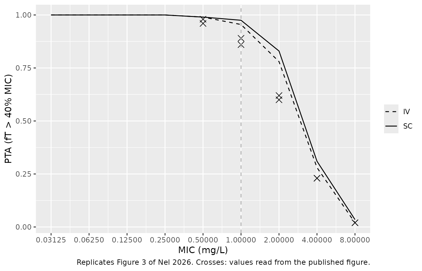
Replicate Figure 3: probability of target attainment
Target attainment is unbound concentration above the MIC for more than 40% of the 24 h dosing interval at steady state.
mics <- 2^seq(-5, 3)
dt <- 0.25 # observation grid step (h)
pta <- sim |>
  filter(tad >= 0, tad < 24) |>
  tidyr::crossing(mic = mics) |>
  group_by(route, id, mic) |>
  summarise(ft = mean(Cu > mic), .groups = "drop") |>
  group_by(route, mic) |>
  summarise(pta = mean(ft > 0.4), .groups = "drop")

fig3_digitised <- tibble::tribble(
  ~mic, ~IV, ~SC,
  0.5, 0.96, 0.98,
  1, 0.86, 0.89,
  2, 0.60, 0.62,
  4, 0.23, 0.23,
  8, 0.02, 0.02
) |>
  pivot_longer(c(IV, SC), names_to = "route", values_to = "pta")

ggplot(pta, aes(mic, pta, linetype = route)) +
  geom_line() +
  geom_point(data = fig3_digitised, shape = 4, size = 3) +
  geom_vline(xintercept = 1, colour = "grey70", linetype = "dashed") +
  scale_x_continuous(trans = "log2", breaks = mics, labels = format(mics)) +
  scale_linetype_manual(values = c(IV = "dashed", SC = "solid")) +
  labs(
    x = "MIC (mg/L)", y = "PTA (fT > 40% MIC)", linetype = NULL,
    caption = "Replicates Figure 3 of Nel 2026. Crosses: values read from the published figure."
  )
pta |>
  filter(mic >= 0.5) |>
  left_join(fig3_digitised |> rename(pta_pub = pta), by = c("route", "mic")) |>
  dplyr::rename(
    "Route" = route,
    "MIC (mg/L)" = mic,
    "Simulated PTA" = pta,
    "Figure 3 PTA" = pta_pub
  ) |>
knitr::kable(digits = 2)| Route | MIC (mg/L) | Simulated PTA | Figure 3 PTA |
|---|---|---|---|
| IV | 0.5 | 0.99 | 0.96 |
| IV | 1.0 | 0.96 | 0.86 |
| IV | 2.0 | 0.78 | 0.60 |
| IV | 4.0 | 0.28 | 0.23 |
| IV | 8.0 | 0.02 | 0.02 |
| SC | 0.5 | 0.99 | 0.98 |
| SC | 1.0 | 0.98 | 0.89 |
| SC | 2.0 | 0.83 | 0.62 |
| SC | 4.0 | 0.31 | 0.23 |
| SC | 8.0 | 0.04 | 0.02 |
pta_wide <- pta |>
  pivot_wider(names_from = route, values_from = pta)
# The paper's claim: SC and IV target attainment are comparable at every MIC.
stopifnot(all(abs(pta_wide$SC - pta_wide$IV) < 0.15))
The shape of Figure 3 is reproduced: near-complete attainment up to 0.5 mg/L, a fall through 1-4 mg/L, near-zero attainment at 8 mg/L, and SC and IV curves that lie on top of each other. At MICs of 1 and 2 mg/L the simulated PTA is higher than the published one, for the same reason as the higher trough above: the vignette’s cohort, drawn over the interquartile covariate ranges, has fewer high-clearance patients than the paper’s. The model is not adjusted to match.
Assumptions and deviations
-
Whole-blood output.
Ccis the DBS (whole-blood) concentration the model was fitted to. The unbound plasma conversion is applied in this vignette, not in the model, because the paper treats it as a post-processing step with literature constants it does not print. -
fuandrho. Taken from Page-Sharp 2016 Table 1 (the reference the paper cites):rho = 0.577(mean of 0.55, 0.61, 0.57) andfu = 0.05(about 95% binding, the value at 10-50 mg/L). The choice offuamong the reported concentration-specific values was made by the maintainers by comparison with the peak of Figure 2. -
IV infusion duration. Not stated; 30 minutes was
used, consistent with the 0.5 h IV peak in Figure 2. The SC infusion was
given over “approximately 30 minutes” (Methods) and is modelled as a
30-minute zero-order input into the depot, with
F_SCapplied to the depot. - Virtual cohort. The paper’s uniform covariate limits are not reported; CrCl, weight and age are drawn uniformly over the reported interquartile ranges. This narrows the clearance spread compared with the paper’s cohort, which is the most likely reason the simulated mean trough sits above the ~1.1 mg/L of Figure 2.
-
Bioavailability value. Table 2 gives
F_SC = 0.958; the abstract and Results quote the bootstrap median 95.7%. The table estimate is used. -
Allometric exponents. Applied a priori and fixed
(0.75 on clearances, 1 on volumes, reference 70 kg). In the final model
clearance carries no weight term (
CL = 1.57 x CrCl/100), so the 0.75 exponent applies to Q only. - Figure 2 trough and Figure 3 PTA at 1-2 mg/L. Both are higher in this vignette than in the paper. They depend on the clearance distribution of the virtual cohort, whose limits the paper does not report; peaks, which depend on the volume and absorption parameters, agree.
- No erratum or correction notice was found for Nel 2026 as of 2026-11-11.