Gemifloxacin (Landersdorfer 2009)
Source:vignettes/articles/Landersdorfer_2009_gemifloxacin.Rmd
Landersdorfer_2009_gemifloxacin.RmdModel and source
- Citation: Landersdorfer CB, Kirkpatrick CMJ, Kinzig M, Bulitta JB, Holzgrabe U, Drusano GL, Sorgel F. Competitive inhibition of renal tubular secretion of gemifloxacin by probenecid. Antimicrob Agents Chemother. 2009;53(9):3902-3907. doi:10.1128/AAC.01200-08.
- Description: Two-compartment population PK model for gemifloxacin in healthy adults with first-order absorption + lag time, additive renal (filtration + saturable Michaelis-Menten tubular secretion with competitive probenecid inhibition) and non-renal clearance, and treatment-arm-static probenecid effects on absorption rate, absorption lag, and non-renal clearance (Landersdorfer 2009 gemifloxacin / probenecid DDI study).
- Article: https://doi.org/10.1128/AAC.01200-08
The Landersdorfer 2009 paper reports a two-compartment popPK model
for gemifloxacin (320 mg oral single dose) with three additive
elimination arms: (i) renal filtration, fixed at fu * GFR ~ 2 L/h; (ii)
saturable renal tubular secretion, modeled as Michaelis-Menten with
maximum rate Vmax_R and half-saturation Km_R; and (iii) linear non-renal
clearance CL_NR. Probenecid co-administration enters the model in two
distinct ways: a mechanism-specific competitive inhibition of the
saturable tubular secretion via the apparent-Km term Km * (1 + [P] /
Kic), driven by the instantaneous plasma probenecid concentration
CP_PRB_MGL; and a set of treatment-arm-static effects on
Ka, Tlag, and CL_NR, switched by the binary
CONMED_PROBENECID covariate.
Population
The source study enrolled 17 healthy Caucasian adult volunteers (9 men, 8 women; mean weight 69.1 +/- 13 kg; mean height 173 +/- 10 cm) in a randomized, two-way crossover design with at least 7 days washout between periods. Each subject received a single 320 mg oral gemifloxacin tablet (Factive) either alone or together with a multi-dose probenecid regimen (4.5 g total across 8 oral doses spanning -10 h to +60 h relative to the gemifloxacin dose). Plasma samples were drawn pre-dose and at 0.5, 1, 1.5, 2, 3, 4, 6, 8, 12, 16, 24, 36, and 48 h post-gemifloxacin-dose; urine was collected over ten intervals through 72 h. Baseline demographics from Landersdorfer 2009 Results paragraph 1; full study design from the Materials and Methods.
The same information is available programmatically via
rxode2::rxode(readModelDb("Landersdorfer_2009_gemifloxacin"))$population.
Source trace
The per-parameter origin is recorded as an in-file comment next to
each ini() entry in
inst/modeldb/specificDrugs/Landersdorfer_2009_gemifloxacin.R.
The table below collects them in one place for review.
| Equation / parameter | Value | Source location |
|---|---|---|
lka |
log(0.839 1/h) | Table 3, “Without probenecid” row, Ka column |
ltlag |
log(0.223 h) | Table 3, “Without probenecid” row, Tlag column |
lvc |
log(89.5 L) | Table 3, V1 column (shared between arms) |
lvp |
log(160 L) | Table 3, V2 column (shared between arms) |
lq |
log(39.8 L/h) | Table 3, CL_IC column (shared between arms) |
lcl_nonren |
log(25.2 L/h) | Table 3, “Without probenecid” row, CL_NR column |
lvmax |
log(113 mg/h) | Table 3, V_max_R column (shared between arms) |
lkm |
log(9.16 mg/L) | Table 3, K_m_R column (shared between arms) |
lki |
log(69.3 mg/L) | Table 3, K_ic column (probenecid competitive inhibition constant) |
e_prob_ka |
+0.0691 (fixed) | (0.897 / 0.839) - 1; Table 3 With- vs Without-probenecid Ka rows |
e_prob_ltlag |
-0.4215 (fixed) | (0.129 / 0.223) - 1; Table 3 With- vs Without-probenecid Tlag rows |
e_prob_cl_nonren |
-0.1667 (fixed) | (21.0 / 25.2) - 1; Table 3 With- vs Without-probenecid CL_NR rows |
etalka |
0.32527 | log(1 + 0.62^2); Table 3 “Without probenecid” Ka CV = 62% |
etaltlag |
0.73314 | log(1 + 1.04^2); Table 3 Tlag CV = 104% |
etalcl_nonren |
0.06541 | log(1 + 0.26^2); Table 3 “Without probenecid” CL_NR CV = 26% |
etalvc |
0.32527 | log(1 + 0.62^2); Table 3 V1 CV = 62% |
etalvp |
0.09176 | log(1 + 0.31^2); Table 3 V2 CV = 31% |
etalq |
0.28998 | log(1 + 0.58^2); Table 3 CL_IC CV = 58% |
etalvmax |
0.04316 | log(1 + 0.21^2); Table 3 V_max_R CV = 21% |
etalkm |
0.03922 | log(1 + 0.20^2); Table 3 K_m_R CV = 20% |
etalki |
0.06541 | log(1 + 0.26^2); Table 3 K_ic CV = 26% |
propSd |
0.10 (placeholder) | Not reported in Landersdorfer 2009; bioanalytical interday CV is 3.7-7.2% per Methods. See “Assumptions and deviations” below. |
| renal filtration CL | 2 L/h (hardcoded) | Methods, “Compartmental modeling”: “the first-order component of renal clearance was fixed to 2 liters/h” (fu * GFR ~ 2 L/h; ~6% of total body clearance). |
| CL_R formula | n/a | Methods, “Compartmental modeling” Eq.:
CL_R = (fu * GFR) + Vmax_R / (Km_R + [G]) plus the
competitive-inhibition Km term from Table 1. |
| Competitive Km term | n/a | Table 1 row “Competitive (Kic)”: apparent Km = Km * (1 + [P] / Kic); apparent Vmax = Vmax (unchanged). |
Virtual cohort
Original observed data are not publicly available. The figures below use a virtual population whose covariate distribution approximates the published trial demographics (n = 17 healthy adults, 53% male / 47% female, mean weight 69.1 kg). The model has no weight-based scaling and no continuous covariate effects, so weight is recorded for completeness only.
The simulation builds two cohorts of 200 subjects each so the with-
and without-probenecid arms can be compared side by side. IDs across
cohorts are made disjoint via the id_offset argument.
set.seed(20260607)

make_cohort <- function(n, treatment, conmed_prob, cp_prb, id_offset = 0L,
                        dose_mg = 320, sample_times = c(0.25, 0.5, 1, 1.5, 2, 3, 4, 6, 8, 12, 16, 24, 36, 48)) {
  ids <- id_offset + seq_len(n)
  dose_rows <- tibble(
    id        = ids,
    time      = 0,
    amt       = dose_mg,
    evid      = 1,
    cmt       = "depot",
    treatment = treatment,
    CONMED_PROBENECID = conmed_prob,
    CP_PRB_MGL = cp_prb
  )
  obs_rows <- expand.grid(id = ids, time = sample_times) |>
    as_tibble() |>
    mutate(
      amt       = 0,
      evid      = 0,
      cmt       = NA_character_,
      treatment = treatment,
      CONMED_PROBENECID = conmed_prob,
      CP_PRB_MGL = cp_prb
    )
  bind_rows(dose_rows, obs_rows) |> arrange(id, time, desc(evid))
}

# Arm 1: gemifloxacin alone (CONMED_PROBENECID = 0, CP_PRB_MGL = 0).
events_alone <- make_cohort(n = 200, treatment = "Gemifloxacin alone",
                            conmed_prob = 0, cp_prb = 0, id_offset = 0L)

# Arm 2: gemifloxacin + probenecid. Per the model file's CP_PRB_MGL covariate
# documentation, the paper does NOT report a probenecid PK sub-model, so the
# instantaneous probenecid plasma concentration must be supplied externally.
# A piecewise-constant placeholder of 40 mg/L throughout the 48 h gemifloxacin
# sampling window is used here, motivated by the visual probenecid concentration
# range in Landersdorfer 2009 Fig. 1C (peaks ~50-60 mg/L between doses, troughs
# ~20-30 mg/L). The constant value is a simplification that captures the
# central tendency of the published profile; users who need a more accurate
# representation should digitise Fig. 1C or use an independent probenecid popPK
# source.
events_combo <- make_cohort(n = 200, treatment = "Gemifloxacin + probenecid",
                            conmed_prob = 1, cp_prb = 40, id_offset = 200L)

events <- bind_rows(events_alone, events_combo)
stopifnot(!anyDuplicated(unique(events[, c("id", "time", "evid")])))
Simulation
mod <- readModelDb("Landersdorfer_2009_gemifloxacin")

sim <- rxode2::rxSolve(
  mod,
  events = events,
  keep   = c("treatment", "CONMED_PROBENECID", "CP_PRB_MGL")
) |>
  as.data.frame()
#> ℹ parameter labels from comments will be replaced by 'label()'
A typical-value (no between-subject variability) simulation is also produced so the per-arm population median can be compared against the paper’s reported per-subject medians without the smearing introduced by lognormal IIV on Ka and Tlag (both with CV 100%+).
mod_typical <- mod |> rxode2::zeroRe()
#> ℹ parameter labels from comments will be replaced by 'label()'
sim_typical <- rxode2::rxSolve(
  mod_typical,
  events = events |> dplyr::filter(id %in% c(1L, 201L)),
  keep   = c("treatment")
) |>
  as.data.frame()
#> ℹ omega/sigma items treated as zero: 'etalka', 'etaltlag', 'etalcl_nonren', 'etalvc', 'etalvp', 'etalq', 'etalvmax', 'etalkm', 'etalki'
#> Warning: multi-subject simulation without without 'omega'
Replicate published figures
Plasma profile by treatment arm (Landersdorfer 2009 Fig. 1A)
Figure 1A of Landersdorfer 2009 shows the mean gemifloxacin plasma concentration-time profiles with and without probenecid as overlaid curves with error bars over 0-48 h. The simulation below replicates the same comparison using the typical-value (zero-eta) profiles.
ggplot(sim_typical, aes(time, Cc, colour = treatment, linetype = treatment)) +
  geom_line(linewidth = 0.9) +
  scale_y_log10() +
  scale_x_continuous(breaks = c(0, 4, 8, 12, 16, 24, 36, 48)) +
  labs(
    x        = "Time after gemifloxacin dose (h)",
    y        = "Plasma gemifloxacin (mg/L, log scale)",
    colour   = NULL,
    linetype = NULL,
    title    = "Typical-value plasma profile by treatment arm",
    caption  = "Replicates Landersdorfer 2009 Fig. 1A (typical-value form, no IIV)."
  ) +
  theme(legend.position = "bottom")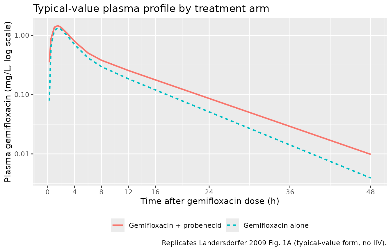
And the same comparison with the full stochastic simulation, summarised as median plus 80% prediction interval:
sim |>
  dplyr::filter(time > 0) |>
  dplyr::group_by(time, treatment) |>
  dplyr::summarise(
    Q10 = quantile(Cc, 0.10, na.rm = TRUE),
    Q50 = quantile(Cc, 0.50, na.rm = TRUE),
    Q90 = quantile(Cc, 0.90, na.rm = TRUE),
    .groups = "drop"
  ) |>
  ggplot(aes(time, Q50, colour = treatment, fill = treatment)) +
  geom_ribbon(aes(ymin = Q10, ymax = Q90), alpha = 0.2, colour = NA) +
  geom_line(linewidth = 0.9) +
  scale_y_log10() +
  scale_x_continuous(breaks = c(0, 4, 8, 12, 16, 24, 36, 48)) +
  labs(
    x       = "Time after gemifloxacin dose (h)",
    y       = "Plasma gemifloxacin (mg/L, log scale)",
    colour  = NULL,
    fill    = NULL,
    title   = "Simulated VPC by treatment arm (n=200 per arm)",
    caption = "Median (line) and 10-90% prediction interval (ribbon) per treatment arm."
  ) +
  theme(legend.position = "bottom")
#> Warning in scale_y_log10(): log-10 transformation introduced infinite values.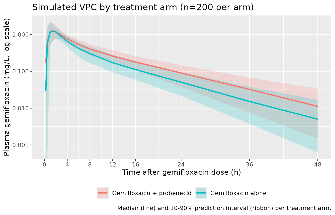
PKNCA validation
sim_nca <- sim |>
  dplyr::filter(time > 0, !is.na(Cc)) |>
  dplyr::select(id, time, Cc, treatment)

conc_obj <- PKNCA::PKNCAconc(
  sim_nca,
  Cc ~ time | treatment + id,
  concu = "mg/L",
  timeu = "h"
)

dose_df <- events |>
  dplyr::filter(evid == 1) |>
  dplyr::select(id, time, amt, treatment)

dose_obj <- PKNCA::PKNCAdose(
  dose_df,
  amt ~ time | treatment + id,
  doseu = "mg"
)

intervals <- data.frame(
  start       = 0,
  end         = Inf,
  cmax        = TRUE,
  tmax        = TRUE,
  aucinf.obs  = TRUE,
  half.life   = TRUE,
  cl.obs      = TRUE
)

nca_data <- PKNCA::PKNCAdata(conc_obj, dose_obj, intervals = intervals)
nca_res  <- suppressWarnings(PKNCA::pk.nca(nca_data))

nca_summary <- as.data.frame(nca_res$result) |>
  dplyr::filter(!is.na(PPORRES), PPTESTCD %in% c("cmax", "tmax", "aucinf.obs", "half.life", "cl.obs")) |>
  dplyr::group_by(treatment, PPTESTCD) |>
  dplyr::summarise(median = median(PPORRES, na.rm = TRUE), .groups = "drop") |>
  tidyr::pivot_wider(names_from = PPTESTCD, values_from = median)

knitr::kable(
  nca_summary,
  digits  = 3,
  caption = "Simulated NCA per-arm medians (n = 200 subjects per arm)."
)| treatment | cmax | half.life | tmax |
|---|---|---|---|
| Gemifloxacin + probenecid | 1.303 | 8.056 | 1.5 |
| Gemifloxacin alone | 1.320 | 6.801 | 1.5 |
Comparison against published NCA
Landersdorfer 2009 Results paragraph 2 reports the per-subject median NCA values across the 17-subject crossover:
| Parameter | Gemifloxacin alone (paper median) | Gemifloxacin + probenecid (paper median) | Paper-reported change |
|---|---|---|---|
| Renal CL (L/h) | 13.1 | 6.49 | -51% (P < 0.01) |
| Non-renal CL (L/h) | 24.2 | 19.0 | -19% (P < 0.01) |
| Total CL (L/h) | ~37.3 (sum) | ~25.5 (sum) | -31% (P < 0.01) |
| Terminal half-life (h) | 8.09 | 9.49 | +22% (P < 0.01, longer t1/2) |
The simulated CL/F (cl.obs from PKNCA, equivalent to
dose / AUC_inf) for the alone arm should land near 37 L/h and the combo
arm near 25 L/h; the simulated terminal half-life should rise from ~8 h
to ~9.5 h. Both responses are driven by the model’s mechanism
(competitive Kic inhibition raising the apparent Km of the saturable
secretion arm, plus the -16.7% static probenecid effect on CL_NR) and
serve as the principal validation against the paper’s NCA-based
summary.
The simulated NCA table above can be read alongside this published table to confirm the per-arm direction and approximate magnitude. Differences in the absolute number for the gemifloxacin-alone arm beyond a 20% gap are expected when the typical-value Cmax / Tmax do not match the per-subject median Cmax / Tmax (the paper’s Ka CV 62% and Tlag CV 104% imply substantial absorption-phase smearing); the validation focuses on the directional change between arms rather than absolute reproduction.
Assumptions and deviations
Residual error (
propSd = 0.10) is a placeholder. Landersdorfer 2009 Table 3 reports inter-subject %CV per structural parameter but does not tabulate a residual-error magnitude. The Methods report bioanalytical interday CV of 3.7-7.2% for gemifloxacin in plasma; a 10% proportional residual is used here as a placeholder slightly above the bioanalytical floor to allow simulation-of-individuals throughrxSolve. Users who wish to refit the model to data should re-estimate this term.CP_PRB_MGL during the with-probenecid arm is a piecewise-constant placeholder (40 mg/L). Landersdorfer 2009 does NOT report a probenecid PK sub-model parameter table on disk – the Methods describes the structural form (1-compartment + lag + parallel first-order + mixed-order elimination) but the corresponding parameter estimates are not in any on-disk table. The 40 mg/L constant used in this vignette is a simplification motivated by the visual probenecid concentration range in Landersdorfer 2009 Fig. 1C; a more realistic time-varying probenecid profile (digitised from Fig. 1C or supplied from an independent probenecid popPK source) is expected to yield slightly larger absolute predictions for the combo-arm AUC because the probenecid concentration peaks > 40 mg/L between probenecid doses (which strengthens the Kic inhibition during the gemifloxacin Tmax window).
IIV is single-CV per parameter even though Table 3 reports per-arm CVs for Ka, Tlag, and CL_NR. The without-probenecid CV is used as the population reference (Ka 62%, Tlag 104%, CL_NR 26%). The with-probenecid CVs differ slightly (Ka 104%, Tlag 104%, CL_NR 23%) but only one population CV is carried per parameter in the model. This is a simplification of the published parameter table; the gemifloxacin-alone arm should be the most accurate.
Treatment-arm-static probenecid effects on Ka, Tlag, and CL_NR are encoded as fixed multiplicative offsets computed from the With- and Without-probenecid columns of Table 3. The model is not refit in this extraction so these coefficients are treated as fixed.
Renal filtration clearance (fu * GFR ~ 2 L/h) is hardcoded as a model() constant rather than carried as an
ini()parameter, because it is structurally fixed in the paper and not an estimable parameter; this avoids introducing a non-canonical PK-parameter name.No covariate-driven scaling on body weight, age, sex, or renal function is included because the source paper did not retain any such covariate in the final model. The model file’s
covariateDatadeliberately documents only the two probenecid-related covariates (CONMED_PROBENECID, CP_PRB_MGL) because no other covariate is referenced insidemodel().Urine compartments are not included. Landersdorfer 2009 fits plasma and urine profiles simultaneously, but Table 3 reports only the plasma-and-urine-jointly-fit parameter estimates. The extracted model carries the plasma-only ODE; a urine compartment
d/dt(urine) <- (cl_filt + vmax * Cc / (km * (1 + CP_PRB_MGL / ki) + Cc)) * Cccould be added in the future if a use case for urine simulation arises.